Spontaneous rotational symmetry breaking and roton like excitations in gauged $\sigma$-model at finite density

Abstract

The linear $\sigma$-model with a chemical potential for hypercharge is a toy model for the description of the dynamics of the kaon condensate in high density QCD. We analyze the dynamics of the gauged version of this model. It is shown that spontaneous breakdown of $SU(2)\times U(1)_{Y}$ symmetry, caused by the chemical potential, is always accompanied by spontaneous breakdown of both rotational symmetry and electromagnetic $U(1)_{em}$. The spectrum of excitations in this model is rich and, because of rotational symmetry breakdown, anisotropic. It is shown that there exist excitation branches that behave as phonon like quasiparticles for small momenta and as roton like ones for large momenta. This suggests that this model can be relevant for anisotropic superfluid systems.

I Introduction

Recently a class of relativistic models with a finite density of matter has been revealed in which spontaneous breakdown of continuous symmetries leads to a lesser number of Nambu-Goldstone (NG) bosons than that required by the Goldstone theorem MS ; STV . It is noticeable that this class, in particular, describes the dynamics of the kaon condensate in the color-flavor locked phase of high density QCD that may exist in cores of compact stars BS .

The simplest representative of this class is the linear $SU(2)_{L}\times SU(2)_{R}$ $\sigma$-model with the chemical potential for the hypercharge $Y$:

$${\cal L}=(\partial_{0}+i\mu)\Phi^{\dagger}(\partial_{0}-i\mu)\Phi-\partial_{i}\Phi^{\dagger}\partial_{i}\Phi-m^{2}\Phi^{\dagger}\Phi-\lambda(\Phi^{\dagger}\Phi)^{2},$$ (1)

where $\Phi$ is a complex doublet field. The chemical potential $\mu$ is provided by external conditions (to be specific, we take $\mu>0$). For example, in the case of dense QCD with the kaon condensate, $\mu=m^{2}_{s}/2p_{F}$ where $m_{s}$ is the current mass of the strange quark and $p_{F}$ is the quark Fermi momentum BS . Note that the terms with the chemical potential reduce the initial $SU(2)_{L}\times SU(2)_{R}$ symmetry to the $SU(2)_{L}\times U(1)_{Y}$ one. This follows from the fact that the hypercharge generator $Y$ is $Y=2I^{3}_{R}$ where $I^{3}_{R}$ is the third component of the right handed isospin generator. Henceforth we will omit the subscripts $L$ and $R$, allowing various interpretations of the $SU(2)$ [for example, in the dynamics of the kaon condensate, it is just the conventional isospin symmetry $SU(2)_{I}$ and $\Phi^{T}=(K^{+},K^{0}$)].

The terms containing the chemical potential in Eq. (1) are

$$i\mu\Phi^{\dagger}\partial_{0}\Phi-i\mu\partial_{0}\Phi^{\dagger}\Phi+\mu^{2}\Phi^{\dagger}\Phi.$$ (2)

The last term in this expression makes the mass term in Lagrangian density (1) to be $(\mu^{2}-m^{2})\Phi^{\dagger}\Phi$. Therefore for supercritical values of the chemical potential, $\mu^{2}>m^{2}$, there is an instability resulting in the spontaneous breakdown of $SU(2)\times U(1)_{Y}$ down to $U(1)_{em}$ connected with the electrical charge $Q_{em}=I^{3}+\frac{1}{2}Y$. One may expect that this implies the existence of three NG bosons. However, as was shown in Refs. MS ; STV , there are only two NG bosons, which carry the quantum numbers of $K^{+}$ and $K^{0}$ mesons. The third would-be NG boson, with the quantum numbers of $K^{-}$, is massive in this model. This happens despite the fact that the potential part of Lagrangian (1) has three flat directions in the broken phase, as it should. The splitting between $K^{+}$ and $K^{-}$ occurs because of the seesaw mechanism in the kinetic part of the Lagrangian density (kinetic seesaw mechanism) MS . This mechanism is provided by the first two terms in expression (2) which, because of the imaginary unit in front, mix the real and imaginary parts of the field $\Phi$. Of course this effect is possible only because the $C$, $CP$, and $CPT$ symmetries are explicitly broken in this system at a nonzero $\mu$.

Another noticeable point is that while the dispersion relation for $K^{0}$ is conventional, with the energy $\omega\sim k$ as the momentum $k$ goes to zero, the dispersion relation for $K^{+}$ is $\omega\sim k^{2}$ for small $k$ MS ; STV . This fact is in accordance with the Nielsen-Chadha counting rule, $N_{G/H}=n_{1}+2n_{2}$ NC . Here $n_{1}$ is the number of NG bosons with the linear dispersion law, $\omega\sim k$, $n_{2}$ is the number of NG bosons with the quadratic dispersion law $\omega\sim k^{2}$, and $N_{G/H}$ is the number of the generators in the coset space $G/H$ (here $G$ is the symmetry group of the action and $H$ is the symmetry group of the ground state).

Does the conventional Anderson-Higgs mechanism survive in the gauged version of this model despite the absence of one out of three NG bosons? This question has motivated the present work.

II Gauged $\sigma$-model

We will consider the dynamics in the gauged version of model (1), i.e., the model described by the Lagrangian density

$${\cal L}=-\frac{1}{4}F_{\mu\nu}^{(a)}F^{\mu\nu(a)}-\frac{1}{4}B_{\mu\nu}B^{\mu\nu}+[(D_{\mu}-i\mu\delta_{\mu 0})\Phi]^{\dagger}(D^{\mu}-i\mu\delta^{\mu 0})\Phi-m^{2}\Phi^{\dagger}\Phi-\lambda(\Phi^{\dagger}\Phi)^{2},$$ (3)

where the covariant derivative $D^{\mu}=\partial_{\mu}-igA_{\mu}-(ig^{\prime}/2)B_{\mu}$, and

$$\Phi=\left(\begin{array}[]{c}0\\ \varphi_{0}\end{array}\right)+\frac{1}{\sqrt{2}}\left(\begin{array}[]{c}\varphi_{1}+i\varphi_{2}\\ \tilde{\varphi}_{1}+i\tilde{\varphi}_{2}\end{array}\right)$$ (4)

with $\varphi_{0}$ being the ground state expectation value. The $SU(2)$ gauge fields are given by $A_{\mu}=A_{\mu}^{a}\tau^{a}/2$, where $\tau^{a}$ are three Pauli matrices, and the field strength $F_{\mu\nu}^{(a)}=\partial_{\mu}A_{\nu}^{(a)}-\partial_{\nu}A_{\mu}^{(a)}+g\epsilon^{abc}A_{\mu}^{(b)}A_{\nu}^{(c)}$. $B_{\mu}$ is the U(1)_Y gauge field with the strength $B_{\mu\nu}=\partial_{\mu}B_{\nu}-\partial_{\nu}B_{\mu}$. The hypercharge of the doublet $\Phi$ equals +1. This model has the same structure as the electroweak theory without fermions and with the chemical potential for hypercharge $Y$.

We will consider two different cases: the case with $g^{\prime}=0$, when the hypercharge $Y$ is connected with the global $U(1)_{Y}$ symmetry, and the case with a nonzero $g^{\prime}$, when the $U(1)_{Y}$ symmetry is gauged. The main results derived in this paper are the following. For $m^{2}>0$, the spontaneous breakdown of the $SU(2)\times U(1)_{Y}$ symmetry is caused solely by a supercritical chemical potential $\mu^{2}>m^{2}$. We show that spontaneous breakdown of the $SU(2)\times U(1)_{Y}$ is always accompanied by spontaneous breakdown of both the rotational symmetry $SO(3)$ [down to $SO(2)$] and the electromagnetic $U(1)_{em}$ connected with the electrical charge. Therefore, in this case the $SU(2)\times U(1)_{Y}\times SO(3)$ group is broken spontaneously down to $SO(2)$. This pattern of spontaneous symmetry breakdown takes place for both $g^{\prime}=0$ and $g^{\prime}\neq 0$, although the spectra of excitations in these two cases are different. Also, the phase transition at the critical point $\mu^{2}=m^{2}$ is a second order one.

The realization of both the NG mechanism and the Anderson-Higgs mechanism is conventional, despite the unconventional realization of the NG mechanism in the original ungauged model (1). For $g^{\prime}=0$, there are three NG bosons with the dispersion relation $\omega\sim k$, as should be in the conventional realization of the breakdown $SU(2)\times U(1)_{Y}\times SO(3)\to SO(2)$ when $U(1)_{Y}\times SO(3)$ is a global symmetry. The other excitations are massive (the Anderson-Higgs mechanism). For $g^{\prime}\neq 0$, there are two NG bosons with $\omega\sim k$, as should be when only $SO(3)$ is a global symmetry (the third NG boson is now “eaten” by a photon like combination of fields $A^{3}_{\mu}$ and $B_{\mu}$ that becomes massive). In accordance with the Anderson-Higgs mechanism, the rest of excitations are massive.

Since the residual $SO(2)$ symmetry is low, the spectrum of excitations is very rich. In particular, the dependence of their energies on the longitudinal momentum $k_{3}$, directed along the $SO(2)$ symmetry axis, and on the transverse one, ${\bf k}_{\perp}=(k_{1},k_{2})$, is quite different. A noticeable point is that there are two excitation branches, connected with two NG bosons, that behave as phonon like quasiparticles for small momenta (i.e., their energy $\omega\sim k$) and as roton like ones for large momenta $k_{3}$, i.e., there is a local minimum in $\omega(k_{3})$ for a value of $k_{3}$ of order $m$ (see Figs. 1 and 2 below). On the other hand, $\omega$ is a monotonically increasing function of the transverse momenta. The existence of the roton like excitations is caused by the presence of gauge fields [there are no such excitations in ungauged model (1)]. As is well known, excitations with the behavior of such a type are present in superfluid systems superfluid . This suggests that the present model could be relevant for anisotropic superfluid systems.

In the case of $m^{2}<0$, the spontaneous breakdown of the $SU(2)\times U(1)_{Y}$ symmetry takes place even without chemical potential. Introducing the chemical potential leads to dynamics similar to that in tumbling gauge theories tumbling . While in tumbling gauge theories the initial symmetry is breaking down (“tumbling”) in a few stages with increasing the running gauge coupling, in this model two different stages of symmetry breaking are determined by the values of chemical potential. When $0<\mu^{2}<\frac{g^{2}}{16\lambda}|m^{2}|$, the $SU(2)\times U(1)_{Y}$ breaks down to $U(1)_{em}$, and the rotational $SO(3)$ is exact. In this case, the conventional Anderson-Higgs mechanism is realized with three gauge bosons being massive and with no NG bosons. The presence of $\mu$ leads to splitting of the masses of charged $\pm 1$ gauge bosons.

The second stage happens when $\mu^{2}$ becomes larger than $\frac{g^{2}}{16\lambda}|m^{2}|$. Then one gets the same breaking sample as that described above for $m^{2}>0$, with $SU(2)\times U(1)_{Y}\times SO(3)\to SO(2)$. The spectrum of excitations is also similar to that case. At last, for all those values of the coupling constants $\lambda$ and $g$ for which the effective potential is bounded from below, the phase transition at the critical point $\mu^{2}=\frac{g^{2}}{16\lambda}|m^{2}|$ is a second order one.

III Model with global $U(1)_{Y}$ symmetry: $m^{2}>0$ case

Before starting our analysis, we would like to make the following general observation. Let us consider a theory with a chemical potential $\mu$ connected with a conserved charge $Q$. Let us introduce the quantity

$$R_{min}\equiv\mbox{min}(m^{2}/Q^{2}),$$ (5)

where on the right hand side we consider the minimum value amongst the ratios $m^{2}/Q^{2}$ for all bosonic particles with $Q\neq 0$ in this same theory but without the chemical potential. Then if $\mu^{2}>R_{min}$, the theory exists only if the spontaneous breakdown of the $U(1)_{Q}$ symmetry takes place there. Indeed, if the $U(1)_{Q}$ were exact in such a theory, the partition function, $Z=\rm{Tr}[exp(\mu\hat{Q}-H)/T]$, would diverge . Examples of the restriction $\mu^{2}<R_{min}$ in relativistic theories were considered in Refs. Kapusta ; HW .

In fact, the value $\mu^{2}=R_{min}$ is a critical point separating different phases in the theory. It is important that since in the phase with $\mu^{2}>R_{min}$ the charge $Q$ is not a good quantum number, $\mu$ ceases to play the role of a chemical potential determining the density of this charge. This point was emphasized in Ref. Kapusta . There are a few options in this case. If there remains an exact symmetry connected with a charge $Q^{\prime}=aQ+X$, where $a$ is a constant and $X$ represents some other generators, the chemical potential will determine the density of the charge $Q^{\prime}$ (a dynamical transmutation of the chemical potential). Otherwise, it becomes just a parameter determining the spectrum of excitations and other thermodynamic properties of the system (the situation is similar to that taking place in models when a mass square $m^{2}$ becomes negative). We will encounter both these options in model (3).

We begin by considering the case with $g^{\prime}=0$ and $m^{2}>0$. When $\mu^{2}<m^{2}$, the $SU(2)\times U(1)_{Y}\times SO(3)$ symmetry is exact. Of course in this case a confinement dynamics for three $SU(2)$ vector bosons takes place and it is not under our control. However, taking $\mu^{2}\sim m^{2}$ and choosing $m$ to be much larger than the confinement scale $\Lambda_{SU(2)}$, we get controllable dynamics at large momenta $k$ of order $m$. It includes three massless vector bosons $A^{a}_{\mu}$ and two doublets, $(K^{+},K^{0})$ and $(K^{-},\bar{K}^{0})$. The spectrum of the doublets is qualitatively the same as that in model (1): the chemical potential leads to splitting the masses (energy gaps) of these doublets and, in tree approximation, their masses are $m-\mu$ and $m+\mu$, respectively MS ; STV . In order to make the tree approximation to be reliable, one should take $\lambda$ to be small but much larger than the value of the running coupling $g^{4}(m)$ related to the scale $m$ [smallness of $g^{2}(m)$ is guaranteed by the condition $m\gg\Lambda_{SU(2)}$ assumed above]. The condition $g^{4}(m)\ll\lambda\ll 1$ implies that the contributions both of vector boson and scalar loops are small, i.e., there is no Coleman-Weinberg (CW) mechanism (recall that one should have $\lambda\sim g^{4}$ for the CW mechanism) CW .

Let us now consider the case with $\mu^{2}>m^{2}>0$ in detail. Since $m^{2}$ is equal to $R_{min}$ (5), there should be spontaneous $U(1)_{Y}$ symmetry breaking in this case. For $g^{\prime}=0$, the equations of motion derived from Lagrangian density Eq.(3) read:

$$-(D_{\mu}-i\mu\delta_{\mu 0})(D^{\mu}-i\mu\delta^{\mu 0})\Phi-m^{2}\Phi-2\lambda(\Phi^{\dagger}\Phi)\Phi=0,$$ (6)

$$\partial^{\mu}F_{\mu\nu}^{(a)}+g\epsilon^{abc}A^{\mu(b)}F_{\mu\nu}^{(c)}+ig\left[\Phi^{\dagger}\frac{\tau^{a}}{2}\partial_{\nu}\Phi-\partial_{\nu}\Phi^{\dagger}\frac{\tau^{a}}{2}\Phi\right]+\frac{g^{2}}{2}A_{\nu}^{(a)}\Phi^{\dagger}\Phi+2g\mu\delta_{\nu 0}\Phi^{\dagger}\frac{\tau^{a}}{2}\Phi=0$$ (7)

(since now the field $B_{\mu}$ is free and decouples, we ignore it). Henceforth we will use the unitary gauge with $\Phi^{T}=(0,\varphi_{0}+\tilde{\varphi}_{1}/\sqrt{2})$. It is important that the existence of this gauge is based solely on the presence of $SU(2)$ gauge symmetry, independently of whether the number of NG bosons in ungauged model (1) is conventional or not. We will be first looking for a homogeneous ground state solution (with $\varphi_{0}$ being constant) that does not break the rotational invariance, i.e., with $A_{i}^{(3,\pm)}=0$ where $A_{\mu}^{(\mp)}=\frac{1}{\sqrt{2}}(A_{\mu}^{(1)}\pm iA_{\mu}^{(2)})$. In this case the equations of motion become

$$\left(i\partial_{0}A_{0}^{(+)}+2\mu A_{0}^{(+)}\right)\varphi_{0}=0,$$ (8)

$$\left[(\mu-\frac{g}{2}A_{0}^{(3)})^{2}-m^{2}-2\lambda\varphi_{0}^{2}-\frac{ig}{2}\partial_{0}A_{0}^{(3)}+\frac{g^{2}}{2}A_{0}^{(+)}A_{0}^{(-)}\right]\varphi_{0}=0,$$ (9)

$$g\left(\frac{g}{2}A_{0}^{(3)}-\mu\right)\varphi_{0}^{2}=0,$$ (10)

$$\frac{g^{2}\varphi_{0}^{2}}{2}A_{0}^{(\pm)}=0.$$ (11)

Besides the symmetric solution with $\varphi_{0}=0$, this system of equations allows the following solution

$$\varphi_{0}^{2}=-\frac{m^{2}}{2\lambda},\quad A_{0}^{(3)}=\frac{2\mu}{g},\quad A_{0}^{(\pm)}=0.$$ (12)

We recall that in the unitary gauge all auxiliary, gauge dependent, degrees of freedom are removed. Therefore in this gauge the ground state expectation values of vector fields are well defined physical quantities.

Solution (12), describing spontaneous $U(1)_{Y}$ symmetry breaking, exists only for negative $m^{2}$. On the other hand, the symmetric solution with $\varphi_{0}=0$ cannot be stable in the case of $\mu^{2}>R_{min}=m^{2}>0$ we are now interested in. This forces us to look for a ground state solution that breaks the rotational invariance . Let us now consider the effective potential $V$. It is obtained from Lagrangian density Eq.(3), $V=-{\cal L}$, by setting all field derivatives to zero. Then we get:

$$V=V_{1}+V_{2},$$ (13)

with

$$V_{1} = -\frac{g^{2}}{2}\left[\left(A_{0}^{(a)}A_{0}^{(a)}\right)\left(A_{i}^{(b)}A_{i}^{(b)}\right)-\left(A_{0}^{(a)}A_{i}^{(a)}\right)\left(A_{0}^{(b)}A_{i}^{(b)}\right)\right]$$ (14)

$$+ \frac{g^{2}}{4}\left(A_{i}^{(a)}A_{i}^{(a)}\right)\left(A_{j}^{(b)}A_{j}^{(b)}\right)-\frac{g^{2}}{4}\left(A_{i}^{(a)}A_{j}^{(a)}\right)\left(A_{i}^{(b)}A_{j}^{(b)}\right),$$

$$V_{2} = (m^{2}-\mu^{2})\Phi^{\dagger}\Phi+\lambda(\Phi^{\dagger}\Phi)^{2}-2g\mu\Phi^{\dagger}A_{0}^{(a)}\frac{\tau^{a}}{2}\Phi-\frac{g^{2}}{4}A_{\mu}^{(a)}A^{\mu(a)}\Phi^{\dagger}\Phi.$$ (15)

We use the ansatz

$$A_{3}^{(+)}=(A_{3}^{(-)})^{*}=C\neq 0,\quad A_{0}^{(3)}=D\neq 0,\quad A_{1,2}^{(\pm)}=A_{0}^{(\pm)}=A_{1,2}^{(3)}=A_{3}^{(3)}=0,\quad\Phi^{T}=(0,\varphi_{0})$$ (16)

that breaks spontaneously both rotational symmetry [down to $SO(2)$] and $SU(2)\times U(1)_{Y}$ [completely]. Substituting this ansatz into potential (13), we arrive at the expression

$$V=-g^{2}D^{2}|C|^{2}-\left(\mu-\frac{gD}{2}\right)^{2}\varphi_{0}^{2}+\frac{g^{2}}{2}|C|^{2}\varphi_{0}^{2}+m^{2}\varphi_{0}^{2}+\lambda\varphi_{0}^{4}.$$ (17)

It leads to the following equations of motion:

$$\left(D^{2}-\frac{\varphi_{0}^{2}}{2}\right)C=0,$$ (18)

$$\left(2|C|^{2}+\frac{\varphi_{0}^{2}}{2}\right)D=\frac{\varphi_{0}^{2}}{g}\mu,$$ (19)

$$\left[\left(\mu-\frac{gD}{2}\right)^{2}-m^{2}-2\lambda\varphi_{0}^{2}-\frac{g^{2}}{2}|C|^{2}\right]\varphi_{0}=0.$$ (20)

One can always take both $g$ and the ground state expectation value $\varphi_{0}$ to be positive (recall that we also take $\mu>0$). Then from the first two equations we obtain

$$D=\frac{\varphi_{0}}{\sqrt{2}}>0,\quad 2|C|^{2}+\frac{\varphi_{0}^{2}}{2}=\frac{\sqrt{2}\mu\varphi_{0}}{g},$$ (21)

while the third equation reduces to

$$\left(\frac{g^{2}}{4}-2\lambda\right)\varphi_{0}^{2}-\frac{3g\mu}{2\sqrt{2}}\varphi_{0}+\mu^{2}-m^{2}=0.$$ (22)

Hence for $\varphi_{0}$ we get the following solution

$$\varphi_{0}=\frac{1}{\sqrt{2}(8\lambda-g^{2})}\left[\sqrt{(g^{2}+64\lambda)\mu^{2}-8(8\lambda-g^{2})m^{2}}-3g\mu\right].$$ (23)

It is not difficult to show that for $\mu^{2}>m^{2}>0$ both expression (23) for $\varphi_{0}$ and expression (21) for $|C|^{2}$ are positive and, for $g^{2}\leq 8\lambda$, this solution corresponds to the minimum of the potential. The phase transition at the critical value $\mu=m$ is a second order one.

The situation in the region $g^{2}>8\lambda$ is somewhat more complicated. First of all, in that region the potential (17) becomes unbounded from below [one can see this after substituting the expression for $A_{0}^{(3)}=D$ from Eq. (21) into the potential]. Still, even in that case there is a local minimum corresponding to solution (23). The phase transition is again a second order one. Henceforth we will consider only the case with $g^{2}\leq 8\lambda$ when the potential is bounded from below. Notice that for small $g^{2}\equiv g^{2}(m)$ the inequality $g^{2}\leq 8\lambda$ is consistent with the condition $g^{4}\ll\lambda$ necessary for the suppression of the contribution of vector boson loops, as was discussed above.

In order to study the spectrum of excitations, we take for convenience $C$ to be positive and make the expansion in Lagrangian density (3) about the ground state solution in Eq. (16). Introducing small fluctuations $a^{(a)}_{\mu}$ [i.e., $A^{(a)}_{\mu}=\langle A^{(a)}_{\mu}\rangle+a^{(a)}_{\mu}$] and $\tilde{\varphi}_{1}$ [i.e., $\Phi^{T}=(0,\varphi_{0}+\tilde{\varphi}_{1}/\sqrt{2})]$ and keeping only quadratic fluctuation terms, we get:

$${\cal L}={\cal L}_{(i0)}+{\cal L}_{(ij)}+{\cal L}_{(\varphi)},$$ (24)

where

$${\cal L}_{(i0)} = \frac{1}{2}f_{i0}^{(a)}f_{i0}^{(a)}+gD\left(f_{i0}^{(1)}a_{i}^{(2)}-f_{i0}^{(2)}a_{i}^{(1)}\right)+\sqrt{2}gC\left(f_{30}^{(3)}a_{0}^{(2)}-f_{30}^{(2)}a_{0}^{(3)}\right)+g^{2}C^{2}\left(a_{0}^{(2)}a_{0}^{(2)}+a_{0}^{(3)}a_{0}^{(3)}\right)$$ (25)

$$+ \sqrt{2}g^{2}CD\left(2a_{0}^{(3)}a_{3}^{(1)}-a_{0}^{(1)}a_{3}^{(3)}\right)+\frac{g^{2}D^{2}}{2}\left(a_{i}^{(1)}a_{i}^{(1)}+a_{i}^{(2)}a_{i}^{(2)}\right),$$

$${\cal L}_{(ij)} = -\frac{1}{4}f_{ij}^{(a)}f_{ij}^{(a)}-\sqrt{2}gC\left(f_{i3}^{(2)}a_{i}^{(3)}-f_{i3}^{(3)}a_{i}^{(2)}\right)-g^{2}C^{2}\left(a_{1}^{(2)}a_{1}^{(2)}+a_{1}^{(3)}a_{1}^{(3)}+a_{2}^{(2)}a_{2}^{(2)}+a_{2}^{(3)}a_{2}^{(3)}\right),$$ (26)

$${\cal L}_{(\varphi)} = \frac{1}{2}\partial_{\mu}\tilde{\varphi}_{1}\partial^{\mu}\tilde{\varphi}_{1}-\frac{1}{2}\left[m^{2}-\left(\mu-\frac{gD}{2}\right)^{2}+\frac{g^{2}C^{2}}{2}+6\lambda\varphi_{0}^{2}\right]\tilde{\varphi}_{1}^{2}+\sqrt{2}g\left(\frac{gD}{2}-\mu\right)\varphi_{0}\tilde{\varphi}_{1}a_{0}^{(3)}$$ (27)

$$- g^{2}C\varphi_{0}\tilde{\varphi}_{1}a_{3}^{(1)}+\frac{g^{2}}{4}\varphi_{0}^{2}a_{\mu}^{(a)}a^{\mu(a)}$$

with $f_{\mu\nu}^{(a)}=\partial_{\mu}a^{(a)}_{\nu}-\partial_{\nu}a^{(a)}_{\mu}$.

Since in the subcritical phase, with $\mu^{2}<m^{2}$, there are 10 physical states (6 states connected with three massless vector bosons and 4 states connected with the doublet $\Phi$), one should expect that there should be 10 physical states (modes) also in the supercritical phase described by the quadratic form (24). The analysis of this quadratic form was done by using MATHEMATICA. It leads to the following spectrum of excitations. Out of the total 10 modes there exist 3 massless (gapless) NG modes, as should be in the conventional realization of the spontaneous breakdown of $SU(2)\times U(1)_{Y}\times SO(3)\to SO(2)$, when $U(1)_{Y}\times SO(3)$ is a global symmetry. The gaps (“masses”) $\Delta$ of the excitations are defined as the values of their energies at zero momentum. They are:

$$\begin{array}[]{ll}\Delta^{2}=0,&[\times 3],\\ \Delta^{2}=2\mu\phi,&[\times 2],\\ \Delta^{2}=2\mu\phi+3\phi^{2},&[\times 2],\\ \Delta^{2}=4\mu^{2},&[\times 1],\\ \Delta^{2}=\delta_{-}^{2},&[\times 1],\\ \Delta^{2}=\delta_{+}^{2},&[\times 1]\end{array}$$ (28)

with the degeneracy factors specified in square brackets. Here we introduced the following notations:

$$\phi^{2}=g^{2}\varphi_{0}^{2}/2\quad\mbox{and}\quad\delta_{\pm}^{2}=F_{1}\pm\sqrt{F_{1}^{2}-F_{2}}$$ (29)

with

$$F_{1} = 3\mu^{2}-m^{2}-\frac{7}{2}\mu\phi+3\phi^{2},$$ (30)

$$F_{2} = 8(3\mu^{2}-m^{2})\phi^{2}-30\mu\phi^{3}+9\phi^{4}.$$ (31)

The dispersion relations for the NG bosons in the infrared region are:

$$\omega^{2} \simeq \frac{2\mu-\phi}{2\mu+3\phi}{\bf k}^{2}+O(k_{i}^{4}),$$ (32)

$$\omega^{2} \simeq \frac{2\mu-\phi}{2\mu+3\phi}\left(\frac{\phi}{2\mu}{\bf k}_{\perp}^{2}+k_{3}^{2}\right)+O(k_{i}^{4}),$$ (33)

$$\omega^{2} \simeq \frac{\left(2\mu-\phi\right)\left[4(\mu^{2}-m^{2})-3\mu\phi\right]}{\mu\left[8(3\mu^{2}-m^{2})-30\mu\phi+9\phi^{2}\right]}{\bf k}^{2}+O(k_{i}^{4}),$$ (34)

where $\omega\equiv k_{0}$. The infrared dispersion relations for the other seven excitations read ($|k_{i}|\ll\phi$)

$$\omega^{2} \simeq 2\phi\mu+{\bf k}_{\perp}^{2}+\frac{7\phi-8\mu}{3\phi}k_{3}^{2}+O(k_{i}^{4}),$$ (35)

$$\omega^{2} \simeq 2\phi\mu+\frac{4\mu^{2}(3\mu^{2}-m^{2})-22\mu^{3}\phi+2(7\mu^{2}+2m^{2})\phi^{2}}{4\mu^{2}(3\mu^{2}-m^{2})-2\mu\phi(21\mu^{2}-4m^{2})+42\mu^{2}\phi^{2}-9\mu\phi^{3}}{\bf k}_{\perp}^{2}+\frac{7\phi-8\mu}{3\phi}k_{3}^{2}+O(k_{i}^{4}),$$ (36)

$$\omega^{2} \simeq 2\phi\mu+3\phi^{2}+\frac{2\mu+7\phi}{2\mu+3\phi}{\bf k}_{\perp}^{2}+\frac{16\mu^{2}+22\mu\phi+9\phi^{2}}{3\phi\left(2\mu+3\phi\right)}k_{3}^{2}+O(k_{i}^{4}),$$ (37)

$$\omega^{2} \simeq 2\phi\mu+3\phi^{2}+4\frac{2\mu^{3}-\mu^{2}\phi-6\mu\phi^{2}-3\phi^{3}}{8\mu^{3}+8\mu^{2}\phi-12\mu\phi^{2}-9\phi^{3}}{\bf k}_{\perp}^{2}+\frac{16\mu^{2}+22\phi\mu+9\phi^{2}}{3\phi\left(2\mu+3\phi\right)}k_{3}^{2}+O(k_{i}^{4}),$$ (38)

$$\omega^{2} \simeq 4\mu^{2}+\frac{16\mu^{3}-8\mu\phi^{2}-\phi^{3}}{2\mu(4\mu^{2}-2\mu\phi-3\phi^{2})}{\bf k}_{\perp}^{2}$$ (39)

$$+ \frac{16\mu^{3}(\mu^{2}-m^{2})-4\mu^{2}(19\mu^{2}+3m^{2})\phi-2\mu(9\mu^{2}-4m^{2})\phi^{2}+2(31\mu^{2}+2m^{2})\phi^{3}-15\mu\phi^{4}}{\mu\left[8\mu^{2}(\mu^{2}-m^{2})-28\mu^{3}\phi+8m^{2}\phi^{2}+30\mu\phi^{3}-9\phi^{4}\right]}k_{3}^{2}+O(k_{i}^{4}),$$

$$\omega^{2} \simeq \delta_{-}^{2}+v_{\perp}^{2}{\bf k}_{\perp}^{2}+v_{3}^{2}k_{3}^{2}+O(k_{i}^{4}),$$ (40)

$$\omega^{2} \simeq \delta_{+}^{2}+w_{\perp}^{2}{\bf k}_{\perp}^{2}+w_{3}^{2}k_{3}^{2}+O(k_{i}^{4}),$$ (41)

where $v_{\perp}$, $v_{3}$, $w_{\perp}$ and $w_{3}$ are rather complicated functions of the parameters $\mu$, $m$ and $\phi$.

While the analytical dispersion relations in the infrared region are quite useful, we performed also numerical calculations to extract the corresponding dispersion relations outside the infrared region. The results are as follows.

In the near-critical region, $\mu\to m+0$, the ground state expectation $\phi$ becomes small. In this case, one gets 8 light modes, see Eq. (28). The results for their dispersion relations are shown in Fig. 1 [the two heavy modes with the gaps of order $2\mu$ are not shown there]. The solid and dashed lines represent the energies of the quasiparticle modes as functions of the transverse momentum ${\bf k}_{\perp}=(k_{1},0)$ (with $k_{3}=0$) and the longitudinal momentum $k_{3}$ (with ${\bf k}_{\perp}=0$), respectively. Bold and thin lines correspond to double degenerate and nondegenerate modes, respectively.

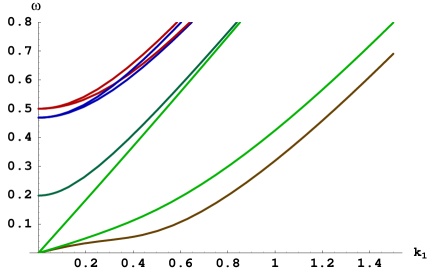
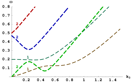
Figure 1: The energy $\omega$ of the 8 light quasiparticle modes as a function of $k_{1}$ (solid lines, left panel) and $k_{3}$ (dashed lines, right panel). The dispersion relations of two heavy modes are outside the plot range. The energy and momenta are measured in units of $m$. The parameters are $\mu/m=1.1$ and $\phi/m=0.1$

There are the following characteristic features of the spectrum. a) The spectrum with ${\bf k}_{\perp}=0$ (the right panel in Fig. 1) is much more degenerate than that with $k_{3}=0$ (the left panel). This point reflects the fact that the axis of the residual $SO(2)$ symmetry is directed along $k_{3}$. Therefore the states with ${\bf k}_{\perp}=0$ and $k_{3}\neq 0$ are more symmetric than those with ${\bf k}_{\perp}\neq 0$. b) The right panel in Fig. 1 contains two branches with local minima at $k_{3}\sim m$, i.e., roton like excitations. Because there are no such excitations in ungauged model (1) MS ; STV , they occur because of the presence of gauge fields. Since roton like excitations occur in superfluid systems, the present model could be relevant for them. c) The NG and Anderson-Higgs mechanisms are conventional in this system. In particular, the dispersion relations for three NG bosons have the form $\omega\sim k$ for low momenta.

When the value of the chemical potential increases, the values of masses of all massive quasipatricles become of the same order. Otherwise, the characteristic features of the dispersion relations remain the same.

IV Model with global $U(1)_{Y}$ symmetry: $m^{2}<0$ case

Let us now turn to the case with negative $m^{2}$. In this case there is the ground state solution (12) describing spontaneous breakdown of $SU(2)\times U(1)_{Y}$ down to $U(1)_{em}$ and preserving the rotational invariance. In order to describe the spectrum of excitations, we make the expansion in Lagrangian density (3) about this solution. Introducing as before small fluctuations $a^{(a)}_{\mu}$ [i.e., $A^{(a)}_{\mu}=\langle A^{(a)}_{\mu}\rangle+a^{(a)}_{\mu}$] and $\tilde{\varphi}_{1}$ [i.e., $\Phi^{T}=(0,\varphi_{0}+\tilde{\varphi}_{1}/\sqrt{2})]$ and keeping only quadratic fluctuation terms, we obtain:

$${\cal L} \simeq \frac{1}{2}f_{0i}^{(a)}f_{0i}^{(a)}-\frac{1}{4}f_{ij}^{(a)}f_{ij}^{(a)}+2\mu\left(f_{0i}^{(2)}a_{i}^{(1)}-f_{0i}^{(1)}a_{i}^{(2)}\right)+2\mu^{2}\left(a_{i}^{(1)}a_{i}^{(1)}+a_{i}^{(2)}a_{i}^{(2)}\right)+\frac{g^{2}\varphi_{0}^{2}}{4}a_{\mu}^{(a)}a^{\mu(a)}$$ (42)

$$+ \frac{1}{2}\partial_{\mu}\tilde{\varphi}_{1}\partial^{\mu}\tilde{\varphi}_{1}-\frac{1}{2}\left(m^{2}+6\lambda\varphi_{0}^{2}\right)\tilde{\varphi}_{1}^{2}.$$

The analysis of the spectrum of eigenvalues of this quadratic form is straightforward. The dispersion relations for charged vector bosons are:

$$\omega^{2}_{-} = (\sqrt{{\bf k}^{2}+\phi^{2}}+2\mu)^{2},$$ (43)

$$\omega^{2}_{+} = (\sqrt{{\bf k}^{2}+\phi^{2}}-2\mu)^{2},$$ (44)

where $\omega_{+}$ and $\omega_{-}$ are the energies of vector bosons with $Q_{em}=+1$ and $Q_{em}=-1$, respectively. The dispersion relations for the neutral vector boson and neutral scalars are $\mu$ independent:

$$\omega^{2}_{0} = {\bf k}^{2}+\phi^{2},$$ (45)

$$\omega^{2}_{\varphi} = {\bf k}^{2}+4\lambda\varphi_{0}^{2}.$$ (46)

Therefore, the chemical potential leads to splitting the masses of two charged vector bosons. In fact, it is easy to check that the terms with the chemical potential in Lagrangian density (42) look exactly as if the chemical potential $\bar{\mu}=2\mu$ for the electric charge $Q_{em}$ was introduced. In other words, as a result of spontaneous $U(1)_{Y}$ symmetry breaking, the dynamical transmutation of the chemical potential occurs: the chemical potential for hypercharge transforms into the chemical potential for electrical charge. Since the hypercharge of vector bosons equals zero and $\tilde{\varphi}_{1}$ scalar is neutral, this transmutation looks quite dramatic: instead of a nonzero density for scalars, a nonzero density for charged vector boson is generated. (The factor $2$ in $\bar{\mu}=2\mu$ is of course connected with the factor $1/2$ in $Q_{em}=I^{3}+\frac{1}{2}Y$.)

In this phase, the parameter $R_{min}$ (5) equals $\phi^{2}=\frac{g^{2}}{4\lambda}|m^{2}|$, i.e., it coincides with the square of the mass of vector bosons in the theory without chemical potential. Therefore, as the chemical potential $\bar{\mu}^{2}$ becomes larger than $\phi^{2}=R_{min}$, a new phase transition should happen. And since for $\bar{\mu}^{2}=\phi^{2}$ vector bosons with charge $+1$ become gapless [see Eq. (44)], one should expect that this phase transition is triggered by generating a condensate of charged vector bosons.

And such a condensate arises indeed. It is not difficult to check that when $\bar{\mu}^{2}>\bar{\mu}^{2}_{cr}\equiv\frac{g^{2}}{4\lambda}|m^{2}|$ , the ground state solution with ansatz (16) occurs. The parameters $C$, $D$, and $\varphi_{0}$ are determined from Eqs. (21) and (23), respectively. For $\bar{\mu}^{2}>\bar{\mu}^{2}_{cr}$, both expression (23) for $\varphi_{0}$ and expression (21) for $|C|^{2}$ are positive and, for $g^{2}\leq 8\lambda$, this solution corresponds to the global minimum of the potential. The phase transition at the critical value $\bar{\mu}^{2}=\bar{\mu}^{2}_{cr}$ is a second order one . The spectrum of excitations in the supercritical phase with $\bar{\mu}^{2}>\bar{\mu}^{2}_{cr}$ is similar to the spectrum in the case of positive $m^{2}$ and $\mu^{2}>m^{2}$ shown in Fig. 1.

Therefore, for $m^{2}<0$ the breakdown of the initial symmetry is realized in two steps, similarly as it takes place in tumbling gauge theories tumbling . Now we can understand more clearly why in the case of positive $m^{2}$ considered above the breakdown of the initial symmetry is realized in one stage. The point is that in that case vector bosons in the theory without chemical potential are massless. Therefore, while $R_{min}=m^{2}>0$ for the chemical potential for hypercharge, $R_{min}=0$ for the chemical potential connected with electrical charge $Q_{em}$ there. This in turn implies that in that case there is no way for increasing $R_{min}$ through the process of the transmutation of the chemical potential as it happens in the case of negative $m^{2}$. Therefore for $m^{2}>0$ the phase in which both the $U(1)_{em}$ symmmetry and the rotational symmetry are broken occurs at once as $\mu^{2}$ becomes larger than $m^{2}$.

V Model with gauged $U(1)_{Y}$ symmetry

Let us now briefly describe the case with $g^{\prime}\neq 0$. In this case the $U(1)_{Y}$ symmetry is local and one should introduce a source term $B_{0}J_{0}$ in Lagrangian density (3) in order to make the system neutral with respect to hypercharge $Y$. This is necessary since otherwise in the system with a nonzero chemical potential $\mu$ thermodynamic equilibrium could not be established. The value of the background hypercharge density $J_{0}$ [representing very heavy particles] is determined from the condition $\langle{B_{0}}\rangle=0$ Kapusta .

After that, the analysis follows closely to that of the case with $g^{\prime}=0$. Because of the additional vector boson $B_{\mu}$, there are now 12 quasiparticles in the spectrum. The sample of spontaneous $SU(2)\times U(1)_{Y}\times SO(3)$ symmetry breaking is the same as for $g^{\prime}=0$ both for $m^{2}\geq 0$ and $m^{2}<0$, with a tumbling like scenario for the latter. However, for supercritical values of the chemical potential, there are now only two gapless NG modes [the third one is “eaten” by a photon like combination of fields $A^{3}_{\mu}$ and $B_{\mu}$ that becomes massive]. Their dispersion relations in infrared read

$$\omega^{2} \simeq \frac{2\mu-\phi}{2\mu+3\phi}{\bf k}^{2}+O(k_{i}^{4}),$$ (47)

$$\omega^{2} \simeq \frac{2\mu-\phi}{2\mu+3\phi}\left(\frac{\phi}{2\mu}{\bf k}_{\perp}^{2}+k_{3}^{2}\right)+O(k_{i}^{4}).$$ (48)

The rest 10 quasiparticles are gapped. The mass (gap) of the two new states is:

$$\Delta^{2}=\mu\phi+\frac{\phi_{b}^{2}}{2}-\sqrt{\left(\mu\phi-\frac{\phi_{b}^{2}}{2}\right)^{2}+\phi^{2}\phi_{b}^{2}}, [\times 2],$$ (49)

where $\phi_{b}^{2}=(g^{\prime})^{2}\varphi_{0}^{2}/2$ with $\varphi_{0}^{2}$ given in Eq. (23). This gap goes to zero together with $g^{\prime}$, i.e., these two degrees of freedom correspond to two transverse states of massless vector boson $B_{\mu}$ in this limit.

The dispersion relations for 10 massive particles are quite complicated. Therefore we performed numerical calculations to extract the corresponding dispersion relations. They are shown in Fig. 2. Bold and thin lines correspond to double degenerate and nondegenerate modes, respectively. As one can see, the two branches connected with gapless NG modes, contain a roton like excitation at $k_{3}\sim m$. Other characteristic features of the spectrum are also similar to those of the spectrum for the case with $g^{\prime}=0$ shown in Fig. 1.

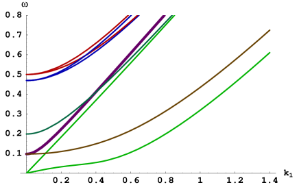
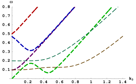
Figure 2: The energy $\omega$ of the 10 light quasiparticle modes as a function of $k_{1}$ (solid lines, left column) and $k_{3}$ (dashed lines, right column). The dispersion relations of two heavy modes are outside the plot ranges. The energy and momenta are measured in units of $m$. The parameters are $\mu/m=1.1$, $\phi/m=0.1$ and $\phi_{b}/m=0.1$.

VI Summary

It would be appropriate to indicate the connection of our results with related results in the literature. The possibility of a condensation of vector bosons in electroweak theory in the presence of a superdense fermionic matter was considered in Ref. linde . This scenario, with some variations, was further studied in Ref. shabad . A possibility of a vector condensation in two-color QCD with a baryon chemical potential was suggested in Ref. lenaghan . Recently, the possibility of a condensation of vector bosons has been studied in a model at finite density that includes only massive vector bosons, with no scalars and fermions sannino . The model is nonrenormalizable and the authors allow independent (i.e., not constrained by gauge invariance) triple and quartic coupling constants. A sample of spontaneous symmetry breaking in that model is very different from that obtained in the present paper.

In conclusion, we studied dynamics in gauged $\sigma$-model at finite density. For positive $m^{2}$, the spontaneous breakdown of $SU(2)\times U(1)_{Y}$ symmetry, caused by a supercritical chemical potential for hypercharge, is always accompanied by spontaneous breakdown of both rotational symmetry $SO(3)$ [down to $SO(2)$] and electromagnetic $U(1)_{em}$. On the other hand, for negative $m^{2}$, the breakdown of $SU(2)\times U(1)_{Y}$ is realized in two stages, with both rotational $SO(3)$ and $U(1)_{em}$ being exact at the first stage. The realization of both the NG mechanism and the Anderson-Higgs mechanism in this model is conventional.

The spectrum of excitations in the model is very rich. In particular, because of the rotational symmetry breakdown, it is anisotropic: the dispersion relations with respect to the longitudinal momentum $k_{3}$ and the transverse momentum ${\bf k}_{\perp}$ are very different. A noticeable point is the existence of excitation branches that behave as phonon like quasiparticles for small momenta and as roton like ones for large longitudinal momenta. This suggests that this model can be relevant for anisotropic superfluid systems.

References

• (1) V. A. Miransky and I. A. Shovkovy, Phys. Rev. Lett. 88, 111601 (2002); hep-ph/0108178.
• (2) T. Schäfer, D. T. Son, M. A. Stephanov, D. Toublan and J. J. Verbaarschot, Phys. Lett. B 522, 67 (2001); hep-ph/0108210.
• (3) P. F. Bedaque and T. Schäfer, Nucl. Phys. A 697, 802 (2002); D. B. Kaplan and S. Reddy, Phys. Rev. D 65, 054042 (2002).
• (4) H. B. Nielsen and S. Chadha, Nucl. Phys. B 105, 445 (1976).
• (5) E. M. Lifshitz and L. P. Pitaevskii, Statistical Physics, Part 2 (Pergamon, New York, 1980); G. E. Volovik, Exotic Properties of Superfluid 3He (World Scientific, Singapore, 1992).
• (6) S. Raby, S. Dimopoulos and L. Susskind, Nucl. Phys. B 169, 373 (1980); V. P. Gusynin, V. A. Miransky and Y. A. Sitenko, Phys. Lett. B 123, 407 (1983).
• (7) L. D. Landau and E. M. Lifshits, Statistical Physics (Pergamon, New York, 1980).
• (8) J. I. Kapusta, Phys. Rev. D 24, 426 (1981).
• (9) H. E. Haber and H. A. Weldon, Phys. Rev. D 25, 502 (1982).
• (10) S. Coleman and E. Weinberg, Phys. Rev. D 7, 1888 (1973).
• (11) A. D. Linde, Phys. Lett. 86B, 39 (1979); I. Krive, Sov. Phys. JETP 56, 477 (1982) [Zh. Eksp. Teor. Fiz. 83, 849 (1982)].
• (12) E. J. Ferrer, V. de la Incera, and A. E. Shabad, Phys. Lett. B 185, 407 (1987); Nucl. Phys. B 309, 120 (1988); J. I. Kapusta, Phys. Rev. D 42, 919 (1990).
• (13) J. T. Lenaghan, F. Sannino and K. Splittorff, Phys. Rev. D 65, 054002 (2002).
• (14) F. Sannino and W. Schäfer, Phys. Lett. B 527, 142 (2002); F. Sannino, Phys. Rev. D 67, 054006 (2003).