Radiation and self-polarization of neutral fermions in quasi-classical description

Abstract

A Lorentz invariant formalism for quasi-classical description of electromagnetic radiation from a neutral spin ${\raise 3.01385pt\hbox{${\scriptstyle 1}$}\!\mathord{\left/{\vphantom{{1}{2}}}\right.\kern-1.2pt}\!\lower 3.01385pt\hbox{${\scriptstyle 2}$}}$ particle with an anomalous magnetic moment moving in an external electromagnetic field is developed. In the high symmetry fields, for which analytical solutions to the Bargmann–Michel–Telegdi equation are known, the so called self-polarization axes, i. e. directions of preferred polarization of particles in the radiation process, are found. Expressions for the radiative transition probability and spectral-angular distribution of the radiation emitted by a polarized particle are obtained in the fields under consideration.

1 Introduction

Electromagnetic radiation from an uncharged spin ${\raise 3.01385pt\hbox{${\scriptstyle 1}$}\!\mathord{\left/{\vphantom{{1}{2}}}\right.\kern-1.2pt}\!\lower 3.01385pt\hbox{${\scriptstyle 2}$}}$ particle with an anomalous magnetic moment moving in certain types of classical electromagnetic field was studied previously within the Furry picture of quantum electrodynamics (QED) [1, 2, 3, 4, 5, 6, 7, 8]. Meanwhile it was observed that under certain conditions the radiation process may be described in purely classical terms using the Bargmann–Michel–Telegdi (BMT) spin evolution equation [9, 10]. In such a pseudoclassical treatment the radiation power is given by the well-known formula for a magnetic moment radiation [12]:

$$\frac{dI}{d{O}}=-\frac{1}{4\pi(lu)^{5}u^{0}}\{{{\ddot{\mu}}^{\nu}}{{\ddot{\mu}}_{\nu}}(ul)^{2}+(l^{\nu}{\ddot{\mu}}_{\nu})^{2}\},$$ (1)

where $\mu^{\nu}$ is the 4-vector of the magnetic moment and $u^{\nu}$ is the 4-velocity of the particle. Here $l^{\nu}=\{1,{\bf l}\},$ where ${\bf l}$ is the unit vector in the direction of an emitted wave; a dot denotes the differentiation with respect to the proper time $\tau$. We use the units $\hbar=c=1$.

The radiation power calculated within the framework of QED is found to correspond to the result obtained from equation (1) under the conditions of quasi-classical character of the motion, namely, that the binding energy due to the magnetic moment in the rest frame should be much smaller than the particle mass, and the external field should vary slowly at the distances of the order of the Compton length, which amounts to the conditions:

$$\mu_{0}{H_{0}}\ll mc^{2},\quad{\hbar\dot{H}_{0}}/{mc^{2}H_{0}}\ll 1,$$ (2)

where $H_{0}$ is the magnetic field strength in the rest frame and $\mu_{0}$ is the value of particle magnetic moment (here we use Gaussian units).

In our papers [13, 14] radiation of unpolarized neutral particles was investigated in quasi-classical approach in the case of arbitrary field. To study radiation from an unpolarized particle one must impose an additional requirement that consists in averaging over the initial spin states and summing over the final polarizations. The averaging of the quantum transition amplitudes should correspond to the averaging over the initial orientations of the magnetic dipole moment within the quasi-classical consideration. We proposed [13, 14] to replace the magnetic moment by

$$\mu^{\nu}=\mu_{0}S^{\nu},$$ (3)

where $S^{\nu}$ is the mean value of the spin vector, its evolution being described by the BMT equation [15]:

$$\dot{S}^{\nu}=2\mu_{0}\{F^{\nu\alpha}S_{\alpha}-u^{\nu}(u_{\alpha}F^{\alpha\beta}S_{\beta})\}.$$ (4)

The validity of this equation is ensured by the conditions (2) [16, 17].

Our main goal was to show that when the averaging over polarization states at $\tau=\tau_{0}$ is performed, the resulting expression for the radiation power depends only on the external field intensity and thus is valid in the case of arbitrary external field subjected to the conditions (2). It is important that the neutral particle moves with a constant velocity in the external field. Of course, the true quantum description of radiation demands the accounting of quantum recoil in the photon emission process. But when conditions (2) are satisfied, the energies of emitted photons are small, therefore we can neglect the change of the particle velocity.

Unfortunately, while studying radiation of polarized particles, even with the assumptions similar to ones discussed above, the approach based on formula (1) is valid only for the transitions without spin-flip. So here we will use another method [18] based on the introduction of quasi-classical spin wave functions in QED formulas.

Such wave functions can be constructed as follows [19]. Suppose the Lorentz equation is solved, i.e. the dependence of coordinates of the particle on proper time is found. Then BMT equation transforms to ordinary differential equation, resolvent of which determines a one-parametric subgroup of the Lorentz group. The quasi-classical spin wave function signifies a spin-tensor, whose evolution is determined by the same one-parametric subgroup.

It is easy to verify that for a neutral particle with spin ${\raise 3.01385pt\hbox{${\scriptstyle 1}$}\!\mathord{\left/{\vphantom{{1}{2}}}\right.\kern-1.2pt}\!\lower 3.01385pt\hbox{${\scriptstyle 2}$}}\,,$ represented by a Dirac bispinor, the equation for the wave function $\Psi(\tau)$ under consideration is [19]

$$\dot{\Psi}=i\mu_{0}\gamma^{5}H^{\mu\nu}u_{\nu}\gamma_{\mu}\hat{u}\,\Psi,$$ (5)

where $H^{\mu\nu}=-\,{\raise 3.01385pt\hbox{${\scriptstyle 1}$}\!\mathord{\left/{\vphantom{{1}{2}}}\right.\kern-1.2pt}\!\lower 3.01385pt\hbox{${\scriptstyle 2}$}}e^{\mu\nu\rho\lambda}F_{\rho\lambda}$ is the dual electromagnetic tensor. Obviously, the density matrix of partially polarized fermion takes the form

$$\rho(\tau,\tau^{\prime})=\frac{1}{2}\,U(\tau,\tau_{0})\big{(}\hat{p}(\tau_{0})+m\big{)}\big{(}1-\gamma^{5}\hat{S}(\tau_{0})\big{)}U^{-1}(\tau^{\prime},\tau_{0}),$$ (6)

where $U(\tau,\tau_{0})$ is the resolvent of equation (5). For a pure state the density matrix reduces to direct product of bispinors, normalized by the condition $\bar{\Psi}(\tau)\Psi(\tau)=2m.$

2 General relations

Now let us investigate the radiation of polarized particles on the base of the above considerations. The formula of quantum electrodynamics which describes the transition probability of a neutral fermion under spontaneous radiation in external field is:

$$\begin{array}[]{ll}\displaystyle P\!\!\!&=\displaystyle-\!\!\int\!\!d^{4}x\,d^{4}y\!\int\frac{d^{4}p\,d^{4}q\,d^{4}k}{(2\pi)^{6}}\,\delta(k^{2})\,\delta(p^{2}-m^{2})\,\delta(q^{2}-m^{2})\\[10.0pt] &\quad\times\varrho^{\mu\nu}_{ph}(x,y;k)\>{\mathrm{Sp}}\big{\{}\Gamma_{\mu}(x)\varrho_{i}(x,y;p)\Gamma_{\nu}(y)\varrho_{f}(y,x;q)\big{\}}.\end{array}$$ (7)

Here $\varrho_{i}(x,y;p),\;\varrho_{f}(y,x;q)$ are density matrices of initial $(i)$ and final $(f)$ states of the fermion, $\,\varrho^{\mu\nu}_{ph}(x,y;k)$ is density matrix of the radiated photon, $\Gamma^{\mu}=-\,\sqrt{4\pi}\mu_{0}\sigma^{\mu\nu}k_{\nu}$ is the vertex function.

In order to pass to the quasi-classical approximation, it is necessary to substitute precise density matrices for the ones constructed in [19] (see (6)) and to neglect the recoil in the photon emission process. The latter operation implies inserting the following expression:

$$(2\pi)^{3}\,\frac{p^{0}q^{0}}{m^{2}}\int\!\!\!\int\!d\tau d\tau^{\prime}\delta^{4}(x^{\alpha}-u^{\alpha}\tau)\delta^{4}(y^{\beta}-u^{\beta}\tau^{\prime})\delta({\bf{p}}-m{\bf{u}})\delta({\bf{q}}-m{\bf{u}}),$$ (8)

in the integrand of (7), which reduces the integration to the particle trajectory. After summation over photon polarizations and integration with respect to fermion momenta and coordinates, we obtain the quasi-classical expressions for the transition probability under investigation:

$$P=\frac{\mu_{0}^{2}}{(2\pi)^{2}}\int\!\!dO\!\!\int\limits_{0}^{\infty}\!k^{3}dk\!\int\!\!\!\int\!d\tau d\tau^{\prime}e^{ik(lu)(\tau-\tau^{\prime})}\,T(\tau,\tau^{\prime};u),$$ (9)

and for the radiation energy

$${\mathcal{E}}=\frac{\mu_{0}^{2}}{(2\pi)^{2}}\int\!\!dO\!\!\int\limits_{0}^{\infty}\!k^{4}dk\!\int\!\!\!\int\!d\tau d\tau^{\prime}e^{ik(lu)(\tau-\tau^{\prime})}\,T(\tau,\tau^{\prime};u).$$ (10)

Here the following notation is introduced:

$$T(\tau,\tau^{\prime};u)=\left(V_{i}V_{f}-A_{i}A_{f}\right),$$ (11)

where $V_{if},A_{if}$ are determined by formulas:

$$\begin{array}[]{l}\displaystyle V_{i}=\frac{1}{4}{\mathrm{Sp}}\!\left\{\hat{l}\,U(\tau)(1+\hat{u})(1\!-\gamma^{5}{\hat{S}}_{0i})U^{-1}(\tau^{\prime})\right\}\!,\\[12.0pt] \displaystyle V_{f}=\frac{1}{4}{\mathrm{Sp}}\!\left\{\hat{l}\,U(\tau^{\prime})(1+\hat{u})(1\!-\gamma^{5}{\hat{S}}_{0f})U^{-1}(\tau)\right\}\!,\\[12.0pt] \displaystyle A_{i}=\frac{1}{4}{\mathrm{Sp}}\Big{\{}\!\gamma^{5}\hat{l}\,U(\tau)(1+\hat{u})(1\!-\gamma^{5}{\hat{S}}_{0i})U^{-1}(\tau^{\prime})\Big{\}},\\[12.0pt] \displaystyle A_{f}=\frac{1}{4}{\mathrm{Sp}}\Big{\{}\!\gamma^{5}\hat{l}\,U(\tau^{\prime})(1+\hat{u})(1\!-\gamma^{5}{\hat{S}}_{0f})U^{-1}(\tau)\Big{\}}.\end{array}$$ (12)

In formulas (9) and (10) the operator $U(\tau)\equiv U(\tau,\tau_{0})$ is the resolvent of the equation (5). Naturally, the spectral-angular distributions for the transition probability and radiation energy can be obtained only if the solution of the equation (5) is known. So first of all we concentrate on investigating the general properties of these physical values.

Let us introduce to the integration variable $k^{\prime}=k(lu)$ which denotes the photon energy in the rest frame of the radiating particle. Using formulas for the Fourier transforms of generalized functions (for example, see [20]), we integrate (9) and (10) with respect to variable $k^{\prime}.$ As a result, we obtain

$$P=\frac{\mu_{0}^{2}}{(2\pi)^{2}}\int\!\frac{dO}{(lu)^{4}}\!\int\!\!\!\int\!d\tau d\tau^{\prime}\frac{1}{2(\tau\!-\tau^{\prime}\!+i0)}(\partial_{\tau}\partial_{\tau^{\prime}}^{2}-\partial_{\tau}^{2}\partial_{\tau^{\prime}})T(\tau,\tau^{\prime};u),$$ (13)

$${\mathcal{E}}=\frac{\mu_{0}^{2}}{(2\pi)^{2}}\int\!\frac{dO}{(lu)^{5}}\!\int\!\!\!\int\!d\tau d\tau^{\prime}\frac{i}{(\tau\!-\tau^{\prime}\!+i0)}\partial_{\tau}^{2}\partial_{\tau^{\prime}}^{2}\,T(\tau,\tau^{\prime};u).$$ (14)

The expressions (13) and (14) could be integrated with respect to the angular variables. As $U(\tau)$ is the resolvent of the equation (5), one has

$$\begin{array}[]{l}\displaystyle\int\!\frac{dO}{(lu)^{4}}\,T(\tau,\tau^{\prime};u)\rightarrow\frac{16\pi}{3}\tilde{V}_{i}\tilde{V}_{f},\\[12.0pt] \displaystyle\int\!\frac{dO}{(lu)^{5}}\,T(\tau,\tau^{\prime};u)\rightarrow\frac{16\pi}{3}u^{0}\tilde{V}_{i}\tilde{V}_{f},\end{array}$$ (15)

where

$$\begin{array}[]{l}\displaystyle\tilde{V}_{i}=\frac{1}{4}{\mathrm{Sp}}\left\{U(\tau)(1-\gamma^{5}{\hat{S}}_{0i})U^{-1}(\tau^{\prime})\right\},\\[12.0pt] \displaystyle\tilde{V}_{f}=\frac{1}{4}{\mathrm{Sp}}\left\{U(\tau^{\prime})(1-\gamma^{5}{\hat{S}}_{0f})U^{-1}(\tau)\right\}.\end{array}$$ (16)

Thus

$$P=\frac{4\mu_{0}^{2}}{3\pi}\!\int\!\!\!\int\!d\tau d\tau^{\prime}\frac{1}{2(\tau\!-\tau^{\prime}\!+i0)}(\partial_{\tau}\partial_{\tau^{\prime}}^{2}-\partial_{\tau}^{2}\partial_{\tau^{\prime}})\tilde{V}_{i}\tilde{V}_{f},$$ (17)

$${\mathcal{E}}=\frac{4\mu_{0}^{2}u^{0}}{3\pi}\!\int\!\!\!\int\!d\tau d\tau^{\prime}\frac{i}{(\tau\!-\tau^{\prime}\!+i0)}\,\partial_{\tau}^{2}\partial_{\tau^{\prime}}^{2}\tilde{V}_{i}\tilde{V}_{f}.\qquad$$ (18)

Obviously, function $T(\tau,\tau^{\prime};u)$ does not vary if $\tau\leftrightarrow\tau^{\prime}$ and $S^{\mu}_{0i}\leftrightarrow S^{\mu}_{0f}.$ It gives the possibility to obtain the following expressions for the angular distribution

$$\frac{dI}{dO}\Big{|}_{S_{0i}\rightarrow S_{0f}}\!+\frac{dI}{dO}\Big{|}_{S_{0f}\rightarrow S_{0i}}=\frac{\mu_{0}^{2}}{2\pi u^{0}(lu)^{5}}\,\partial_{\tau}^{2}\partial_{\tau^{\prime}}^{2}\,T(\tau,\tau^{\prime};u)\Big{|}_{\tau=\tau^{\prime}}\,,$$ (19)

and for the total radiation power

$$I_{S_{0i}\rightarrow S_{0f}}+I_{S_{0f}\rightarrow S_{0i}}=\frac{8\mu_{0}^{2}}{3}\,\partial_{\tau}^{2}\partial_{\tau^{\prime}}^{2}\,\tilde{V}_{i}\tilde{V}_{f}\Big{|}_{\tau=\tau^{\prime}}\,.$$ (20)

If we denote the solutions of BMT equation with initial conditions $S^{\mu}_{i}(\tau_{0})=S^{\mu}_{0i}$ and $S^{\mu}_{f}(\tau_{0})=S^{\mu}_{0f}$ as $S^{\mu}_{i}$ and $S^{\mu}_{f}$ we obtain

$$\begin{array}[]{l}\displaystyle\frac{dI}{dO}\Big{|}_{S_{0i}\rightarrow S_{0f}}\!+\frac{dI}{dO}\Big{|}_{S_{0f}\rightarrow S_{0i}}\\[4.0pt] \displaystyle=\frac{\mu_{0}^{2}}{2\pi u^{0}(lu)^{5}}\Big{\{}2(lu)^{2}\big{[}4H^{2}\big{(}(H^{2})\\[4.0pt] +(HS_{i})(HS_{f})\big{)}-\big{(}{\dot{H}}^{2}+({\dot{H}}S_{i})({\dot{H}}S_{f})\big{)}\big{]}\\[4.0pt] -4(lu)\big{[}(HS_{i})e_{\mu\nu\rho\lambda}l^{\mu}{\dot{H}}^{\nu}H^{\rho}S_{f}^{\lambda}+(HS_{f})e_{\mu\nu\rho\lambda}l^{\mu}{\dot{H}}^{\nu}H^{\rho}S_{i}^{\lambda}\big{]}\\[4.0pt] -2\big{[}\big{(}4H^{2}(Hl)^{2}-({\dot{H}}l)^{2}\big{)}+4H^{2}(Hl)e_{\mu\nu\rho\lambda}l^{\mu}{\dot{H}}^{\nu}u^{\rho}H^{\lambda}\big{]}\\[2.0pt] -2\big{[}(lS_{i})(lS_{f})\big{(}4(H^{2})^{2}+{\dot{H}}^{2}\big{)}+8(Hl)^{2}(HS_{i})(HS_{f})\big{]}\\[4.0pt] +8H^{2}(Hl)\big{[}(lS_{i})(HS_{f})+(lS_{f})(HS_{i})\big{]}\\[4.0pt] +2({\dot{H}}l)\big{[}(lS_{i})({\dot{H}}S_{f})+(lS_{f})({\dot{H}}S_{i})\big{]}\\[4.0pt] -4H^{2}\big{[}(lS_{i})e_{\mu\nu\rho\lambda}l^{\mu}{\dot{H}}^{\nu}u^{\rho}S_{f}^{\lambda}+(lS_{f})e_{\mu\nu\rho\lambda}l^{\mu}{\dot{H}}^{\nu}u^{\rho}S_{i}^{\lambda}\big{]}\\[4.0pt] -8H^{2}e_{\mu\nu\rho\lambda}l^{\mu}{{H}}^{\nu}u^{\rho}S_{i}^{\lambda}\,e_{\mu\nu\rho\lambda}l^{\mu}{{H}}^{\nu}u^{\rho}S_{f}^{\lambda}\\[4.0pt] -2e_{\mu\nu\rho\lambda}l^{\mu}{\dot{H}}^{\nu}u^{\rho}S_{i}^{\lambda}\,e_{\mu\nu\rho\lambda}l^{\mu}{\dot{H}}^{\nu}u^{\rho}S_{f}^{\lambda}\\ -4\big{(}(lS_{i})(H{\dot{H}})-(Hl)({\dot{H}}S_{i})-({\dot{H}}l)(HS_{i})\big{)}e_{\mu\nu\rho\lambda}l^{\mu}{{H}}^{\nu}u^{\rho}S_{f}^{\lambda}\\[4.0pt] -4\big{(}(lS_{f})(H{\dot{H}})-(Hl)({\dot{H}}S_{f})-({\dot{H}}l)(HS_{f})\big{)}e_{\mu\nu\rho\lambda}l^{\mu}{{H}}^{\nu}u^{\rho}S_{i}^{\lambda}\Big{\}},\end{array}$$ (21)

$$\begin{array}[]{l}I_{S_{0i}\rightarrow S_{0f}}+I_{S_{0f}\rightarrow S_{0i}}\\[4.0pt] =\displaystyle\frac{16}{3}\,\mu_{0}^{2}\Big{\{}4H^{2}\big{(}(H^{2})+(HS_{i})(HS_{f})\big{)}-\big{(}{\dot{H}}^{2}+({\dot{H}}S_{i})({\dot{H}}S_{f})\big{)}\\ -2\big{[}(HS_{i})e_{\mu\nu\rho\lambda}u^{\mu}{\dot{H}}^{\nu}H^{\rho}S_{f}^{\lambda}+(HS_{f})e_{\mu\nu\rho\lambda}u^{\mu}{\dot{H}}^{\nu}H^{\rho}S_{i}^{\lambda}\big{]}\Big{\}},\end{array}$$ (22)

where $H^{\mu}$ denotes $\mu_{0}H^{\mu\nu}u_{\nu}.$ If we average over the initial spin states and summarize over the final ones in expressions (21) and (22), for which purpose we must set $S^{\mu}_{i}=S^{\mu}_{f}=0,$ we obtain the angular distribution and total radiation power of unpolarized fermion [13, 14]. If we set $S^{\mu}_{i}=S^{\mu}_{f}=S^{\mu}$ in formulas (21) and (22) and divide the obtained expression by $2,$ we obtain the angular distribution and total radiation power without spin flip. One can see that the radiation powers without spin flip are equal for the states of the particle with opposite polarizations.

Using the above technique, we obtain for the transition probability at the time moment $t$:

$$\begin{array}[]{l}\displaystyle\frac{dW}{dO}\Big{|}_{S_{0i}\rightarrow S_{0f}}\!\!-\frac{dW}{dO}\Big{|}_{S_{0f}\rightarrow S_{0i}}\\[8.0pt] =\displaystyle\frac{\mu_{0}^{2}}{4\pi u^{0}(lu)^{4}}\Big{\{}4\big{(}(HS_{i})-(HS_{f})\big{)}\big{(}H^{2}(lu)^{2}-(Hl)^{2}\big{)}\\[4.0pt] -(lu)e_{\mu\nu\rho\lambda}l^{\mu}{\dot{H}}^{\nu}H^{\rho}(S_{i}^{\lambda}-S_{f}^{\lambda})+\big{(}(lS_{i})-(lS_{f})\big{)}e_{\mu\nu\rho\lambda}l^{\mu}{\dot{H}}^{\nu}{H}^{\rho}u^{\lambda}\\[4.0pt] -(Hl)e_{\mu\nu\rho\lambda}l^{\mu}{\dot{H}}^{\nu}u^{\rho}(S_{i}^{\lambda}-S_{f}^{\lambda})+(\dot{H}l)e_{\mu\nu\rho\lambda}l^{\mu}{H}^{\nu}u^{\rho}(S_{i}^{\lambda}-S_{f}^{\lambda})\Big{\}},\end{array}$$ (23)

$$\begin{array}[]{l}W_{S_{0i}\rightarrow S_{0f}}-W_{S_{0f}\rightarrow S_{0i}}\\[4.0pt] =\displaystyle\frac{4\mu_{0}^{2}}{3u^{0}}\Big{\{}4H^{2}\big{(}(HS_{i})-(HS_{f})\big{)}-e_{\mu\nu\rho\lambda}u^{\mu}{\dot{H}}^{\nu}H^{\rho}(S_{i}^{\lambda}-S_{f}^{\lambda})\Big{\}}.\end{array}$$ (24)

Let us define the state of total self-polarization $S^{\mu}_{0tp}$ by either of the two equivalent conditions

$$I_{S_{0tp}\rightarrow\,-S_{0tp}}=0,\qquad W_{S_{0tp}\rightarrow\,-S_{0tp}}=0.$$ (25)

In the general case, in this state $I_{S_{0tp}\rightarrow S_{0tp}}\neq 0.$ If the state of total self-polarization $S^{\mu}_{0tp}$ is known, then radiation power of the particle in $-S^{\mu}_{0tp}$ state is

$$\begin{array}[]{ll}I_{-S_{0tp}}\!\!\!&=\displaystyle\frac{8}{3}\,\mu_{0}^{2}\Big{\{}4H^{2}\big{(}3H^{2}-(HS_{tp})^{2}\big{)}-\big{(}3{\dot{H}}^{2}-(\dot{H}S_{tp})^{2}\big{)}\\[4.0pt] &+\,4(HS_{tp})e_{\mu\nu\rho\lambda}u^{\mu}{\dot{H}}^{\nu}H^{\rho}S_{tp}^{\lambda}\Big{\}}.\end{array}$$ (26)

Underline that the obtained expressions do not allow to decide, which state of the particle is the state with maximum possible radiative self-polarization, also what is the self-polarization degree, and whether the state of total self-polarization exists. This is due to the fact that in the general case the quantity $W_{S_{0}\rightarrow-S_{0}}+W_{-S_{0}\rightarrow S_{0}}$ necessary for obtaining the balance equation (see, for example, [21]) could not be expressed in terms of solutions to the BMT equation.

However, we can show that there always exists either the total self-polarization state, or the state with maximum possible self-polarization for a neutral fermion moving in an external field, provided that this field belongs to a class of fields admitted, on one hand, by the requirement that equation (5) and consequently BMT equation should allow precise analytical solutions, and, on the other hand, specified by conditions of solvability that do not depend on the magnitude of the anomalous moment $\mu_{0}$. The latter can become the total self-polarization state under continuous variation of the field characteristics.

3 Radiation and self-polarization in the fields of special type

Let us prove the above statement. The conditions for the existence of analytical solutions of BMT equation and their form are given in [22]. Using the results of [22], in order to obtain the solutions of (5), we introduce the following basis vectors:

$$\begin{array}[]{l}\displaystyle n^{\mu}_{0}=u^{\mu},\quad n^{\mu}_{1}=H^{\mu}/\sqrt{-H^{2}},\\[3.0pt] \displaystyle n^{\mu}_{2}={\big{(}H^{\mu}{(H\dot{H})}-\dot{H}^{\mu}H^{2}\big{)}}/{\sqrt{-H^{2}N}},\\[3.0pt] \displaystyle n^{\mu}_{3}=-\,e^{\mu\nu\rho\lambda}u_{\nu}H_{\rho}{\dot{H}}_{\lambda}/\sqrt{N},\end{array}$$ (27)

where

$$N={H^{2}{\dot{H}}^{2}-(H\dot{H})^{2}}.$$ (28)

This basis is orthogonal and its elements satisfy the system of equations, which is a four-dimensional generalization of the Frenet equations:

$${\dot{n}}^{\mu}_{1}=\kappa n^{\mu}_{2},\qquad{\dot{n}}^{\mu}_{2}=\varkappa n^{\mu}_{3}-\kappa n^{\mu}_{1},\qquad{\dot{n}}^{\mu}_{3}=-\varkappa n^{\mu}_{2}.$$ (29)

Here parameters $\kappa$ and $\varkappa$ are analogs of curvature and torsion:

$$\kappa=\frac{N^{1/2}}{(-H^{2})},\qquad\varkappa={\frac{\displaystyle\sqrt{-H^{2}}}{N}}e^{\alpha\beta\gamma\delta}{\ddot{H}_{\alpha}}{\dot{H}_{\beta}}H_{\gamma}u_{\delta}.$$ (30)

In the chosen basis the spin vector is of the form

$$S^{\mu}=\sum^{3}_{i=1}S_{i}n_{i}^{\mu},$$

where $S_{i}=-(Sn_{i})$ are components of three-dimensional spin vector $\mathbf{S}.$

The $\mathbf{S}$ components satisfy the set of equations

$$\begin{array}[]{l}\displaystyle\dot{S}_{1}=\kappa S_{2},\\[2.0pt] \displaystyle\dot{S}_{2}=\big{(}\varkappa-2\sqrt{-H^{2}}\;\big{)}S_{3}-\kappa S_{1},\\[2.0pt] \displaystyle\dot{S}_{3}=-\big{(}\varkappa-2\sqrt{-H^{2}}\;\big{)}S_{2}.\end{array}$$ (31)

Let us define $N_{i}=\gamma^{5}\hat{n}_{i}\hat{u}.$ Obviously $N_{i}N_{j}=-ie_{ijk}N_{k},$ $\bar{N}_{i}={N}_{i}.$ Using standard transition from spinor to bispinor representation [24], we obtain from formulas [22]

$$\begin{array}[]{l}U=VR_{0},\\[4.0pt] \displaystyle V=\cos\frac{\Omega_{0}}{2}+i({\bf Nt}_{0})\sin\frac{\Omega_{0}}{2}\,,\\[8.0pt] \displaystyle R_{0}=\cos\frac{\Omega}{2}-i({\bf Nt})\sin\frac{\Omega}{2}\,.\end{array}$$ (32)

Here

$$\begin{array}[]{l}\displaystyle{\bf t}_{0}=\big{\{}\eta_{\varkappa},\,0,\,\eta_{\kappa}\big{\}}\big{(}\eta_{\varkappa}^{2}+\eta_{\kappa}^{2}\big{)}^{-1/2},\\[3.0pt] \displaystyle\Omega_{0}=\big{(}\eta_{\varkappa}^{2}+\eta_{\kappa}^{2}\big{)}^{1/2}\!\int\limits_{\tau_{0}}^{\tau}\!\sqrt{-H^{2}}\,d\tau,\\[4.0pt] {\bf t}=\big{\{}\eta_{\varkappa}-2,\,0,\,\eta_{\kappa}\big{\}}\big{(}(\eta_{\varkappa}-2)^{2}+\eta_{\kappa}^{2}\big{)}^{-1/2},\\[3.0pt] \displaystyle\Omega=\big{(}(\eta_{\varkappa}-2)^{2}+\eta_{\kappa}^{2}\big{)}^{1/2}\!\int\limits_{\tau_{0}}^{\tau}\!\sqrt{-H^{2}}\,d\tau,\end{array}$$ (33)

where

$$\eta_{\varkappa}=\frac{\varkappa}{\sqrt{-H^{2}}}={\mathrm{const}},\qquad\eta_{\kappa}=\frac{\kappa}{\sqrt{-H^{2}}}={\mathrm{const}}.$$ (34)

The meaning of the introduced vectors ${\bf{t}}_{0}$ and ${\bf{t}}$ is quite evident. The vector ${\bf{t}}_{0}$ represents the axis about which the trihedron determining the field orientation in the rest frame of the particle rotates (i. e. the Darboux vector). Vector ${\bf{t}}$ defines the axis about which the spin vector precesses in the particle rest frame.

Note that, if the conditions (34) are satisfied, the vector ${\bf{t}}$ is the only constant solution of the system (31). The corresponding solution of BMT equation is:

$$\begin{array}[]{ll}\displaystyle S^{\mu}\!\!\!&=\left[H^{\mu}\big{(}\varkappa-2\sqrt{-H^{2}}\;\big{)}/\sqrt{-H^{2}}\right.-\,e^{\mu\nu\rho\lambda}u_{\nu}\left.H_{\rho}{\dot{H}}_{\lambda}\,{\kappa}/\sqrt{N}\right]\\ &\times\displaystyle\left[\big{(}\varkappa-2\sqrt{-H^{2}}\;\big{)}^{2}+{\kappa}^{2}\right]^{-1/2}.\end{array}$$ (35)

Characteristic of this solution is that the spin vector (35) retains the orientation with respect to the external field. As we shall see later, it is precisely this vector that fixes the direction of the self-polarization axis.

Inserting (30) into (16), we obtain

$$\begin{array}[]{ll}\displaystyle\tilde{V}_{i}\!\!\!&=\displaystyle\left\{\cos\frac{\Omega-\Omega^{\prime}}{2}+i({\bf{tS}}_{0i})\sin\frac{\Omega-\Omega^{\prime}}{2}\right\}\cos\frac{\Omega_{0}-\Omega^{\prime}_{0}}{2}\\ &\displaystyle+\left\{({\bf{tt}}_{0})\sin\frac{\Omega-\Omega^{\prime}}{2}-i\bigg{[}({\bf{tt}}_{0})({\bf{tS}}_{0i})\cos\frac{\Omega-\Omega^{\prime}}{2}\right.\\ &+\left.\displaystyle\big{(}({\bf S}_{0i}{\bf t})-({\bf{tt}}_{0})({\bf{tS}}_{0i})\big{)}\cos\frac{\Omega+\Omega^{\prime}}{2}\right.\\ &\left.+\,\,\displaystyle({\bf S}_{0i}[{\bf t}\times{\bf t}_{0}])\,\sin\frac{\Omega+\Omega^{\prime}}{2}\,\,\bigg{]}\right\}\displaystyle\sin\frac{\Omega_{0}-\Omega^{\prime}_{0}}{2}\,.\end{array}$$ (36)

The expression for $\tilde{V}_{f}$ is obtained from (36) after the substitution ${\bf{S}}_{0i}\!\rightarrow\!-\,{\bf{S}}_{0f}.$ If we set ${\bf{S}}_{0i}=\zeta_{i}{\bf{t}}$ and ${\bf{S}}_{0f}=\zeta_{f}{\bf{t}},$ we obtain

$$\begin{array}[]{ll}\displaystyle\!\!\!\!\!\tilde{V}_{i}\tilde{V}_{f}\!\!\!&=\displaystyle\frac{1}{4}e^{i(\Omega-\Omega^{\prime})(\zeta_{i}-\zeta_{f})/2}\\[8.0pt] &\times\displaystyle\left\{\left[e^{i(\Omega_{0}-\Omega^{\prime}_{0})(\zeta_{i}+\zeta_{f})/2}\right.\right.+\left.e^{-i(\Omega_{0}-\Omega^{\prime}_{0})(\zeta_{i}+\zeta_{f})/2}\right]\!\big{(}1-({\bf{tt}}_{0})^{2}\big{)}\\[8.0pt] &\displaystyle+\,e^{i(\Omega_{0}-\Omega^{\prime}_{0})(\zeta_{i}-\zeta_{f})/2}\left(1-({\bf{tt}}_{0})\right)^{2}+\left.e^{-i(\Omega_{0}-\Omega^{\prime}_{0})(\zeta_{i}-\zeta_{f})/2}\left(1+({\bf{tt}}_{0})\right)^{2}\right\}\!.\end{array}$$ (37)

Inserting this expression into (17) and (18), we obtain the transition probability with, as well as without the spin flip, and consequently the total radiation energy. If $\sqrt{-H^{2}}={\mathrm{const}},$ we can obtain final expressions for the above values by locking the integration contour in lower or upper half-plane of the complex variable $\tau-\tau^{\prime}.$ Hence, if $\dot{\Omega}>\dot{\Omega}_{0},$ we obtain the following expression for the transition probability with spin flip :

$$\begin{array}[]{l}\displaystyle W_{\zeta_{i}\rightarrow-\zeta_{i}}=\frac{2\mu_{0}^{2}}{3u^{0}}\,\Big{\{}2(\dot{\Omega})^{3}\left(1-({\bf{tt}}_{0})^{2}\right)+(\dot{\Omega}-\dot{\Omega}_{0})^{3}\left(1+({\bf{tt}}_{0})\right)^{2}\\[8.0pt] \displaystyle\qquad\quad\;\;+\,(\dot{\Omega}+\dot{\Omega}_{0})^{3}\left(1-({\bf{tt}}_{0})\right)^{2}\Big{\}}\Theta(-\zeta_{i}).\end{array}$$ (38)

If $\dot{\Omega}<\dot{\Omega}_{0},$ then

$$\begin{array}[]{l}\displaystyle W_{\zeta_{i}\rightarrow-\zeta_{i}}=\frac{2\mu_{0}^{2}}{3u^{0}}\,\Big{\{}\Big{[}(\dot{\Omega}_{0}-\dot{\Omega})^{3}\left(1+({\bf{tt}}_{0})\right)^{2}\Big{]}\Theta(\zeta_{i})\\[8.0pt] \displaystyle\qquad\quad\;\;+\Big{[}2(\dot{\Omega})^{3}\left(1-({\bf{tt}}_{0})^{2}\right)+(\dot{\Omega}+\dot{\Omega}_{0})^{3}\left(1-({\bf{tt}}_{0})\right)^{2}\Big{]}\Theta(-\zeta_{i})\Big{\}}.\end{array}$$ (39)

Here $\Theta(x)$ is the Heaviside theta-function.

Thus if $\dot{\Omega}>\dot{\Omega}_{0}$ the state with spin vector (35) will be the state with total self-polarization, otherwise it will have partial self-polarization. Using (36), it is easy to verify that the maximum possible degree of self-polarization is obtained in the state (35):

$$\begin{array}[]{l}\displaystyle\frac{W_{\zeta_{p}\rightarrow-\zeta_{p}}-W_{-\zeta_{p}\rightarrow\zeta_{p}}}{W_{\zeta_{p}\rightarrow-\zeta_{p}}+W_{-\zeta_{p}\rightarrow\zeta_{p}}}\\[12.0pt] \displaystyle\!\!\!\!\!\!=\frac{2(\dot{\Omega})^{3}\left(1-({\bf{tt}}_{0})^{2}\right)+(\dot{\Omega}-\dot{\Omega}_{0})^{3}\left(1+({\bf{tt}}_{0})\right)^{2}+(\dot{\Omega}+\dot{\Omega}_{0})^{3}\left(1-({\bf{tt}}_{0})\right)^{2}}{2(\dot{\Omega})^{3}\left(1-({\bf{tt}}_{0})^{2}\right)+{|\dot{\Omega}-\dot{\Omega}_{0}|}^{3}\left(1+({\bf{tt}}_{0})\right)^{2}+(\dot{\Omega}+\dot{\Omega}_{0})^{3}\left(1-({\bf{tt}}_{0})\right)^{2}}\end{array}$$ (40)

The transition probability without spin flip is determined as:

$$W_{\zeta_{i}\rightarrow\zeta_{i}}=\frac{2\mu_{0}^{2}}{3u^{0}}\,\Big{\{}(\dot{\Omega}_{0})^{3}\left(1-({\bf{tt}}_{0})^{2}\right)\Big{\}}.$$ (41)

The total radiation power is

$$\begin{array}[]{ll}\displaystyle I_{\zeta_{i}\rightarrow-\zeta_{i}}\!\!\!&=\displaystyle\frac{2\mu_{0}^{2}}{3}\,\Big{\{}2(\dot{\Omega})^{4}\left(1-({\bf{tt}}_{0})^{2}\right)\\[8.0pt] &\displaystyle+(\dot{\Omega}-\dot{\Omega}_{0})^{4}\left(1+({\bf{tt}}_{0})\right)^{2}+(\dot{\Omega}+\dot{\Omega}_{0})^{4}\left(1-({\bf{tt}}_{0})\right)^{2}\Big{\}}\Theta(-\zeta_{i})\end{array}$$ (42)

if $\dot{\Omega}>\dot{\Omega}_{0}$ and

$$\begin{array}[]{ll}\displaystyle I_{\zeta_{i}\rightarrow-\zeta_{i}}\!\!\!&=\displaystyle\frac{2\mu_{0}^{2}}{3}\,\Big{\{}\Big{[}(\dot{\Omega}_{0}-\dot{\Omega})^{4}\left(1+({\bf{tt}}_{0})\right)^{2}\Big{]}\Theta(\zeta_{i})\\[8.0pt] &\displaystyle+\Big{[}2(\dot{\Omega})^{4}\left(1-({\bf{tt}}_{0})^{2}\right)+(\dot{\Omega}+\dot{\Omega}_{0})^{4}\left(1-({\bf{tt}}_{0})\right)^{2}\Big{]}\Theta(-\zeta_{i})\Big{\}}\end{array}$$ (43)

if $\dot{\Omega}<\dot{\Omega}_{0};$

$$I_{\zeta_{i}\rightarrow\zeta_{i}}\quad=\frac{2\mu_{0}^{2}}{3}\,\Big{\{}(\dot{\Omega}_{0})^{4}\left(1-({\bf{tt}}_{0})^{2}\right)\Big{\}}.$$ (44)

These formulas show that in the fields under investigation, in the rest frame, the particle can radiate photons of only four energies: the ones corresponding to the characteristic frequency of the external field variation, to the frequency of spin precession, and to two combination frequencies, the radiation with the external field frequency being possible only without spin flip.

The obtained formulas may be somewhat simplified using explicit expressions for $\dot{\Omega},\,\dot{\Omega}_{0},\,{\bf{t}}_{0},$ and $\,{\bf{t}}.$ We perform this for special fields.

4 Examples

First of all, we consider the case of constant homogeneous magnetic field. This problem is in a sense a test for calculation techniques. It was first discussed in [1] within the framework of quantum theory, and then was repeatedly investigated using various quasi-classical methods [25] (see, also, [26, 27]). Since in the field under consideration $\kappa=\varkappa=0,$ the integrals over $\tau,\;\tau^{\prime}$ in formulas (9), (10) can be calculated precisely for arbitrary $S_{0i},\;S_{0f}.$ We obtain

$$\begin{array}[]{ll}\displaystyle\frac{dW}{dO\,dk}\Big{|}_{S_{0i}\rightarrow S_{0f}}\!\!\!&=\displaystyle\frac{\mu_{0}^{2}\,k^{3}}{8\pi u^{0}}\;\delta\big{(}k(lu)-2\sqrt{-H^{2}}\;\big{)}\\[12.0pt] &\times\!\displaystyle\left(\!(lu)^{2}-\frac{(Hl)^{2}}{H^{2}}\right)\!\!\left(\!1-\frac{(HS_{0i})}{\sqrt{-H^{2}}}\right)\!\!\left(\!1+\frac{(HS_{0f})}{\sqrt{-H^{2}}}\right)\!,\end{array}$$ (45)

$$\begin{array}[]{ll}\displaystyle\frac{dI}{dO\,dk}\Big{|}_{S_{0i}\rightarrow S_{0f}}\!\!\!&=\displaystyle\frac{\mu_{0}^{2}\,k^{4}}{8\pi u^{0}}\;\delta\big{(}k(lu)-2\sqrt{-H^{2}}\;\big{)}\\[12.0pt] &\times\!\displaystyle\left(\!(lu)^{2}-\frac{(Hl)^{2}}{H^{2}}\right)\!\!\left(\!1-\frac{(HS_{0i})}{\sqrt{-H^{2}}}\right)\!\!\left(\!1+\frac{(HS_{0f})}{\sqrt{-H^{2}}}\right)\!.\end{array}$$ (46)

Obviously, in this case the self-polarization is total, and self-polarization axis is $S^{\mu}_{tp}=-{H^{\mu}}/{\sqrt{-H^{2}}},$ i. e., depending on the sign of anomalous magnetic moment, in the rest frame the particle spin is oriented either along or opposite to the direction of the magnetic field. Because of the relation $\dot{\Omega}_{0}=0,$ the radiation frequency in the rest frame is equal to the frequency of spin precession. It is highly important that, under transition from any spin state, the spectral-angular distribution of the radiation is the same irrespective of whether the spin flip takes place. In this case the classical formula for magnetic dipole radiation is valid only for the transitions without spin flip. However, due to the above feature, the radiation power calculated using this formula differs from the correct value only in numerical coefficient.

After the integration with respect to the angles and photon energies, we obtain

$$W_{S_{0i}\rightarrow S_{0f}}=\frac{16\mu_{0}^{2}}{3u^{0}}\big{(}-H^{2}\big{)}^{3/2}\!\left(\!1-\frac{(HS_{0i})}{\sqrt{-H^{2}}}\right)\!\!\left(\!1+\frac{(HS_{0f})}{\sqrt{-H^{2}}}\right)\!,\\$$ (47)

$$I_{S_{0i}\rightarrow S_{0f}}\;\;=\frac{32\mu_{0}^{2}}{3}\big{(}H^{2}\big{)}^{2}\!\left(\!1-\frac{(HS_{0i})}{\sqrt{-H^{2}}}\right)\!\!\left(\!1+\frac{(HS_{0f})}{\sqrt{-H^{2}}}\right)\!.\!\!\!\!$$ (48)

If we introduce $S_{0i}^{\mu}=\zeta_{i}S^{\mu}_{tp},\;S_{0f}^{\mu}=\zeta_{f}S^{\mu}_{tp}$ and consider the transitions only between those states, we obtain the expressions analogous to the ones derived in [1].

Let us now discuss the radiation in the field of a circularly polarized monochromatic plane wave with the frequency $\omega$ and the amplitude $E.$ In this case

$$\begin{array}[]{ll}H^{\mu}&=-\mu_{0}E\left[\big{(}(nu)a_{1}^{\mu}-(a_{1}u)n^{\mu}\big{)}\cos\omega(nx)\right.\\[4.0pt] &\quad\,+{g}\left.\big{(}a_{2}^{\mu}(nu)-(a_{2}u)n^{\mu}\big{)}\sin\omega(nx)\right],\\[4.0pt] \!\!\!\!\!-H^{2}\!\!\!&=\mu_{0}^{2}(nu)^{2}E^{2},\qquad\kappa=\omega(nu),\qquad\varkappa=0.\end{array}$$ (49)

Here

$$\begin{array}[]{ll}n^{\mu}=\left({1,\;{\bf n}}\right),&\quad n^{\mu}_{+}={\raise 3.01385pt\hbox{${\scriptstyle{1}}$}\!\mathord{\left/{\vphantom{{1}{2}}}\right.\kern-1.2pt}\!\lower 3.01385pt\hbox{${\scriptstyle{2}}$}}\left({1,-\,{\bf n}}\right),\\[4.0pt] a^{\mu}_{1}=\left({0,\;{\bf a}_{1}}\right),&\quad a^{\mu}_{2}=\left({0,\;{\bf a}_{2}}\right),\end{array}$$ (50)

where $\omega{\bf{n}}$ is the wave vector and ${\bf{a}}_{i}$ are the unit vectors of polarization.

Consequently,

$${\dot{\Omega}}_{0}=\omega(nu),\quad{\dot{\Omega}}=\omega(nu)(1+d^{2})^{1/2},\quad({\bf t}{\bf t}_{0})=(1+d^{2})^{-1/2},$$ (51)

where $d=2\mu_{0}E/\omega.$ Since the condition $\dot{\Omega}_{0}<\dot{\Omega}$ is satisfied for any wave parameters, the transition probability is determined by (38) and (41), and radiation power by (42) and (44).

It was indicated above that in the particle rest frame the photons with only four frequencies are radiated. Partial transition probabilities and radiation powers are expressed as

$$\begin{array}[]{ll}\displaystyle W_{\zeta_{i}\rightarrow-\zeta_{i}}(\dot{\Omega})&=\displaystyle\frac{4\mu_{0}^{2}\omega^{3}(nu)^{3}d^{2}}{3u^{0}}\,(1+d^{2})^{1/2}\Theta(-\zeta_{i}),\\[6.0pt] \displaystyle W_{\zeta_{i}\rightarrow-\zeta_{i}}(\dot{\Omega}\pm\dot{\Omega}_{0})\!\!\!&=\displaystyle\frac{2\mu_{0}^{2}\omega^{3}(nu)^{3}d^{4}}{3u^{0}(1+d^{2})}\,\big{(}(1+d^{2})^{1/2}\pm 1\big{)}\Theta(-\zeta_{i}),\\[10.0pt] \displaystyle W_{\zeta_{i}\rightarrow\zeta_{i}}(\dot{\Omega}_{0})&=\displaystyle\frac{2\mu_{0}^{2}\omega^{3}(nu)^{3}d^{2}}{3u^{0}(1+d^{2})}\,;\end{array}$$ (52)

$$\begin{array}[]{ll}\displaystyle I_{\zeta_{i}\rightarrow-\zeta_{i}}(\dot{\Omega})&=\displaystyle\frac{4\mu_{0}^{2}\omega^{4}(nu)^{4}d^{2}}{3}\,(1+d^{2})\Theta(-\zeta_{i}),\\[6.0pt] \displaystyle I_{\zeta_{i}\rightarrow-\zeta_{i}}(\dot{\Omega}\pm\dot{\Omega}_{0})\!\!\!&=\displaystyle\frac{2\mu_{0}^{2}\omega^{4}(nu)^{4}d^{4}}{3(1+d^{2})}\,\big{(}(1+d^{2})^{1/2}\pm 1\big{)}^{2}\Theta(-\zeta_{i}),\\[10.0pt] \displaystyle I_{\zeta_{i}\rightarrow\zeta_{i}}(\dot{\Omega}_{0})&=\displaystyle\frac{2\mu_{0}^{2}\omega^{4}(nu)^{4}d^{2}}{3(1+d^{2})}\,.\end{array}$$ (53)

The fact, that the particle can radiate not only with the frequency of external wave, but also with other three frequencies, which are not multiples of the first one, was mentioned in [4]. We must emphasize, that in our case the self-polarization axis does not determine a constant space direction, but is rigidly tied to the external field. Namely, in the rest frame of the particle its spin vector precesses with the wave frequency around the wave vector, the spin vector being in the same plane with the wave vector and the vector of magnetic field strength, the angle between the spin vector and the wave vector being equal to arc tangent of parameter $d.$

The interesting case is the Redmond field, which is the superposition of the above discussed circularly polarized wave and a constant homogeneous magnetic field directed along its wave vector. Since in the Redmond field the conditions (34) are satisfied only when the particle moves along the constant magnetic field $H_{\parallel},$ we study this case and set $(a_{i}u)=0.$ Then

$$\begin{array}[]{ll}H^{\mu}\!\!\!&=-\mu_{0}E(nu)\big{[}a_{1}^{\mu}\cos\omega(nx)+{g}a_{2}^{\mu}\sin\omega(nx)\big{]}\\[6.0pt] &-\mu_{0}H_{\parallel}\left[n^{\mu}(n_{+}u)-n^{\mu}_{+}(nu)\right],\\[6.0pt] \!\!\!\!\!-H^{2}&=\mu_{0}^{2}\big{(}(nu)^{2}E^{2}+H_{\parallel}^{2}\big{)},\\[6.0pt] \end{array}$$ (54)

$$\kappa=\displaystyle\frac{\omega(nu)}{(1+H_{\parallel}^{2}/E^{2}(nu)^{2})^{1/2}}\,,\qquad\varkappa=-\frac{{g}\mu_{0}\omega H_{\parallel}/|\mu_{0}|E}{(1+H_{\parallel}^{2}/E^{2}(nu)^{2})^{1/2}}\,.$$ (55)

Therefore,

$$\begin{array}[]{ll}\displaystyle{\dot{\Omega}}_{0}&=\omega(nu),\\[6.0pt] {\dot{\Omega}}&=\omega(nu)\big{(}(1+2{g}\mu_{0}H_{\parallel}/\omega(nu))^{2}+d^{2}\big{)}^{1/2},\\[6.0pt] \displaystyle\!\!\!\!({\bf{tt}}_{0})\!\!&=\displaystyle\frac{1+2{g}\mu_{0}H_{\parallel}/\omega(nu)}{\big{(}(1+2g\mu_{0}H_{\parallel}/\omega(nu))^{2}+d^{2}\big{)}^{1/2}}\,.\end{array}$$ (56)

If $\varkappa<\sqrt{-H^{2}},$ then the condition $\dot{\Omega}_{0}<\dot{\Omega}$ is satisfied. In this case, the transition probability is defined by (38) and (41), and the radiation power is defined by (42) and (44).

If $\varkappa>\sqrt{-H^{2}},$ then the condition $\dot{\Omega}_{0}>\dot{\Omega}$ is satisfied. In this case the transition probability is defined by (39) and (41), whereas the radiation power is determined by (43) and (44). For this situation to take place, it is necessary that $d\leqslant 1$ and, consequently, the constant magnetic field strength should satisfy the condition:

$$q_{1}<-2{g}\mu_{0}H_{\parallel}/\omega(nu)<q_{2},$$ (57)

where $q_{1,2}=1\mp\sqrt{1-d^{2}}.$

The resonant case, where $\varkappa=\sqrt{-H^{2}},$ i. e. the condition

$$-2{g}\mu_{0}H_{\parallel}/\omega(nu)=q_{1,2}$$ (58)

is satisfied, is very interesting. In this case the radiation is possible only with the frequency of external wave and with the double frequency.

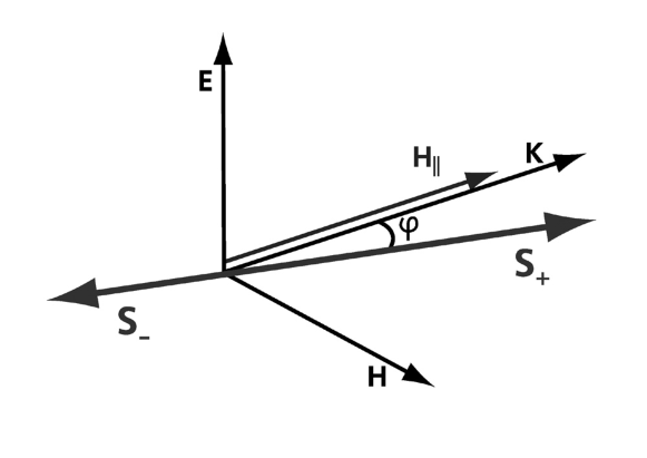
Figure 1: Orientation of the self-polarization axis for the Redmond field.

The above formulas are illustrated by Figure 1. In the Redmond field one has ${\bf t}_{0}=g{\bf n},$ hence the self-polarization axis precesses about wave vector of electromagnetic wave by the angle

$$\tan\varphi=\frac{g|d|}{1+2g\mu_{0}H_{\parallel}/\omega(nu)}.$$ (59)

If the condition $\sin\varphi<|d|$ is valid, self-polarization is total, hence the particle only scatters the external wave. If $\sin\varphi>|d|$ radiative transitions between states with positive and negative projections on this axis exist, frequencies of transitions being different.

It must be emphasized that the formulas for the probability of the radiative transition and radiation power are based on the solutions of equation (5). Obviously, the above deductions will be also true if we replace tensor $H^{\mu\nu}$ by any antisymmetric tensor. In [28] the spin evolution equation was deduced for a neutrino, — a particle involved in weak interaction. This equation possesses the same structure as BMT equation, it can be obtained by the substitution of the electromagnetic field tensor $F_{\mu\nu}$ in the following way:

$$F_{\mu\nu}\rightarrow E_{\mu\nu}=F_{\mu\nu}+G_{\mu\nu}.$$ (60)

The tensor $G_{\mu\nu}$ describes the coherent interaction of neutrino with moving and polarized matter. In the general case of neutrino interacting with background fermions $f$ we have

$$G^{\mu\nu}=\epsilon^{\mu\nu\rho\lambda}g^{(1)}_{\rho}u_{\lambda}-(g^{(2)\mu}u^{\nu}-u^{\mu}g^{(2)\nu}).$$ (61)

Here

$$g^{(1)\mu}=\sum_{f}\rho^{(1)}_{f}j_{f}^{\mu}+\rho^{(2)}_{f}\lambda_{f}^{\mu},\ \ g^{(2)\mu}=\sum_{f}\xi^{(1)}_{f}j_{f}^{\mu}+\xi^{(2)}_{f}\lambda_{f}^{\mu},$$ (62)

where $j_{f}^{\mu}$ are fermion currents and $\lambda^{\mu}_{f}$ are fermion polarizations (summation is performed over all fermions $f$ of the background). The explicit expressions for the coefficients $\rho_{f}^{(1),(2)}$ and $\xi_{f}^{(1),(2)}$ could be found if a special model of neutrino interaction is chosen.

So if, in equation (5), we replace $H^{\mu\nu}$ by the tensor $Z^{\mu\nu}=-{\raise 3.01385pt\hbox{${\scriptstyle 1}$}\!\mathord{\left/{\vphantom{{1}{2}}}\right.\kern-1.2pt}\!\lower 3.01385pt\hbox{${\scriptstyle 2}$}}e^{\mu\nu\rho\lambda}E_{\rho\lambda}$, solutions of such equation may be used for determining the intensity of neutrino spin light in matter and the probability of neutrino radiative transition. Just this method was used in [29, 30] for calculating characteristics of spin light within the quasi-classical approximation. If the matter density is assumed to be constant, which implies that $Z^{\mu\nu}$ is coordinate independent, it is possible to obtain the formulas for processes in matter and external constant electromagnetic fields, for example, in magnetized plasma. The results can be found by the substitution

$$H^{\mu}\rightarrow Z^{\mu}=H^{\mu}+\mu_{0}\big{(}{g}^{(1)\mu}-u^{\mu}({g}^{(1)}u)\big{)}$$ (63)

in equations (45) – (48), obtained for the radiation in a magnetic field.

It should be emphasized that the results obtained in this section agree in the quasi-classical region with those obtained by the methods of quantum electrodynamics in the cases when such calculations were carried out [1, 2, 3, 4, 5, 6, 31].

It is of interest to compare the orders of magnitude of the radiation power $I$ of a neutral particle and the classical radiation power of a charged particle $I_{0}$ (see, for instance, [12]). If these particles have close values of mass, e.g., a proton and a neutron, it is easy to find that

$$\frac{I}{I_{0}}\sim\left\{\left(\frac{H_{0}}{H_{cr}}\right)^{2},\left(\frac{\hbar\dot{H}_{0}}{mc^{2}H_{0}}\right)^{2}\right\},$$ (64)

where the notations are the same as in eq. (2).

Therefore, the radiation powers of a charged particle and that of a neutral particle have the same orders of magnitude either in superstrong fields, which can exist in the vicinity of astrophysical objects of pulsar type, or in very high-frequency fields.

5 Conclusions

Two important conclusions follow from the obtained results. First of all, neutral particles can emit radiation without spin flip. This possibility depends on the following circumstance. Particle polarization is well defined in the rest frame. To determine polarization in the laboratory frame it is necessary to make Lorentz transformation along the kinetic momentum of the particle. However, for the particle in an external field, directions of kinetic and canonical momenta, generally speaking, are different. That is why radiative transitions without spin flip do not contradict conservation laws. Therefore commonly used description of radiative transitions of neutral particles as transitions with spin flip is perfectly true only when transitions from the state which is opposite to the total self-polarization state are considered.

As a result of radiative transition, the particle always goes to the state with the spin parallel to the self-polarization axis. So even for the process in homogeneous magnetic field, the transition probability divides into transition probabilities with and without spin flip. When the particle moves in inhomogeneous, or especially in non-stationary electromagnetic field, the radiative transition without spin flip occurs even from the total self-polarization state. For example, this effect is inherent in the process in the plane-wave field. In this case the particle taken in the state of total polarization emits radiation with the frequency of the external wave (i. e. it scatters the external wave).

In the second place, there are configurations of external fields for which total polarization states of the particles do not exist. The example of such configuration is the Redmond field.

References

References

• [1] Ternov I M, Bagrov V G and Khapaev A M 1965 Sov. Phys. JETP 21 613 (Zh. Eksp. Teor. Fiz. 48 921).
• [2] Ternov I M, Bagrov V G, Kruzhkov V M and Khapaev A M 1967 Izv. Vyssh. Uchebn. Zaved., Fiz. 10(4) 30.
• [3] Skobelev V V 1989 Sov. Phys. JETP 68 221 (Zh. Eksp. Teor. Fiz. 95 391).
• [4] Ternov I M, Bagrov V G, Bordovitsyn V A and Markin Ju A 1967 Sov. Phys. JETP 25 1054 (Zh. Eksp. Teor. Fiz. 52 1584).
• [5] Vshivtsev A S, Potapov R A and Ternov I M 1994 J. Exp. Theor. Phys. 78 593 (Zh. Eksp. Teor. Fiz. 105 1108).
• [6] Ternov I M, Bagrov V G and Khalilov V R 1969 Vestn. MGU. Fiz. Astr. 10(2) 113.
• [7] Bagrov V G, Bozrikov V V, Gitman D M, et al. 1974 Izv. Vyssh. Uchebn. Zaved., Fiz. 17(6), 150. Bagrov V G, Bozrikov V V, Gitman D M, et al. 1974 Izv. Vyssh. Uchebn. Zaved., Fiz. 17(7), 138.
• [8] Bagrov V G and Stepanov V E 1967 Izv. Vyssh. Uchebn. Zaved., Fiz. 10(6) 142.
• [9] Bordovitsyn V A and Gushchina V S 1994 Russ. Phys. J. 37 49 8(Izv. Vyssh. Uchebn. Zaved., Fiz. 37(1) 53). Bordovitsyn V A and Gushchina V S 1995 Russ. Phys. J. 38 155 (Izv. Vyssh. Uchebn. Zaved., Fiz. 38(2) 63). Bordovitsyn V A and Gushchina V S 1995 Russ. Phys. J. 38 293 (Izv. Vyssh. Uchebn. Zaved., Fiz. 38(3) 83).
• [10] Bordovitsyn V A 1993 Russ. Phys. J. 36 1046 (Izv. Vyssh. Uchebn. Zaved., Fiz. 36(11) 39).
• [11] Bordovitsyn V A and Gushchina V S 1998 in Synchrotron Radiation Theory and its Development, edited by V. A. Bordovitsyn, Series on Synchrotron Radiation Technique and Applications – Vol. 5 (World Scientific, Singapore, 1998), pp. 179-235.
• [12] Sokolov A A, Ternov I M, Zhukovsky V Ch and Borisov A V 1988 Quantum electrodynamics (Moscow: Mir).
• [13] Lobanov A E and Pavlova O S 2000 Phys. Lett. A 275 1.
• [14] Lobanov A E and Pavlova O S 2000 Moscow Univ. Phys. Bull. 55(2) 19, (Vestn. MGU. Fiz. Astr. 41(2) 18). Lobanov A E and Pavlova O S 2000 Moscow Univ. Phys. Bull. 55(4) 72, (Vestn. MGU. Fiz. Astr. 41(4) 62).
• [15] Bargmann V, Michel L and Telegdi V 1959 Phys. Rev. Lett. 2 435.
• [16] Ternov I M, Khalilov V R and Pavlova O.S. 1978 Sov. Phys. J. 21 1593 (Izv. Vyssh. Uchebn. Zaved., Fiz. 21(12) 89). Ternov I M, Khalilov V R and Pavlova O.S. 1979 Sov. Phys. J. 22 1400 (Izv. Vyssh. Uchebn. Zaved., Fiz. 22(2) 39).
• [17] Ternov I M 1997 Introduction to Physics of Spin of Relativistic Particles [in Russian] (Moscow: Moscow State Univ. Press).
• [18] Lobanov A E 2003 hep-ph/0311021.
• [19] Lobanov A E and Pavlova O S 1999 Moscow Univ. Phys. Bull. 54(4) 1 (Vestn. MGU. Fiz. Astr. 40(4) 3).
• [20] Brichkov Yu A and Prudnikov A P 1977 Generalized integral transformations [in Russian] (Moscow: Nauka).
• [21] Sokolov A A and Ternov I M 1968 Synchrotron radiation (Berlin: Akademie-Verlag, N.Y.: Pergamon Press).
• [22] Lobanov A E, Pavlova O S and Chizhov G A 2002 Moscow Univ. Phys. Bull. 57(4) 65 (Vestn. MGU. Fiz. Astr. 43(4) 60).
• [23] Lobanov A E 1997 Moscow Univ. Phys. Bull. 52(2) 85 (Vestn. MGU. Fiz. Astr. 38(2) 59).
• [24] Bogolubov N N, Logunov A A, Oksak A I and Todorov I T 1987 General Principles of Quantum Field Theory [in Russian] (Moscow: Nauka); Engish transl., Kluwer, Dordrecht (1990).
• [25] Bordovitsyn V A, Ternov I M and Bagrov V G 1995 Physics – Uspekhi 38 1037 (Uspekhi Fiz.Nauk 165 1084).
• [26] Jackson J D 1976 Rev. Mod. Phys. 48 417.
• [27] Bagrov V G, Belov V V and Trifonov A Ju 1993 J. Phys. A: Math. Gen. 26 6431.
• [28] Lobanov A E and Studenikin A I 2001 Phys. Lett. B 515 94.
• [29] Lobanov A E and Studenikin A I 2003 Phys. Lett. B 564 27.
• [30] Lobanov A E and Studenikin A I 2004 Phys. Lett. B 601 171.
• [31] Lobanov A E 2005 Phys. Lett. B 619 136.