Integral and derivative dispersion relations, analysis of the forward scattering data.

Abstract

Integral and derivative dispersion relations (DR) are considered for the forward scattering $pp$ and $\bar{p}p$ amplitudes. A new representation for the derivative DR, valid not only at high energy, is obtained. The data on the total cross sections for $pp(\bar{p}p)$ interaction as well as the data on the parameter $\rho$ are analyzed within the various forms of the DR and high-energy Regge models. It is shown that three models for the Pomeron, Simple pole Pomeron, Tripole Pomeron and Dipole Pomeron (the both with the intercept equal unit) lead to practically equivalent description of the data at $\sqrt{s}>$5 GeV. It is also shown that the correctly calculated low-energy part of the dispersion integral (from the two-proton threshold up to $\sqrt{s}=$5 GeV) allows to reproduce well the $\rho$ data at low energies without additional free parameters.

1 Introduction

The energy dependence of the hadronic total cross sections as well as that of the parameters $\rho=\Re eA(s,0)/\Im mA(s,0)$ - the ratios of the real to the imaginary part of the forward scattering amplitudes - was widely discussed quite a long time ago (see rhohist ; DDR and references therein). However, in spite of recent detailed investigations on the subject COMPETE , the theoretical situation remains somewhat undecided, mainly because of the $\rho$ parameter.

In the papers COMPETE , all available data on $\sigma_{tot}(s)$ and $\rho(s)$ for hadron-hadron, photon-hadron and photon-photon interactions were considered. Many analytical models for the forward scattering amplitudes were fitted and compared. The ratio $\rho$ was calculated in explicit form, from the imaginary part parametrised by contributions from the pomeron and secondary reggeons. The values of the free parameters were determined from the fit to the data at $s\geq s_{min}$, where $\sqrt{s_{min}}=5$ GeV. Omitting all details, we note here the main two conclusions. The best description of the data is obtained for the model with $\sigma_{tot}$ rising as $\log^{2}s$. The model with $\sigma_{tot}(s)\propto s^{\epsilon},\epsilon>0$ was excluded from the list of the best models (in accordance with COMPETE criteria, see details in COMPETE ).

Analysis of these results shows that they are due to a poor description of $\rho$ data at low energy. On the other hand, there are a few questions concerning the explicit Regge-type models usually used for the analysis and description of the data. How low in energy can the Regge parametrisations be extended, as they are written as functions of the asymptotic variable $s$ rather than the “Regge” variable $\cos\theta_{t}$ ($=E/m$ in the laboratory system for identical colliding particles)? At which energies can the “asymptotic” normalization

$$\sigma_{tot}(s)=(1/s)\Im mA(s,0)$$ (1)

instead of the standard one

$$\sigma_{tot}(s)=(1/2mE)\Im mA(s,0)$$ (2)

be used? And last, how much do the analytic expressions for $\rho$ based on the derivative dispersion relations deviate from those calculated in the integral form?

In this paper, we try to answer these questions considering three pomeron models for $pp$ and $\bar{p}p$ interactions at $\sqrt{s}\geq 5$ GeV.

2 Integral and derivative dispersion relations.

Assuming, in accordance with many analyzes, that the odderon does not contribute asymptotically at $t=0$, one can show that the integral dispersion relations (IDR) for $pp$ and $\bar{p}p$ amplitudes can be reduced to those with one subtraction constant rhohist :

$$\begin{array}[]{lll}\rho_{\pm}\sigma_{\pm}&=&\frac{B}{2m_{p}p}\,\,+\\ &+&\frac{E}{\pi p}\,{\rm P}\!\int\limits_{m_{p}}^{\infty}\left[\frac{\sigma_{\pm}}{E^{\prime}(E^{\prime}-E)}-\frac{\sigma_{\mp}}{E^{\prime}(E^{\prime}+E)}\right]p^{\prime}\,dE^{\prime}\end{array}$$ (3)

where $m_{p}$ is the proton mass, $E$ and $p$ are the energy and momentum of the proton in the laboratory system, and $B$ is a subtraction constant, usually determined from the fit to the data. The indices $+(-)$ stand respectively for the $pp$ and $(\bar{p}p)$ amplitudes. The standard normalization (2) is chosen in Eq.(3).

In the above expression, the contributions of the integral over the unphysical cuts from the two-pion to the two-proton threshold are omitted because they are $\lesssim 1\%$ (see, e.g. valeng ) in the region of interest ($\sqrt{s}\geq 5$ GeV).

The derivative dispersion relations (DDR) were obtained DDR separately for crossing-even and crossing-odd amplitudes

$$f_{\pm}(s,0)=A_{+}(s,0)\pm A_{-}(s,0).$$ (4)

They are very useful in a practice due to their simple analytical form at high energies, $E\gg m_{p}$:

$$\Re ef_{+}(E,0)\approx E\tan\left[\frac{\pi}{2}E\frac{d}{dE}\right]\Im mf_{+}(E,0)/E.$$ (5)

However it is important to estimate the corrections to these asymptotic relations (5) if one is to use them at finite $s$.

It will be shown in the forthcoming paper that one can obtain for the even part of amplitude

$$\begin{array}[]{lll}\Re ef_{+}(E,0)&=&B_{+}+E\tan\left[\frac{\pi}{2}E\frac{d}{dE}\right]\Im mf_{+}(E,0)/E\,-\\ &-&\frac{2}{\pi}\sum\limits_{p=0}^{\infty}\frac{C_{+}(p)}{2p+1}\left(\frac{m_{p}}{E}\right)^{2p}\end{array}$$ (6)

with

$$C_{+}(p)=\frac{e^{-\xi D_{\xi}}}{2p+1+D_{\xi}}[\Im mf_{+}(E,0)-E\Im mf^{\prime}_{+}(E,0)].$$

where $f^{\prime}=df/dE$ and $D_{\xi}=d/d\xi,\xi=\ln(E/m_{p})$.

It can be proven, using the properties of $\exp(-\xi D_{\xi}),$ that $C_{+}(p)$ does not depend on $E$. A similar expression is obtained for the crossing-odd part of the amplitudes.

3 Phenomenology.

Our aim is to compare the fits of three pomeron models with $\rho(s)$ calculated by two methods: the integral dispersion relation, and the asymptotic form of the DDR but with a subtraction constant.

We apply as a first step the IDR and DDR only to $pp$ and $\bar{p}p$ data, fitting the high-energy models to the data at $\sqrt{s}\geq 5$ GeV.

3.1 Low-energy data.

Low-energy total cross sections for $pp$ (143 points) and $\bar{p}p$ (220 points) interactions at $\sqrt{s}<5$ GeV are explicitly parameterized and the values of the free parameters are determined from a fit to the data at $s<s_{min}$ (all data on $\sigma$ and $\rho$ are taken from data ). Thus we perform an overall fit in three steps.

1. The chosen model for high-energy cross-sections is fitted to the data on the cross sections only at $s>s_{min}$.

2. The obtained “high-energy” parameters are fixed. The “low-energy” parameters are determined from the fit at $s<s_{min}$, but with $\sigma_{pp}^{\bar{p}p}(s_{min})$ given by the first step.

3. The subtraction constant $B_{+}$ is determined from the fit at $s>s_{min}$ with all other parameters kept fixed.

Then, without fitting, we calculate the ratios $\rho_{pp}$ and $\rho_{\bar{p}p}$ at all energies above the physical threshold.

3.2 High energy. Pomeron models.

We consider three models leading to different asymptotic behaviors for the total cross sections. We start from the explicit parameterization of the total $pp$ and $\bar{p}p$ cross-sections, then, to find the ratios of the real to imaginary parts, we apply the IDR making use of the second method for a calculation of the low-energy part of the dispersion integral. Then we compare results for ratios calculated through the DDR.

All the models include the contributions of pomeron, $f$ and $\omega$ reggeons (we consider these reggeons as effective ones because it is not reasonable to add other secondary reggeons provided only the $pp$ and $\bar{p}p$ data are fitted.)

$$\sigma_{pp}^{\bar{p}p}={\cal P}(E)+R_{f}(E)\pm R_{\omega}(E),$$ (7)

where $R_{f}=R_{+},R_{\omega}=R_{-}$ and

$$R_{\pm}(E)=g_{\pm}\left(E/\lambda m_{p}\right)^{\alpha_{\pm}(0)-1}.$$ (8)

The parameter $\lambda$ can play a role only for the pomeron term in the triple pole model (see below), in the simple pole and dipole models $\lambda=1$.

When the imaginary part of amplitude is integrated in IDR we consider (for comparison) two kinds of normalization: the standard one defined in Eq. (2) and the asymptotic one given by Eq. (1). For the latter case, in the expressions for cross-sections, the replacement $E/\lambda m_{p}\to s/s_{1}$ is made.

Besides, we compare our results with the models which are written as functions of $-is$ and with the asymptotic normalization (1).

$$\begin{array}[]{lll}\frac{1}{s}A^{\bar{p}p}_{pp}(s,0)&=&i{\cal P}(-is)+iR_{f}(-is)\pm R_{\omega}(-is)\end{array}$$ (9)

We denote such fits as “$-is$ fits”. We present the results of the fits using DDR (with a subtraction constant) and of standard fits with amplitudes defined in accordance with “$-is$” rule.

Simple pole pomeron model (SP). In this model, the intercept of the pomeron is larger than unity d-l

$${\cal P}(E)=g\left(E/(\lambda m_{p})\right)^{\alpha_{\cal P}(0)-1}.$$ (10)

Dipole pomeron model (DP). The pomeron in this model is a double pole in the complex angular momentum plane with intercept $\alpha_{{\cal P}}(0)=1$.

$${\cal P}(E)=g_{1}+g_{2}\ln(E/\lambda m_{p}).$$ (11)

Tripole pomeron model (TP) The pomeron is the hardest complex $j$-plane singularity allowed by unitarity: the triple pole at $t=0$ and $j=1$.

$${\cal P}(E)=g_{1}+g_{2}\ln^{2}(E/\lambda m_{p}).$$ (12)

4 Results, discussion and conclusions.

The quality of the fits is presented in the Table, where $\chi^{2}$ per number of experimental points is shown. In the Figures we show the curves only for the simple-pole pomeron model. For other models the curves are practically the same in the region where data are available.

	Standard		Asymptotic
	normalization		normalization
	IDR	DDR	IDR	$"-is",B=0$
Simple Pole	1.046	1.065	1.112	1.121
Double Pole	1.053	1.045	1.132	1.079
Triple Pole	1.044	1.046	1.111	1.115

Table. The values of the $\chi^{2}$ per point ($\chi^{2}/N_{p}$) obtained in the various pomeron models and through the different methods for the calculation of the ratio $\rho$. Both $\sigma_{tot}$ and $\rho$ are included.

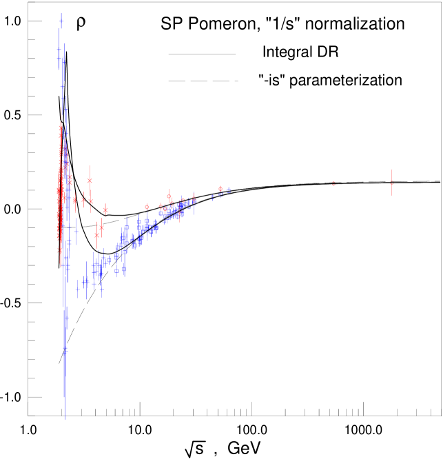
Figure 1: The IDR fit with asymptotic normalization and the “$-is$” fit.

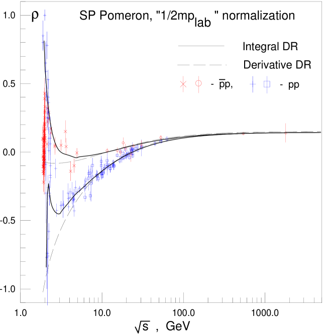
Figure 2: The integral and derivative dispersion relation fit with the standard normalization (see text for details).

As one can see from the Table, all models give similar descriptions of the data on $\sigma_{tot}$ and $\rho$. Evidently, the fit with the integral dispersion relations and with the standard normalization is preferable. While the data on $\sigma$ are described with $\chi^{2}/N_{p}\approx 0.91$, the data on $\rho$ are described less well, with a $\chi^{2}/N_{p}\approx 1.5$ in $pp$ case. We believe that this occurs because of the bad quality of the $\rho$ data.

We would like to note that the values of $\rho$ calculated using DDR deviate from those calculated with IDR even at $\sqrt{s}\lesssim 7-8$ GeV (see Fig. 2). It means that in order to have more correct values of the $\rho$ at such energies, one must use the IDR rather than explicit analytical expressions from the DDR.

The neglect of the subtraction constant, together with the use of asymptotic formulae in a non-asymptotic domain, may be the source of the conclusion of COMPETE excluding the simple-pole model from the list of the best models. Inclusion of these (non-asymptotic) terms improves the description of $\rho$ considerably, and may lead to different conclusions regarding the simple-pole model.

However, in order to have these final conclusions, one will have to make a complete (a la COMPETE) analysis of the all data, including cross sections and $\rho$ for $\pi p$ and $Kp$ interactions.

References

- (1) M.L. Goldberger, Y.Nambu, R. Oehme, Ann. Phys. 2 (1957) 226; P. Söding, Phys. Lett. 8 (1964) 285; M.M. Block, R.N. Cahn, Rev. Mod. Phys. 57 (1985) 563; U. Amaldi et al., Phys. Lett. B66 (1977) 390; P. Kroll, Schwenger W., Nucl. Phys. A503 (1989) 865; C. Auger et al. (UA4 Collab.), Phys. Lett. B315 (1993) 503; P. Desgrolard, M. Giffon, E.S. Martynov, Nuovo Cimento 110A (1997) 537.
- (2) V.N. Gribov, A.A. Migdal, Yad. Fiz. 8 (1968) 1002; J.B. Bronzan, G.L. Kane, U.P. Sukhatme, Phys. Lett. B49 (1974) 276; K. Kang, B. Nicolescu, Phys. Rev. D11 (1975) 2461.
- (3) J.R. Cudell et al. (COMPETE Collab.), Phys. Rev. D65 (2002) 074024; Phys. Rev. Lett. 89 (2002) 201801.
- (4) A.I. Lengyel, V.I. Lengyel, Yad. Fiz. 11 (1970) 669.
- (5) A. Donnachie, P.V. Landshoff, Phys. Lett. B296 (1992) 227.
- (6) http://wwwppds.ihep.su:8001/hadron.html
- (7) J.R. Cudell, A. Lengyel, E. Martynov, O.V. Selyugin, hep-ph/0310198.