Vector Meson Photoproduction from the BFKL Equation II: Phenomenology

Abstract:

Diffractive vector meson photoproduction accompanied by proton dissociation is studied for large momentum transfer. The process is described by the non-forward BFKL equation which we use to compare to data collected at the HERA collider.

1 Introduction

In a previous paper, [1], we performed a detailed theoretical study of the diffractive production of vector mesons at high momentum transfer in $\gamma p$ collisions. We worked throughout in the leading logarithmic BFKL framework [2] and factorised the meson production from the hard subprocess using a set of meson light-cone wavefunctions.

The process is illustrated in Figure 1. The photon and proton collide to produce a final state containing a vector meson and the products of a proton dissociation. The meson is produced with large transverse momentum, the square of which is equal to the Mandelstam variable $-t$, and this is in turn much smaller than the available centre-of-mass energy $s$, i.e. $s\gg-t\gg\Lambda_{\mathrm{QCD}}^{2}.$ This hierarchy ensures that the meson and the proton dissociation are far apart in rapidity. Note, since we will always integrate over the products of the proton dissociation we do not exclude the possibility that the proton may scatter elastically. However, this contribution is negligibly small for sufficiently large $t$ whence the finally state is dominated by configurations containing a single jet with transverse momentum balancing that of the meson [3].

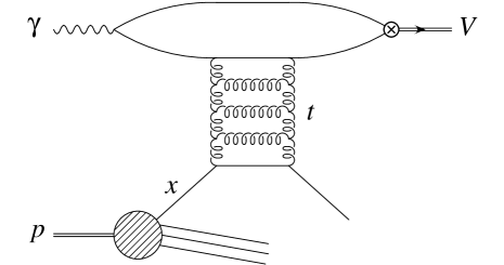
Figure 1: Diffractive vector meson photoproduction at large momentum transfer.

This process has been subject to considerable experimental investigation in recent years, with the measurement of the $t$-distribution of the meson ($\rho$, $\phi$ and $J/\Psi$) [4, 5] and the spin-density matrix elements extracted from its decay [4, 5] being the highlights. It is the purpose of this paper to compare the theoretical results of [1] to the data. Before doing so, we recall the status of diffractive meson production at high-$t$ prior to this analysis.

The experimental data indicate that the cross-section $d\sigma/dt\sim 1/t^{3}$ for $\rho$ and $\phi$ production. Moreover, the relative smallness of the $r^{04}_{00}$ spin-density matrix element suggests that the interactions tend to produce transversely polarised mesons. This is in stark contrast with simple theoretical expectations. Lowest order perturbative QCD does indeed predict a $\sim 1/t^{3}$ distribution but for longitudinally polarised mesons. For transversely polarised mesons, the expected distribution is $\sim 1/t^{4}$. This observation has led the authors of [6] to postulate that the production of transverse mesons is enhanced by the presence of a large non-perturbative coupling of the photon to chiral odd quark-antiquark configurations. The authors of [6] also identified the breakdown of perturbative factorisation in the two-gluon exchange model due to divergent contributions from configurations where either the quark or antiquark carry all the momentum of the meson (i.e. end-point contributions). They argued that this divergent behaviour would be tamed by Sudakov effects and that the dominant chiral odd amplitude was in any case free of problems. In contrast, the authors of [7] make a qualitative argument that it is precisely these end-point contributions which are responsible for the $1/t^{3}$ behaviour seen in data rather than the $1/t^{4}$ which would be expected in perturbation theory. Finally, we should also comment on the apparently naive approach of [8]. In this analysis, longitudinal meson production is suppressed by virtue of the fact that the quark and antiquark share equally the longitudinal momentum of the meson, and transverse meson production is enhanced due to the use of the constituent quark mass. Consequently, in what follows we shall take care to comment on each of the above analyses as appropriate and we shall pay particularly close attention to the end-point behaviour; there being no end-point divergences in the BFKL treatment, even for massless quarks.

Before proceeding we should summarise the experimental analyses. The ZEUS data are for the energy range 80 GeV$<W_{\gamma p}<100\,\text{GeV}$ with the mean value approximately central. Their measurements are for 1 GeV${}^{2}<-t<10$ GeV² and they make the cut $-(M_{X}^{2}-m_{p}^{2})/t<100$ where $M_{X}$ is the mass of the proton dissociation products and $m_{p}$ is the mass of the proton. The relation

$$M_{X}^{2}-m_{p}^{2}=-t(1/x-1)$$ (1)

translates this to a cut of $x>0.01$ where $x$ is the longitudinal momentum fraction of the struck parton. ZEUS quotes a photon virtuality $Q^{2}<0.02\,\text{GeV}^{2}$ with $\langle Q^{2}\rangle\sim 10^{-5}\,\text{GeV}^{2}$. This allows us to neglect $Q^{2}$ in the kinematic relations and in our theoretical calculation.

The H1 data are for $J/\psi$ production, and in the energy range 50 GeV $<W_{\gamma p}<150\,\text{GeV}$ with the mean value approximately central. Their measurements are for 2 GeV${}^{2}<-t<30\,\text{GeV}^{2}$ and they cut in the ‘elasticity’ variable $z_{e}$, which is related to $M_{X}$ to a good approximation (for the $J/\psi$) by

$$z_{e}\simeq 1-(M_{X}^{2}-t)/W_{\gamma p}^{2}.$$ (2)

H1 quote $M_{X}<30\,\text{GeV}$ which translates to $z_{e}>0.95$ and $x>-t/(1-z_{e})s$. The photon virtuality is restricted to satisfy $Q^{2}<1\,\text{GeV}^{2}$ with $\langle Q^{2}\rangle\sim 0.06\,\text{GeV}^{2}$, again small enough to regard the photon as being real.

Following [3], we write the cross-section as a product of the parton level cross-section and parton distribution functions:

$$\frac{d\sigma(\gamma p\rightarrow VX)}{dt\,dx}\;=\;\biggl{(}\frac{4N_{c}^{4}}{(N_{c}^{2}-1)^{2}}G(x,t)+\sum_{f}[q_{f}(x,t)+\bar{q}_{f}(x,t)]\biggr{)}\;\frac{d\sigma(\gamma q\rightarrow Vq)}{dt},$$ (3)

where $N_{c}=3$, $G(x,t)$ and $q_{f}(x,t)$ are the gluon and quark distribution functions respectively and $s$ is the $\gamma p$ centre-of-mass energy squared. The struck parton in the proton, that initiates a jet in the proton hemisphere, carries a fraction $x$ of the longitudinal momentum of the incoming proton.

The parton level cross-section, characterised by the invariant collision energy squared $\hat{s}=xs$, is expressed in terms of the helicity amplitudes $M_{\lambda\lambda^{\prime}}(\hat{s},t)$ ($\lambda$ is the photon helicity and $\lambda^{\prime}$ is the meson helicity):

$$\frac{d\sigma}{dt}=\frac{1}{16\pi\hat{s}^{2}}\left(|M_{++}(\hat{s},t)|^{2}+|M_{+0}(\hat{s},t)|^{2}+|M_{+-}(\hat{s},t)|^{2}\right)$$ (4)

The experimenters also measure the spin density matrix elements $r^{04}_{ij}$ which are extracted from the angular distribution of the decay products of the vector meson:

$$\frac{d^{2}\sigma}{d\cos\theta_{h}\,d\phi_{h}}\propto\biggl{[}\frac{1}{2}(1\mp r^{04}_{00})\pm\frac{1}{2}(3r^{04}_{00}-1)\cos^{2}\theta_{h}$$

$$\mp\sqrt{2}\text{Re}[r^{04}_{00}]\,\sin 2\theta_{h}\,\cos\phi_{h}\mp r^{04}_{1-1}\,\sin^{2}\theta_{h}\,\cos 2\phi_{h}\biggr{]},$$ (5)

where the upper (lower) signs are for spin-0 (spin-1/2) particles. $\theta_{h}$ and $\phi_{h}$ are the spherical polar angles of the positive particle of the two body decay of the meson, where the vector meson momentum defines the $z$-axis and the $x$-axis (which fixes $\phi_{h}=0$) is defined to lie in the direction of the hard momentum transfer, ${\bf q}$. Note that $|{\bf q}|^{2}=-t$ in what follows. The $r$-matrix elements can be written [9, 10, 11]

$$r^{04}_{00}={\langle|M_{+0}|^{2}\rangle\over\langle|M_{++}|^{2}+|M_{+0}|^{2}+|M_{+-}|^{2}\rangle},$$ (6)

$$r^{04}_{10}={1\over 2}{\langle M_{++}M^{*}_{+0}+M_{+-}M^{*}_{-0}\rangle\over\langle|M_{++}|^{2}+|M_{+0}|^{2}+|M_{+-}|^{2}\rangle},$$ (7)

$$r^{04}_{1-1}=\frac{1}{2}{\langle M_{++}M_{+-}^{*}+M_{+-}M_{++}^{*}\rangle\over\langle|M_{++}|^{2}+|M_{+0}|^{2}+|M_{+-}|^{2}\rangle},$$ (8)

where $\langle...\rangle$ denotes the integration of the parton level quantities over partonic $x$ with the appropriate cuts. Throughout this paper we choose a fixed value for the $\gamma p$ centre-of-mass energy: $\surd s=W_{\gamma p}=100\,\text{GeV}$.

2 Theoretical Results

We begin by summarising the results of [1] for the relevant matrix elements. We append a superscript to specifiy if the photon-quark coupling is chiral even or chiral odd.

We use the meson distribution amplitudes of [12, 13] and use their notation throughout. The explicit forms for the distribution amplitudes we use can be found in Appendix A. In what follows we systematically include terms of progressively higher twist in the distribution amplitudes in order to ascertain their relative importance. The relevant amplitudes are

$${M}_{+0}^{even}=\frac{isC_{V}f_{V}}{4\sqrt{2}|q|}\int_{0}^{1}du\;(1-2u)\phi_{\|}(u)$$

$$\sum_{n=-\infty}^{n=+\infty}\int_{-\infty}^{\infty}d\nu\frac{\nu^{2}+n^{2}}{[\nu^{2}+(n-1/2)^{2}][\nu^{2}+(n+1/2)^{2}]}\frac{\exp[\chi_{2n}(\nu)z]}{\sin(i\pi\nu)}\,I_{0-1}(\nu,2n,q,u;1),$$

(9)

$${M}_{++}^{even}=\frac{sC_{V}f_{V}M_{V}}{8|q|}\,\int_{0}^{1}du\;\left(\frac{g_{\perp}^{(a)}(u)}{4}-(1-2u)\int_{0}^{u}dv(\phi_{\|}(v)-g_{\perp}^{(v)}(v))\right)$$

$$\times\sum_{n=-\infty}^{n=+\infty}\int_{-\infty}^{\infty}d\nu\frac{\nu^{2}+n^{2}}{[\nu^{2}+(n-1/2)^{2}][\nu^{2}+(n+1/2)^{2}]}\frac{\exp[\chi_{2n}(\nu)z]}{\sin(i\pi\nu)}\,I_{00}(\nu,2n,q,u;1),$$

(10)

$${M}_{+-}^{even}=\frac{sC_{V}f_{V}M_{V}}{8|q|}\int_{0}^{1}du\,\left(\frac{g_{\perp}^{(a)}(u)}{4}+(1-2u)\int_{0}^{u}dv(\phi_{\|}(v)-g_{\perp}^{(v)}(v))\right)$$

$$\times\sum_{n=-\infty}^{n=+\infty}\int_{-\infty}^{\infty}d\nu\frac{\nu^{2}+n^{2}}{[\nu^{2}+(n-1/2)^{2}][\nu^{2}+(n+1/2)^{2}]}\frac{\exp[\chi_{2n}(\nu)z]}{\sin(i\pi\nu)}\,I_{1-1}(\nu,2n,q,u;1).$$

(11)

$${M}_{+0}^{odd}=\frac{isC_{V}f_{V}^{T}M_{V}}{4\sqrt{2}|q|}\int_{0}^{1}du\;\int_{0}^{u}dv(h_{\|}^{(t)}(v)-\phi_{\perp}(v))$$

$$\times\sum_{n=-\infty}^{n=+\infty}\int_{-\infty}^{\infty}d\nu\frac{\nu^{2}+n^{2}}{[\nu^{2}+(n-1/2)^{2}][\nu^{2}+(n+1/2)^{2}]}\frac{\exp[\chi_{2n}(\nu)z]}{\sin(i\pi\nu)}\,I_{{1\over 2}\,-{1\over 2}}(\nu,2n,q,u;0),$$

(12)

$${M}_{++}^{odd}=\frac{sC_{V}f_{V}^{T}}{4|q|}\,\int_{0}^{1}du\;\phi_{\perp}(u)\,$$

$$\times\sum_{n=-\infty}^{n=+\infty}\int_{-\infty}^{\infty}d\nu\frac{\nu^{2}+n^{2}}{[\nu^{2}+(n-1/2)^{2}][\nu^{2}+(n+1/2)^{2}]}\frac{\exp[\chi_{2n}(\nu)z]}{\sin(i\pi\nu)}\,I_{-{1\over 2}\,-{1\over 2}}(\nu,2n,q,u;0),$$

(13)

$${M}_{+-}^{odd}=\frac{sC_{V}f_{V}^{T}M_{V}^{2}}{8|q|}\int_{0}^{1}du\,\int_{0}^{u}dv\int_{0}^{v}d\eta\left(h_{\|}^{(t)}(\eta)-\frac{1}{2}\phi_{\perp}(\eta)-\frac{1}{2}h_{3}(\eta)\right)$$

$$\times\sum_{n=-\infty}^{n=+\infty}\int_{-\infty}^{\infty}d\nu\frac{\nu^{2}+n^{2}}{[\nu^{2}+(n-1/2)^{2}][\nu^{2}+(n+1/2)^{2}]}\frac{\exp[\chi_{2n}(\nu)z]}{\sin(i\pi\nu)}\,I_{{3\over 2}\,-{1\over 2}}(\nu,2n,q,u;0).$$

(14)

where

$$I_{\alpha\beta}(\nu,n,q,u;a) = m\int d^{2}\rho\;\rho^{\alpha+1}\rho^{*\,\beta+1}\,K_{a}(m|\rho|)e^{\frac{i\xi}{4}[q^{*}\rho+q\rho^{*}]}$$ (15)

$$\times [J_{\mu}(q^{*}\rho/4)J_{\tilde{\mu}}(q\rho^{*}/4)-(-1)^{n}\;J_{-\mu}(q^{*}\rho/4)J_{-\tilde{\mu}}(q\rho^{*}/4)],$$

$\xi=2u-1$, $\mu=n/2-i\nu$, $\tilde{\mu}=-n/2-i\nu$, $K_{a}(x)$ is the modified Bessel function and the parameter $a$ equals $1$ for the chiral-even and $0$ for the chiral-odd contributions. In (15) we use complex variable notation for the transverse vectors $\rho$ and $q$, e.g. $\rho=\rho_{x}+i\rho_{y}$.

After some effort [1] one finds

$$I_{\alpha\beta}(\nu,n,q,u;a) = \frac{m}{2}\int^{C^{\prime}+i\infty}_{C^{\prime}-i\infty}\frac{d\zeta}{2\pi i}\Gamma(a/2-\zeta)\Gamma(-a/2-\zeta)\,\tau_{q}^{\zeta}\;(i\,\text{sign}\,(1-2u))^{\alpha-\beta+n}$$ (16)

$$\times \left(\frac{4}{|q|}\right)^{4}\left[\sin\pi(\alpha+\mu+\zeta)\;\right.B(\alpha,\mu,q^{*},u,\zeta)\,B(\beta,\widetilde{\mu},q,u^{*},\zeta)$$

$$- (-1)^{n}\sin\pi(\alpha-\mu+\zeta)\;B(\alpha,-\mu,q^{*},u,\zeta)\,B(\beta,-\widetilde{\mu},q,u^{*},\zeta)\left.\right]$$

where we have introduced the dimensionless parameter $\tau_{q}=4m^{2}/|q|^{2}$ and the conformal blocks

$$B(\alpha,\mu,q^{*},u,\zeta)=(-4u\bar{u})^{-(\mu+2+\alpha+\zeta)/2}\left(\frac{4}{q^{*}}\right)^{\alpha}2^{-\mu}\,\frac{\Gamma(\mu+2+\alpha+\zeta)}{\Gamma(\mu+1)}$$

$$\,{}_{2}F_{1}\left(\frac{\mu+2+\alpha+\zeta}{2}\,,\,\frac{\mu-1-\alpha-\zeta}{2}\,;\,\mu+1\,;\,\frac{1}{4u\bar{u}}\right).$$ (17)

Note, that the sums are performed over even conformal spins $2n$.

We have also introduced the energy variable

$$z=\frac{3\alpha_{s}}{2\pi}\ln\left(\frac{xs}{\Lambda^{2}}\right)$$ (18)

where $\Lambda$ is an undetermined energy scale in the leading logarithmic approximation. The eigenvalues of the BFKL kernel are proportional to

$$\chi_{n}(\nu)\;=\;4\mathcal{R}\mathrm{e}\,\biggl{(}\psi(1)-\psi(1/2+|n|/2+i\nu)\biggr{)}$$ (19)

	$\rho$	$\phi$	$J/\psi$
$Q_{V}$	$1/\sqrt{2}$	$-1/3$	$2/3$

Table 1: The meson electric charge couplings.

and we collect together several factors into $C_{V}$:

$$C_{V}=i\alpha_{s}^{2}\frac{N_{c}^{2}-1}{N_{c}^{2}}eQ_{V}$$ (20)

where $Q_{V}$ is determined by the electric charge of the quarks which make up the meson. The explicit values are listed in Table 1.

All the helicity amplitudes depend upon the vector meson coupling constants; either $f_{V}$ (vector) or $f_{V}^{T}$ (tensor). Table 2 presents the vector and tensor couplings for the relevant mesons. The vector couplings are directly measurable from the electronic decay width of the vector mesons whilst the tensor couplings have been calculated at $\mu=1\,\text{GeV}$ using QCD sum rules [12].

	$\rho$	$\phi$	$J/\psi$
$f_{V}$ [GeV]	$0.216$	$0.231$	0.405
$f_{V}^{T}(1\,\text{GeV})$ [GeV]	$0.160$	$0.215$	(0.405)

Table 2: The meson decay constants [12].

In Table 3 we classify the above set of helicity amplitudes in terms of twist. We work to next-to-leading twist in each amplitude, i.e. we do not consider twist-4 terms in the single and no flip amplitudes.

twist	2	3	4
single-flip	${M}_{+0}^{even}$	${M}_{+0}^{odd}$	$-$
no-flip	${M}_{++}^{odd}$	${M}_{++}^{even}$	$-$
double-flip	$0$	${M}_{+-}^{even}$	${M}_{+-}^{odd}$

Table 3: Classification of the relevant helicity amplitudes in twist.

3 Parameters and prescriptions

Strictly, in perturbation theory, we should use the current quark mass. However, using the current mass renders the chiral odd contribution negligible for light mesons and proves to be incapable of describing the $r$-matrix elements. The authors of [6] noted the importance of introducing a large chiral odd contribution. The method they employ introduces a large non-perturbative coupling of the photon to chiral odd quark-antiquark configurations. We shall take a different approach and replace the current quark mass with the constituent quark mass, i.e. we take $m=m_{V}/2$. We will investigate the sensitivity to this parameter.

We also need to explain how we implement the strong coupling, $\alpha_{s}$ and the scale $\Lambda^{2}$ which appears in (18). We might reasonably expect that $\Lambda^{2}=\beta m_{V}^{2}-\gamma t$ where $\beta$ and $\gamma$ are unknown. To simplify matters, we choose to fix, $\beta=1$ since a change in its value can approximately be traded off with a change in $\alpha_{s}$.

Notice that $\alpha_{s}$ appears in two places. It appears as a prefactor of $\alpha_{s}^{2}$ in every helicity amplitude. It also appears in the definition of $z$ (see (18)). The prefactor arises from the coupling of the two gluons to each impact factor. The coupling in $z$, however, is generated by the gluon couplings inside the gluon ladder. We shall denote these couplings $\alpha_{s}^{IF}$ and $\alpha_{s}^{BFKL}$ respectively. Strictly speaking a fixed value of $\alpha_{s}$ is appropriate to the level of our calculation. However, next-to-leading logarithms cause $\alpha_{s}$ to run. Arguments exist that the effect of these corrections is to effectively fix $\alpha_{s}^{BFKL}$ [14]. Phenomenologically, fixing $\alpha_{s}^{BFKL}$ has proved successful in the past [8, 15] and we will fix it here. We remain free to run or fix the impact factor coupling, $\alpha_{s}^{IF}$, and we shall subsequently make use of this possibility. When we refer to a running coupling in future, we shall be referring to its value at $1\,\text{GeV}$. We note that, as ratios, the $r$-matrix elements are independent of $\alpha_{s}^{IF}$.

In summary, the parameters we shall treat as free for fitting purposes are

$$\alpha_{s}^{IF},\hskip 28.45274pt\alpha_{s}^{BFKL}\hskip 28.45274pt\text{and}\hskip 28.45274pt\Lambda^{2}=m_{V}^{2}-\gamma t.$$ (21)

We shall also show the sensitivity of our variables to the quark mass $m$ though we shall not treat this as a fit parameter.

For other parameters, we shall use either those measured by experiment or estimated in the literature. We shall not vary these. The sensitivity of our predictions to various approximations for the meson distribution amplitudes will be tested by testing the importance of $1/|{\bf q}|^{2}$ suppressed and above terms and by employing three different distribution amplitude prescriptions. We refer to the three prescriptions as the $\delta$-function prescription, the asymptotic distribution amplitude prescription (obtained in the limit $\alpha_{s}\rightarrow 0$) and the full distribution amplitude prescription (of [12, 13]). All necessary information on the meson distribution amplitudes can be found in Appendix A.

4 Phenomenology for the $\rho$ meson

In this section we focus wholly on the phenomenology of the $\rho$ meson. We begin with the most crude approximations for the meson wavefunction and systematically relax these to the point where we eventually treat the meson using the full light-cone wavefunctions of [12, 13].

4.1 The collinear and $\delta$-function approximations

The collinear approximation corresponds to putting the transverse momentum of the quark and antiquark exiting the hard scatter (measured relative to the meson direction) to zero. This approximation generates $\delta$-functions which force the transverse size of the quark-antiquark pair to zero. This fact forces all the higher twist helicity amplitudes to zero so that only ${M}_{+0}^{even}$ and ${M}_{++}^{odd}$ (twist-2) then survive.

The $\delta$-function approximation for the meson distribution amplitudes corresponds to equating

$$\phi_{\|}(u)=\phi_{\perp}(u)=\delta(u-1/2).$$ (22)

The ${M}_{+0}^{even}$ helicity amplitude is zero in this approximation and so the only non-zero amplitude is ${M}_{++}^{odd}$:

$${M}_{++}^{odd}=sC_{V}\frac{8\pi}{t^{2}}\,f_{V}m_{V}\,\hskip 170.71652pt$$

$$\times\sum_{m=-\infty}^{m=\infty}\biggl{(}-\frac{1}{4}\biggr{)}^{|m|}\int\,d\nu\,\frac{\nu^{2}+m^{2}}{(\nu^{2}+(m-1/2)^{2})(\nu^{2}+(m+1/2)^{2})}\;e^{\chi_{m}(\nu)z}\$$

$$\times\int_{-i\infty}^{i\infty}\frac{ds}{2\pi i}\,\tau^{1/2+s+|m|}\,\frac{\Gamma(1-s-i\nu)\,\Gamma(1-s+i\nu)}{\Gamma(1-s/2-i\nu/2)\,\Gamma(1-s/2+i\nu/2)}$$

$$\times\frac{\Gamma^{2}(1/2+s+|m|)}{\Gamma(1/2+s/2-i\nu/2+|m|)\,\Gamma(1/2+s/2+i\nu/2+|m|)}.$$ (23)

Figure 2 shows the predictions for $d\sigma/dt$ for three different sets of parameter values. Running the scale $\Lambda^{2}$ that appears under $s$ in the BFKL logarithm (18) with $t$ or running $\alpha_{s}^{IF}$ with $t$ prove to predict $t$ dependencies that are too steep and incompatible with the data presented by ZEUS [4]. Fixing the strong coupling in the impact factor and in the BFKL ladder in addition to the BFKL logarithm yields a good fit. These results agree with those of [8] for the leading conformal spin component ($n=0$) and [16] for $n>0$.

Since only the ${M}_{++}^{odd}$ amplitude is non-zero with the collinear and $\delta$-function approximations imposed, referring to their definitions ((6), (7), (8)), we see that this enforces all the $r$-matrix elements to zero. Figure 3 shows this prediction in comparison to the ZEUS data. We see that zero $r$-matrix elements are compatible with data for $r^{04}_{00}$, in fair agreement for $r^{04}_{10}$ and in poor agreement for $r^{04}_{1-1}$.

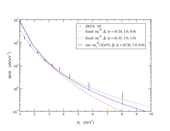
Figure 2: Collinear and $\delta$-function approximation: $d\sigma/dt$ for parameter values, $(\alpha_{s}^{BFKL},\,m)=(0.2,\,m_{\rho}/2)$.

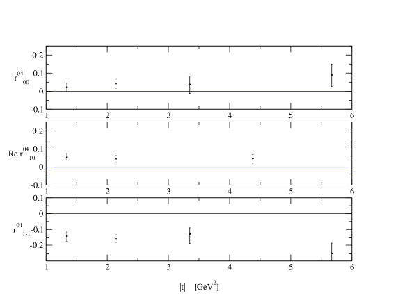
Figure 3: Collinear and $\delta$-function approximation: $r$-matrix elements. The predictions are parameter independent.

4.2 Collinear approximation and asymptotic distribution amplitudes

The use of a $\delta$-function distribution amplitude is a crude approximation. For the charm quark and $J/\psi$ meson, $m_{c}\sim m_{J/\psi}/2$. For this meson, the configurations that provide the dominant contributions should be close to $u\sim 1/2$, i.e. we expect the $\delta$-function approximation to be fair. This is not so for the light $\rho$. The use of the $\delta$-function was motivated purely by past phenomenological success [8]. To understand this success, and to have any hope of predicting the helicity structure of the cross-section, we must relax this crude assumption. For now, we maintain the collinear assumption and use the asymptotic distribution amplitudes. The relevant amplitudes are

$$\phi_{\|}(u)=\phi_{\perp}(u)=6u(1-u).$$ (24)

Now momentum configurations of $u\not=1/2$ contribute and the ${M}_{+0}^{even}$ helicity amplitude is no longer zero.

Figure 4 shows predictions for the cross-section. The ${M}_{+0}^{even}$ amplitude has a less steep $t$ dependence than ${M}_{++}^{odd}$. The higher suppression of the chiral odd term is what we expect since in the definition of the $I_{\alpha\beta}$ integral in ${\bf r}$ space (see (15)), the chiral even amplitudes have a $K_{1}$ function and the chiral odd ones a $K_{0}$. The $r^{04}_{00}$ element is the ratio of the longitudinal component of the cross-section to the total. Figure 5 demonstrates that this longitudinal component is numerically subdominant, but becomes increasingly important with rising $|t|$. The change in the $t$ dependence of the combined cross-section, due to this component, results in the previous fit of $\gamma=0$ and fixed $\alpha_{s}^{IF}$ now being marginal. We now fit the data better by either running $\Lambda^{2}$ with $t$ or $\alpha_{s}^{IF}$ with $t$.

Note that the amplitude ${M}_{+-}$ is still zero in our collinear scheme. This means that the $r^{04}_{1-1}$ $r$-matrix element is still predicted to be zero. As observed for the case of the $\delta$-function distribution amplitude, this is precisely the $r$-matrix most incompatible with such a prediction. Figure 5 shows the effect on the $r$-matrix elements of running the $\Lambda^{2}$ scale with $t$ versus keeping it fixed. We observe that both provide a good fit for $r^{04}_{00}$ and poor predictions for $r^{04}_{10}$ and $r^{04}_{1-1}$. The poor quality of fits to the $r$-matrix elements motivates the progression to higher twist. Higher twist is the only solution to producing a non-zero ${M}_{+-}$ contribution.

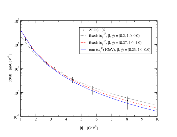
Figure 4: Collinear approximation: $d\sigma/dt$ for parameter values, $(\alpha_{s}^{BFKL},\,m)=(0.2,\,m_{\rho}/2)$.

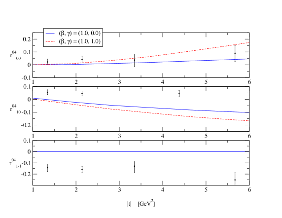
Figure 5: Collinear approximation: $r$-matrix elements for parameter values, $(\alpha_{s}^{BFKL},\,m)$ $=$ $(0.2,\,m_{\rho}/2)$.

4.3 Higher twist effects

Higher twist effects are introduced by relaxing the assumption that a collinear quark and antiquark exit the hard subprocess (i.e. we no longer have dipoles of zero transverse size) or by inclusion of higher Fock states (e.g. $q\bar{q}g$) in the wave function.

Potentially, we must consider the full six helicity amplitudes. The complete set of relevant asymptotic distribution amplitudes are

$$\phi_{\|}(u)=\phi_{\perp}(u)=6u\bar{u}$$

$$g_{\perp}^{(a)}(u)=6u\bar{u}\hskip 28.45274ptg_{\perp}^{(v)}(u)=\frac{3}{4}(1+\xi^{2})$$

$$h_{3}(u)=\frac{3}{2}(1-\xi^{2}),$$ (25)

where $\xi=2u-1$. Substituting these into (9)–(14) we obtain the amplitudes which were presented explicitly in [1]. We do not list them again here.

We want to explore the effect of higher twist terms on our observables by systematically adding suppressed terms. Any observable is proportional to products of the helicity amplitudes i.e. ${M}_{ij}{M}^{*}_{kl}$. Consider the (parton level) cross-section for the production of a longitudinal meson:

$$\hskip 42.67912pt\frac{d\sigma_{+0}}{dt}\propto{M}_{+0}{M}^{*}_{+0}=\biggl{(}{M}_{+0}^{even}+{M}_{+0}^{odd}\biggr{)}\biggl{(}{M}_{+0}^{even\,*}+{M}_{+0}^{odd\,*}\biggr{)}$$

$$={M}_{+0}^{even}{M}_{+0}^{even\,*}+{M}_{+0}^{even}{M}_{+0}^{odd\,*}+{M}_{+0}^{odd}{M}_{+0}^{even\,*}+{M}_{+0}^{odd}{M}_{+0}^{odd\,*}$$

$$\hskip 8.5359pt{}^{\text{(twist-2 x twist-2)}}\hskip 8.5359pt{}^{\text{(twist-2 x twist-3)}}\hskip 8.5359pt{}^{\text{(twist-2 x twist-3)}}\hskip 8.5359pt{}^{\text{(twist-3 x twist-3)}}$$

In the expression above we see that the first term is leading (twist-2 x twist-2), the second and third $1/|{\bf q}|$ suppressed (twist-2 x twist-3), and the fourth $1/|{\bf q}|^{2}$ suppressed (twist-3 x twist-3). Note that a (twist-2 x twist-4) term would also be $1/|{\bf q}|^{2}$ suppressed. Next-to-leading power behaviour in observables is therefore the highest level in which we are able to compute. Note that the helicity double-flip amplitude is subleading at this level of approximation as far as the total cross-section is concerned but that it provides the leading behaviour for $r_{1-1}^{04}$.

Figure 6 shows $d\sigma/dt$ for the varying levels of approximation. The effect on the combined cross-section is predominantly that of normalisation. We see that adding in the (twist-2 x twist-3) to the (twist-2 x twist-2) terms has a significant effect, but that adding those next-to-next-to-leading terms that we have knowledge of has much less effect. This reassuring result suggests that the total cross-section is insensitive to the twist-four terms that we have neglected.

Figure 7 shows that the observables $r^{04}_{00}$ and $r^{04}_{10}$ are also relatively insensitive to next-to-next-to leading terms. The $r^{04}_{1-1}$ proves more sensitive. Adding the (twist-3 x twist-3) terms has an effect of order $100\%$. It is not surprising that this observable is the most sensitive to higher twist, since it is zero at leading twist. It therefore appears that we cannot trust our predictions for this $r$-matrix element and that it is not a good observable with which to test the validity of BFKL dynamics. However, Figure 8, makes it clearer what is happening. It shows the ratios of even to odd helicity amplitudes at $x=0.1$. Our twist counting scheme ignores the effect of $|{\bf q}|$-dependent effects in the hard scatter. The plots in Figure 8 are a test of the validity of this assumption. If effects of the hard scatter were the same, we would expect twist counting to give us ${M}_{+0}^{even}/{M}_{+0}^{odd}$ and ${M}_{+-}^{even}/{M}_{+-}^{odd}$ approximately $\propto\sqrt{-t}$ and ${M}_{++}^{even}/{M}_{++}^{odd}$ $\propto 1/\sqrt{-t}$. Our assumption seems reasonable for the $(+0)$ and $(+-)$ amplitudes, however, for $(++)$ the odd and even terms have a similar $t$-dependence. ${M}_{++}^{even}$ is twist-3 but the ${\bf q}$ dependence from the hard scatter boosts its importance to the same significance as the twist-2 pieces. The thick line in the plot of $r^{04}_{1-1}$ in Figure 7, is the prediction where we, in addition to the ${M}_{++}^{odd}{M}_{+-}^{even}$ term, kept the ${M}_{++}^{even}{M}_{+-}^{even}$ term. For $t$ significantly above $1\,\text{GeV}^{2}$, we can see that the effect of terms genuinely $1/|{\bf q}|^{2}$ suppressed and above, is minimal. Thus, though $r_{1-1}^{04}$ is the most sensitive observable to higher twist effects, we can claim to have control over it. We shall therefore, from here on, use the formulae (9)–(14) with the distribution amplitudes computed up to twist-4 for $M_{+-}$ and up to twist-3 for all others. Our control over higher twist suggests that higher twist effects are unlikely to provide the solution to the fact we cannot fit the complete set of $r$-matrix elements.

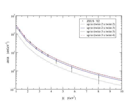
Figure 6: Higher twist effects: $d\sigma/dt$ for parameter values, $(\alpha_{s}^{IF},\alpha_{s}^{BFKL},\,\,\Lambda^{2},\,m)=(0.17,\,0.2,\,m_{V}^{2},\,m_{\rho}/2)$.

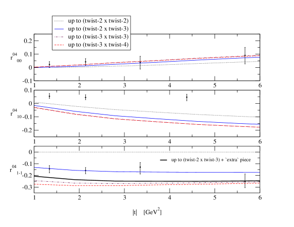
Figure 7: Higher twist effects: $r$-matrix elements for parameter values, $(\alpha_{s}^{BFKL},\,\Lambda^{2},\,m)$ $=$ $(0.2,\,m_{V}^{2},\,m_{\rho}/2)$.

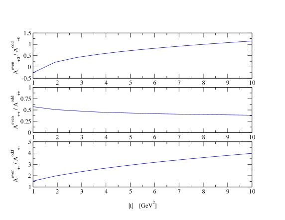
Figure 8: Higher twist effects: even to odd amplitude ratios for parameter values, $(\alpha_{s}^{BFKL},\,\Lambda^{2},\,m)=(0.2,\,m_{V}^{2},\,m_{\rho}/2)$.

4.4 The sensitivity of predictions to parameters

We demonstrated in the previous section that, away from low $t$, our predictions are only weakly sensitive to higher twist corrections. The fit for the $r^{04}_{10}$ $r$-matrix element remained particularly poor, however. In this section we explore the sensitivity of our results to varying the various parameters at our disposal. We shall use a fixed $\alpha_{s}^{IF}=0.17$, and it should then be understood that only the shape of the $t$-distribution matters (its normalisation being adjustable by varying $\alpha_{s}^{IF}$). Of course $\alpha_{s}^{IF}$ cancels in the $r_{ij}^{04}$.

4.4.1 Sensitivity to $\alpha_{s}^{BFKL}$

Figure 9 shows a central curve corresponding to: $(\alpha_{s}^{IF},\,\alpha_{s}^{BFKL},\,\Lambda^{2},\,m)$ $=$
$(0.17,\,0.2,\,m_{\rho}^{2},\,m_{\rho}/2)$. The two other curves show the effect of varying the value of $\alpha_{s}^{BFKL}$ by $25\%$. The effect is primarily that of normalisation.

The $r$-matrix element predictions are shown in Figure 10. $r_{00}^{04}$ is the most sensitive to variations in $\alpha_{s}^{BFKL}$, followed in order by $r_{10}^{04}$ and $r_{1-1}^{04}$. We find $r_{1-1}^{04}$ to be relatively insensitive to this parameter whereas we remind the reader that it proved most sensitive to higher twist. We note that while the general quality of the fits for all the $r$-matrix elements is unaffected by varying $\alpha_{s}^{BFKL}$ by $25\%$, a large value of $\alpha_{s}$ is associated with a larger suppression of the longitudinal cross-section. We also note that the fit to $r^{04}_{10}$ remains poor.

4.4.2 Sensitivity to $\gamma$

The default set, $(\alpha_{s}^{IF},\,\alpha_{s}^{BFKL},\,\Lambda^{2},\,m)=(0.17,\,0.2,\,m_{\rho}^{2},\,m_{\rho}/2)$, that provides the solid curve in Figure 11, is only marginally compatible with the cross-section data. This is because, as previously noted, the longitudinal contribution becomes increasingly important at higher $t$ and this flattens the $t$ dependence. The dotted curve on the same graph demonstrates that we can fit the data much better by running the BFKL scale, $\Lambda^{2}$.

The predictions in Figure 12 for the $r$-matrix elements again show the sign problem in the prediction for $r_{10}^{04}$. Running $\Lambda^{2}$ has not solved this. Note also that the predictions for $r_{00}^{04}$ and $r_{10}^{04}$ are sensitive to the values of the BFKL parameters and in particular, the quality of the fits becomes worse when $\Lambda^{2}$ is run with $t$. We see that when $\Lambda^{2}$ is run, the longitudinal fraction grows quicker than is compatible with data.

4.4.3 Sensitivity to $z$ rapidity

Note that the rapidity variable $z$ increases (or decreases) as we raise $\alpha_{s}^{BFKL}$ (or $\gamma$). It is really this $z$ variable that we have been investigating in the previous subsections. Figure 13 contains a plot for each helicity amplitude at the rapidity values, $z=0.5,\,0.75$ and $1.0$. The number in the brackets in the legends correspond to the areas underneath the curves. Note that the position of the peaks do not shift as we change rapidity. As $z$ decreases all amplitudes fall, but a look at the integrated values demonstrates that the longitudinal amplitudes fall more slowly. If we lower $z$ we raise the ratio of the longitudinal to the transverse contributions.

This observation allows us to play off the effects of varying $\alpha_{s}^{BFKL}$ and $\Lambda^{2}$ simultaneously. A non-zero $\gamma$ value in $\Lambda^{2}$ improves the $t$ dependence of the differential cross-section and in conjunction, increasing $\alpha_{s}^{BFKL}$ drives the longitudinal component down. The fit values $(\alpha_{s}^{IF},\,\alpha_{s}^{BFKL},\,\Lambda^{2})$ $=$ $(0.17,\,0.25,\,m_{\rho}^{2}-t)$ therefore lead to an improved overall fit. The predictions for these values are shown in Figures 14–15. Let us here recall the familiar result that the dependence of all amplitudes on the partonic collision energy $\hat{s}$ is characterised by the BFKL exponent, i.e. $M_{ij}\sim\hat{s}^{\lambda}$ with $\lambda=12\ln 2\,\alpha_{s}^{BFKL}/\pi$, provided that $\hat{s}$ is sufficiently large, say $z>1$.

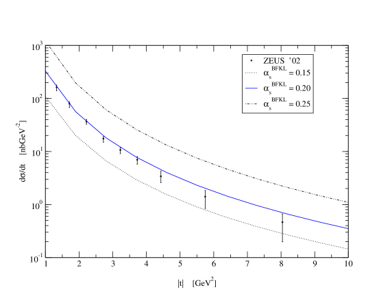
Figure 9: The sensitivity to varying $\alpha_{s}^{BFKL}$: $d\sigma/dt$ for parameter values, $(\alpha_{s}^{IF},\,\Lambda^{2},\,m)$ $=$ $(0.17,\,m_{\rho}^{2}-t,\,m_{\rho}/2)$.

Figure 10: The sensitivity to varying $\alpha_{s}^{BFKL}$: $r$-matrix elements for parameter values, $(\Lambda^{2},\,m)$ $=$ $(m_{\rho}^{2}-t,\,m_{\rho}/2)$.

Figure 11: The sensitivity to varying $\gamma$: $d\sigma/dt$ for parameter values, $(\alpha_{s}^{IF},\,\alpha_{s}^{BFKL},\,m)=(0.17,\,0.2,\,m_{\rho}/2)$.

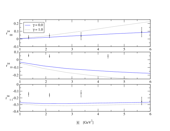
Figure 12: The sensitivity to varying $\gamma$: $r$-matrix elements for parameter values, $(\alpha_{s}^{BFKL},\,m)=(0.2,\,m_{\rho}/2)$.

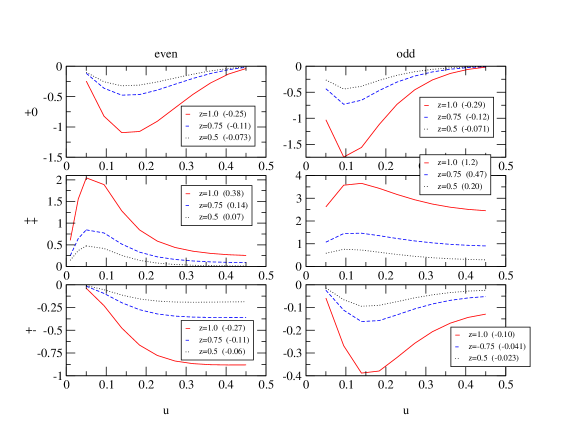
Figure 13: The sensitivity to varying $z$: the six helicity amplitudes differential in $u$. The $y$-axis is $\frac{1}{C_{\rho}}\frac{d{M}_{+i}^{odd/even}}{du}$, where $C_{\rho}=i\hat{s}\alpha_{s}^{IF^{2}}(N^{2}-1/N^{2})eQ_{\rho}f_{\rho}$ and $(m,\,|{\bf q}|)=(m_{\rho}/2,\,\sqrt{10}\,\text{GeV})$.

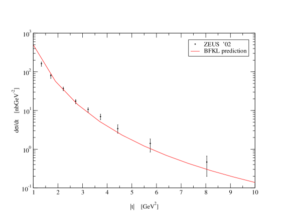
Figure 14: An improved fit: $d\sigma/dt$ for parameter values, $(\alpha_{s}^{IF},\,\alpha_{s}^{BFKL},\,\Lambda^{2},\,m)=(0.17,\,0.25,\,m_{\rho}^{2}-t,\,m_{\rho}/2)$

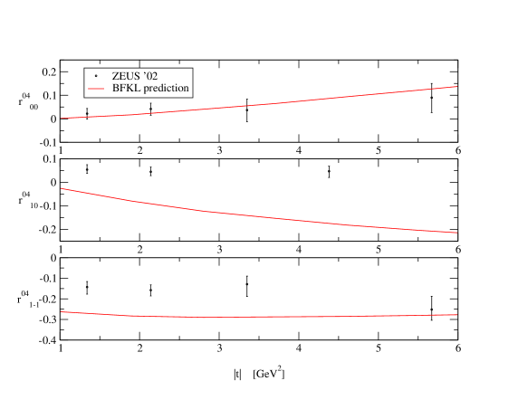
Figure 15: An improved fit: $r$-matrix elements for parameter values, $(\alpha_{s}^{BFKL},\,\Lambda^{2},\,m)=(0.25,\,m_{\rho}^{2}-t,\,m_{\rho}/2)$.

4.4.4 Sensitivity to quark mass

The sensitivity of our BFKL predictions to the quark mass parameter has not so far been explored. We do so now. Figure 16 shows differential cross-section predictions. The central curve is that of the default set, where $(\alpha_{s}^{IF},\,\alpha_{s}^{BFKL},\,\Lambda^{2},\,m)$ $=$ $(0.17,\,0.2,\,m_{\rho}^{2},\,m_{\rho}/2)$. The other two curves were generated by doubling and halving the constituent quark mass. Bearing in mind the fact that we have varied the mass parameter considerably, we see that the cross-section has a fairly robust prediction, its shape being fairly insensitive to changes in $m$.

Figure 17 shows the $r$-matrix element predictions for various quark masses. They are all sensitive to this parameter, both in shape and in normalisation. Figure 18 helps to explain why this is so. It shows the six helicity amplitudes, differential in $u$, for $m=m_{\rho}/4,\,m_{\rho}/2$ and $m_{\rho}$. We point out that it is not in fact the value of $m$ that is significant, it is the value of $m/|{\bf q}|$, and in these plots we fixed $|{\bf q}|=\sqrt{10}$ GeV. Notice that as we increase the scale $m/|{\bf q}|$, the peaks of the distributions become concentrated increasingly toward $u=1/2$, as expected. However, the effect is quite dramatic. Halving the constituent mass strongly enhances the contributions close to the end-points. The effect is particularly marked for the longitudinal helicity amplitudes, since they are forced to zero at exactly $u=1/2$. Raising the quark mass is therefore a mechanism for suppressing the longitudinal components with respect to the transverse. The dramatic dependence of the end-point region on the quark mass, especially for the $M_{++}^{even}$, $M_{+0}^{odd}$ and $M_{+-}^{odd}$ amplitudes, is closely related to the observations of [6] who found that these three amplitudes are divergent in the two-gluon exchange approximation due to divergent end-point behaviour. We here note that although our amplitudes are no longer divergent, even in the massless quark limit, they do retain a memory of these large end-point contributions. We explore the end-point region in much more detail in Appendix B. In passing we note that this physics is reminiscent of that for the DIS process $\gamma e\rightarrow\gamma\gamma^{*}e\rightarrow ef\bar{f}$, where $f$ is a fermion. The structure function $F_{A}^{\gamma}$ is zero at $u=1/2$ and has large contributions close to the end-points that become suppressed as we increase the fermion mass [17].

It is interesting to note that for a large enough $m$, the ${M}_{+0}$ amplitude not only is small but also changes sign. Then, the prediction of $r_{10}^{04}$ flips sign to that of the data. Figure 17 shows this begins to occur for $m$ as low as $m_{\rho}$, in the low $|t|$ region. The evidence of this can also be seen even at large $t$, in Figure 18, where the values of ${M}_{+0}$ differential in $u$, become positive for small $u$. So, increasing $m$ would be a possible mechanism for improving our fits, however, we find it difficult to justify a mass parameter so far away from the constituent mass.

Increasing the mass has the effect of suppressing large dipole configurations due to the McDonald Bessel function, $K_{i}(m|{\bf r}|)$, present in the ${\bf r}$ space representation of the photon wavefunction (e.g. see (15)) which has a large argument suppression $\sim e^{-m|{\bf r}|}$. Figure 18 illustrates the point; larger masses suppress the end-point contributions more strongly. End-point contributions in $u$ correspond to large dipole sizes and the data may therefore be interpreted as suggesting that large dipole sizes should be more heavily suppressed than our calculations predict. The $\delta$-function distribution amplitude that we used in the collinear approximation is an extreme way of achieving this suppression (by forcing $u=1/2$). We suggest that the real physics of this suppression arises as a result of Sudakov factors associated with the quark lines [19].

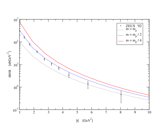
Figure 16: The sensitivity to varying $m$: $d\sigma/dt$ for parameter values, $(\alpha_{s}^{IF},\,\alpha_{s}^{BFKL},\Lambda^{2})$ $=$ $(0.17,\,0.2,\,m_{\rho}^{2})$.

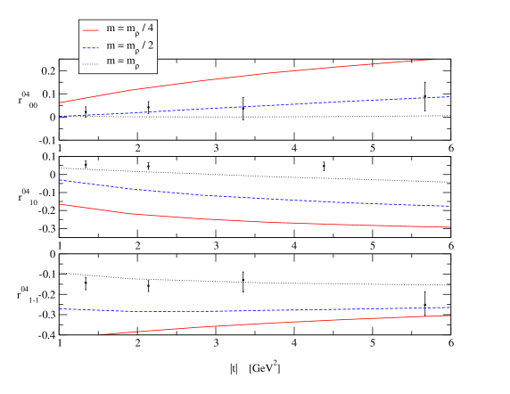
Figure 17: The sensitivity to varying $m$: $r$-matrix elements for parameter values, $(\alpha_{s}^{BFKL},\Lambda^{2})$ $=$ $(0.2,\,m_{\rho}^{2})$.

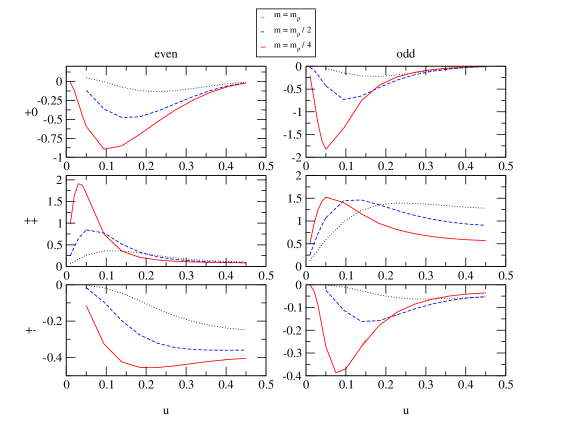
Figure 18: The sensitivity to varying $m$: the six helicity amplitudes differential in $u$. The $y$-axis is $\frac{1}{C_{\rho}}\frac{d{M}_{+i}^{odd/even}}{du}$, where $C_{\rho}=i\hat{s}\alpha_{s}^{IF^{2}}(N^{2}-1/N^{2})eQ_{\rho}f_{\rho}$ and $(z,\,|{\bf q}|)=(0.75,\,\sqrt{10}\,\text{GeV})$.

4.5 Sensitivity to distribution amplitudes

In the next part of our analysis, we examine the effect of subasymptotic corrections to the meson distribution amplitudes. We use the full distribution amplitudes of [12, 13] presented in Appendix A in conjunction with the helicity amplitudes (9)–(14). We remind the reader that we do not adjust any of the parameters of the distribution amplitudes.

Figure 19 shows the differential cross-section in two distribution amplitude prescriptions which we label “asymptotic” and “BBKT” (Ball, Braun, Koike, Tanaka). The more accurate distribution amplitudes prove to make no qualitative difference. Figure 20, for the $r$ matrix elements, show that the effects are quite modest in these ratios.

Figure 21 shows the six helicity amplitudes, differential in $u$, at fixed rapidity $z=0.75$. Referring back to the amplitudes ${M}_{++}^{even}$ and ${M}_{+-}^{even}$, given by (10) and (11), we see that the difference between their $u$ dependence is a relative switch in sign between two pieces (one corresponding to the vector component of the Fierz decomposition and the other to the pseudovector). The plots in Figure 21 demonstrate a cancellation in the effects of the non-asymptotic distribution amplitudes for ${M}_{++}^{even}$, but an amplification for ${M}_{+-}^{even}$. The effects of the different distribution amplitudes on the $u$ distributions of the amplitudes are most significant for ${M}_{+-}^{even}$ and ${M}_{++}^{odd}$. However, even then there is a significant cancellation in their integrated values. We note that subasymptotic corrections are no aid to improving our fit to $r_{10}^{04}$.

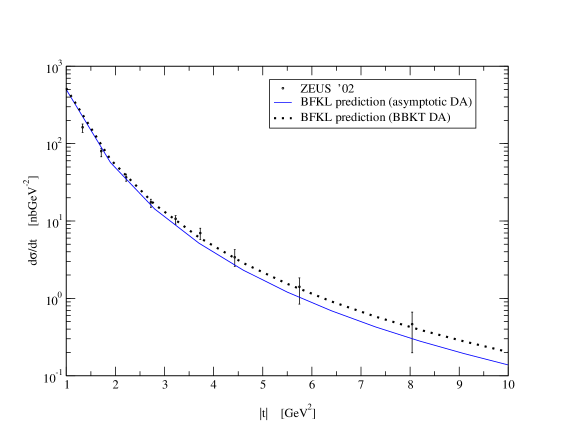
Figure 19: The effect sub-asymptotic distribution amplitudes [12, 13]: $d\sigma/dt$ for parameter values, $(\alpha_{s}^{IF},\,\alpha_{s}^{BFKL},\,\Lambda^{2},\,m)$ $=$ $(0.17,\,0.25,\,m_{\rho}^{2}-t,\,m_{\rho}/2)$

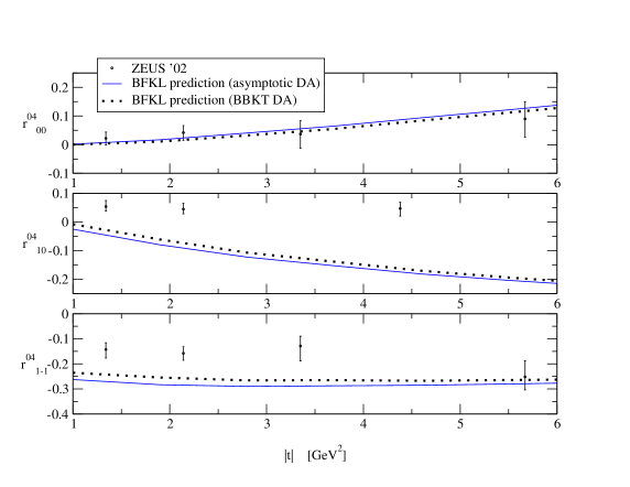
Figure 20: The effect of sub-asymptotic distribution amplitudes [12, 13]: $r$-matrix elements for parameter values, $(\alpha_{s}^{BFKL},\,\Lambda^{2},\,m)$ $=$ $(0.25,\,m_{\rho}^{2}-t,\,m_{\rho}/2)$

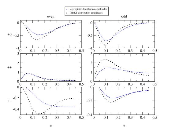
Figure 21: The effect of sub-asymptotic distribution amplitudes [12, 13]: the six helicity amplitudes differential in $u$. The $y$-axis is $\frac{1}{C_{\rho}}\frac{d{M}_{+i}^{odd/even}}{du}$, where $C_{\rho}=i\hat{s}\alpha_{s}^{IF^{2}}(N^{2}-1/N^{2})eQ_{\rho}f_{\rho}$ and $(z,\,m,\,|{\bf q}|)=(0.75,\,m_{\rho}/2,\,\sqrt{10}\,\text{GeV})$.

Before proceeding, we ought to comment that in our approach it is assumed that the dipoles which scatter elastically at high $t$ are small in comparison to the meson size. Therefore the dependence of the vector meson wavefunction on the dipole size is neglected. On the other hand, we use the perturbative photon wavefunction, with a constituent quark mass giving the upper cut-off of the dipole sizes in the photon (recall, that $K_{a}(mr)\to\exp(-mr)$ for $mr\gg 1$). Sensitivity of the amplitudes to this parameter turns out to be significant. This suggests that an additional suppression of larger dipoles by the transverse part of the vector meson wave function could well have a sizeable effect.

5 Phenomenology for the $\rho$, $\phi$ and $J/\psi$

We now turn our attention to the $\phi$ and $J/\psi$, reverting to the use of the asymptotic distribution amplitudes since wish to treat the three mesons on the same footing. Given the smallness of the sub-asymptotic corrections for the $\rho$ (as illustrated in the previous section) this seems quite reasonable.

To what extent do the observations, made for the $\rho$ in the preceding sections, hold for the other mesons? The calculation for a general meson, $V$, with asymptotic distribution amplitude, requires only the substitution $(f_{\rho}/f_{\rho}^{T},\,Q_{\rho},\,m_{\rho})$ $\rightarrow$ $(f_{V}/f_{V}^{T},\,Q_{V},\,m_{V})$. The values for the meson decay constant ($f_{V}$) and electromagnetic coupling ($Q_{V}$) are constants of proportionality. $m_{V}$ appears in the BFKL logarithm and the $\gamma V$ impact factor (through the quark mass $m=m_{V}/2$), and is qualitatively the most significant parameter. The mass of the $\phi$ is similar to that of the $\rho$, while the mass of the $J/\psi$ is significantly larger. We might therefore expect the predictions for the $\phi$ to be, qualitatively, similar to the $\rho$, and those for the $J/\psi$ to be, perhaps, very different. This is in fact what we shall see.

Figures 22 and 23 reproduce our ‘improved fit’ prediction for the $\rho$ shown in Figure 14, where we played off the effects or adjusting $\alpha_{s}^{BFKL}$ and $\Lambda^{2}$ to our advantage. Now we also show the two-gluon exchange predictions. Two-gluon exchange with a fixed strong coupling predicts a differential cross-section far too flat in $|t|$. Running the coupling solves this problem and provides a good fit. However, looking at the two-gluon predictions for the $r$-matrix elements (which are independent of how we treat $\alpha_{s}^{IF}$), we see that the values for the $r_{00}^{04}$ far exceed those constrained by the data. This means that the longitudinal component dominates for two-gluon exchange. This is in line with our observation that the longitudinal fraction increases as we lower the $z$ rapidity (recall that the BFKL solution tends to two-gluon exchange in the limit $z\rightarrow 0$) and is illustrated explicitly in Figure 24. Thus, even though we have succeeded in getting the two-gluon curve to agree with the data for $d\sigma/dt$ it is generated by fundamentally wrong dynamics. We do however note the improvement with respect to working within the collinear and $\delta$-function distribution amplitude approximation. In that prescription, two-gluon exchange was studied in [8, 3]. The dip to zero manifest at $|t|=m_{V}^{2}$ is not seen in data and is a somehwat artificial prediction arising from the crudity of the treatment of the meson distribution amplitudes.

Figures 25–26 and 27–28 present our results for the $\phi$ and $J/\psi$ mesons. The BFKL curves which we label “(1)” in Figures 25 and 27 were obtained by simply making the appropriate change in meson constants and masses. No further adjustment of the other parameters is made relative to the fit for the $\rho$ meson. For the curves labelled “BFKL (2)” we altered the values of the meson tensor coupling but have kept the ratio

$$f_{V}^{T}=\frac{f_{\rho}^{T}}{f_{\rho}}f_{V}.$$ (26)

Fixing $f_{V}^{T}$ in this way improves the fit to data. Note that if we allowed ourselves slightly more freedom with the values of $f_{V}^{T}$, the quality of the fits to the $t$-distribution could be improved still further.

The $\phi$ predictions are similar to those for the $\rho$. We again see that the two-gluon exchange $t$-distribution requires a running strong coupling to fit the data and that the $r$-matrix elements point to this being an accident. The BFKL predictions are again correctly dominated by the transverse contributions, but again fail to predict the correct sign for $r^{04}_{10}$ in the case of the $\phi$. However, for the $J/\psi$, the BFKL predictions are compatible with all the observables. The large quark mass drives the longitudinal amplitudes small enough to agree with the $r^{04}_{10}$ data. We note that although the two-gluon exchange $r$-matrix predictions for the $J/\psi$ are in marginal agreement with the data, we have to doubt the validity of the underlying dynamics, given the comments above.

Comparing two-gluon exchange and BFKL predictions, we see that the BFKL calculation is a definite step forward. The success of the our predictions for the $\phi$ and $J/\psi$ is a noteworthy result. We now understand the success of the apparently naive analysis of [8] as being due to the fact that it correctly identified the dominance of the ${M}^{odd}_{++}$ amplitude. However, the inability of BFKL to agree with the data for $r_{10}^{04}$ suggests that while the longitudinal contribution is brought down by BFKL effects, it is still not under enough control to accurately describe all the observables measured at ZEUS and H1.

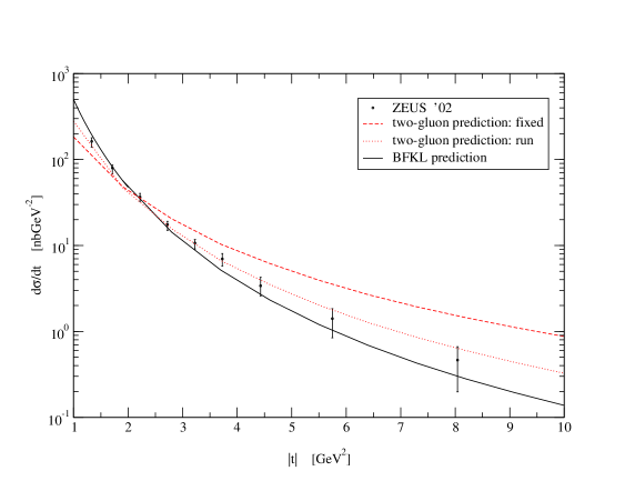
Figure 22: $\rho$ photoproduction: $d\sigma/dt$. The fixed two-gluon curve was calculated with the parameter values $(\alpha_{s}^{IF},\,f_{\rho},\,f_{\rho}^{T},\,m)$ $=$ $(0.27,\,0.216\,\text{GeV},\,$ $0.160\,\text{GeV},\,m_{\rho}/2)$. The run two-gluon curve was calculated with the parameter values $(\alpha_{s}^{IF}(1\,\text{GeV}),\,f_{\rho},\,f_{\rho}^{T},\,m)$ =$(0.30,\,0.216\,\text{GeV},\,0.160\,\text{GeV},\,m_{\rho}/2)$. The BFKL calculated for the parameter values $(\alpha_{s}^{IF},\,\alpha_{s}^{BFKL},\,\Lambda^{2},\,f_{\rho},\,f_{\rho}^{T},\,m)$ $=$ $(0.17,\,0.25,\,m_{\rho}^{2}-t,\,0.216\,\text{GeV},\,$ $0.160\,\text{GeV},\,m_{\rho}/2)$.

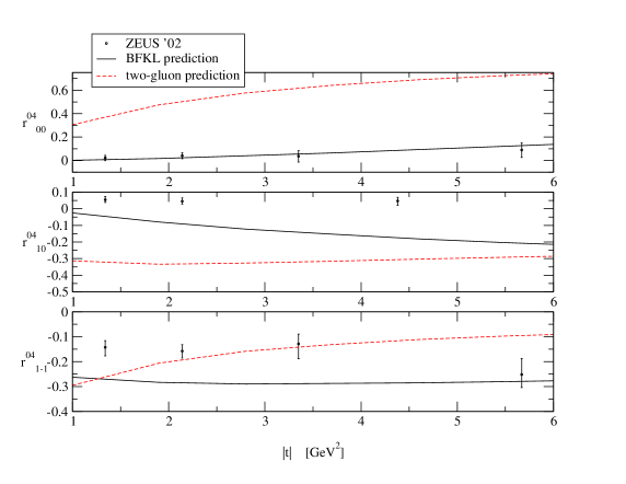
Figure 23: $\rho$ photoproduction: $r$-matrix elements. The two-gluon curve was calculated with the parameter values $(f_{\rho},\,f_{\rho}^{T},\,m)$ = $(0.216\,\text{GeV},\,0.160\,\text{GeV},\,m_{\rho}/2)$. The BFKL curve was calculated for the parameter values $(\alpha_{s}^{BFKL},\,\Lambda^{2},\,f_{\rho},\,f_{\rho}^{T},\,m)$ $=$ $(0.25,\,m_{\rho}^{2}-t,\,0.216\,\text{GeV},\,$ $0.160\,\text{GeV},\,m_{\rho}/2)$.

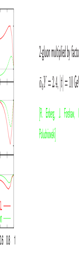
Figure 24: The relative contributions for two-gluon exchange and full BFKL ($z=1.2$,
$t=-10$ GeV²): the six helicity amplitudes differential in $u$. Note that the two-gluon exchange results have been multiplied by a factor of 3.

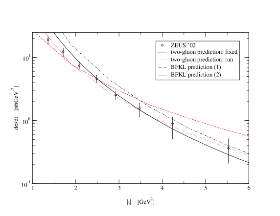
Figure 25: $\phi$ photoproduction: $d\sigma/dt$ for parameter values. The fixed two-gluon curve was calculated with the parameter values $(\alpha_{s}^{IF},\,f_{\phi},\,f_{\phi}^{T},\,m)$ $=$ $(0.25,\,0.231\,\text{GeV},\,$ $0.215\,\text{GeV},\,m_{\phi}/2)$. The run two-gluon curve was calculated with the parameter values $(\alpha_{s}^{IF}(1\,\text{GeV}),\,$ $f_{\phi},\,f_{\phi}^{T},\,m)$ $=$ $(0.28,\,0.231\,\text{GeV},\,$ $0.215\,\text{GeV},\,m_{\phi}/2)$. BFKL prediction $(1)$ is for the parameter values $(\alpha_{s}^{IF},\,\alpha_{s}^{BFKL},\,$ $\Lambda^{2},\,f_{\phi},\,f_{\phi}^{T},\,m)$ $=$ $(0.17,\,0.25,\,m_{\phi}^{2}-t,\,$ $0.231\,\text{GeV},\,$ $0.215\,\text{GeV},\,m_{\phi}/2)$. BFKL prediction $(2)$ is for the parameter values $(\alpha_{s}^{IF},\,\alpha_{s}^{BFKL},\,\Lambda^{2},\,f_{\phi},\,f_{\phi}^{T},\,m)$ $=$ $(0.17,\,0.25,\,m_{\phi}^{2}-t,\,$ $0.231\,\text{GeV},\,$ $0.171\,\text{GeV},\,m_{\phi}/2)$.

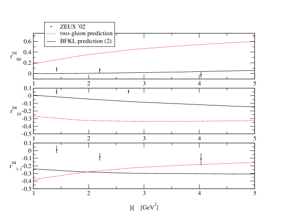
Figure 26: $\phi$ photoproduction: $r$-matrix element. The fixed two-gluon curve was calculated with the parameter values $(f_{\phi},\,f_{\phi}^{T},\,m)$ $=$ $(0.231\,\text{GeV},\,$ $0.215\,\text{GeV},\,m_{\phi}/2)$. The BFKL prediction ($(2)$) is for the parameter values $(\alpha_{s}^{BFKL},\,\Lambda^{2},\,$ $f_{\phi},\,f_{\phi}^{T},\,m)$ $=$ $(0.25,\,m_{\phi}^{2}-t,\,$ $0.231\,\text{GeV},\,$ $0.171\,\text{GeV},\,m_{\phi}/2)$.

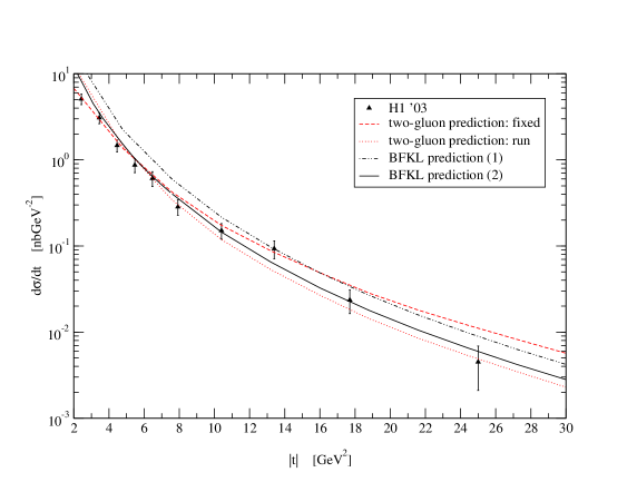
Figure 27: $J/\psi$ photoproduction: $d\sigma/dt$. The fixed two-gluon curve was calculated with the parameter values $(\alpha_{s}^{IF},\,f_{J/\psi},\,f_{J/\psi}^{T},\,m)$ $=$ $(0.23,\,0.405\,\text{GeV},\,$ $0.405\,\text{GeV},\,m_{J/\psi}/2)$. The run two-gluon curve was calculated with the parameter values $(\alpha_{s}^{IF}(1\,\text{GeV})\,$ $f_{J/\psi},\,f_{J/\psi}^{T},\,m)$ $=$ $(0.29,\,0.405\,\text{GeV},\,$ $0.405\,\text{GeV},\,m_{J/\psi}/2)$. BFKL prediction $(1)$ is for the parameter values $(\alpha_{s}^{IF},\,\alpha_{s}^{BFKL},\,$ $\Lambda^{2},\,$ $f_{J/\psi},\,f_{J/\psi}^{T},\,m)$ $=$ $(0.17,\,0.25,\,m_{J/\psi}^{2}-t,\,0.405\,\text{GeV},\,$ $0.405\,\text{GeV},\,m_{J/\psi}/2)$. BFKL prediction $(2)$ is for the parameter values $(\alpha_{s}^{IF},\,\alpha_{s}^{BFKL},\,\Lambda^{2},\,$ $f_{J/\psi},\,f_{J/\psi}^{T},\,m)$ $=$ $(0.17,\,0.25,\,m_{J/\psi}^{2}-t,\,0.405\,\text{GeV},\,$ $0.300\,\text{GeV},\,m_{J/\psi}/2)$.

Figure 28: $J/\psi$ photoproduction: $r$-matrix elements. The two-gluon curve was calculated with the parameter values $(f_{J/\psi},\,f_{J/\psi}^{T},\,m)$ $=$ $(0.405\,\text{GeV},\,$ $0.405\,\text{GeV},\,m_{J/\psi}/2)$. The BFKL prediction ($(2)$) is for the parameter values $(\alpha_{s}^{BFKL},\,\Lambda^{2},\,$ $f_{J/\psi},\,f_{J/\psi}^{T},\,m)$ $=$ $(0.25,\,m_{J/\psi}^{2}-t,\,0.405\,\text{GeV},\,$ $0.300\,\text{GeV},\,m_{J/\psi}/2)$.

6 Summary

We have compared our theoretical predictions for $d\sigma/dt$ and the three $r$-matrix elements to the data of ZEUS and H1, in various levels of approximation. The only meson we found complete agreement for, in any scheme, was the $J/\psi$. We nevertheless could generally obtain good fits to the $r_{00}^{04}$ observable. Fits to the cross-sections favoured running the BFKL scale in a natural way: $\Lambda^{2}=m_{V}^{2}-t$. The theoretical predictions for $r^{04}_{10}$ were the main obstacles to obtaining satisfactory fits for the $\rho$ and $\phi$. We found the natural predictions of both two-gluon and BFKL pomeron exchange to be the wrong sign. The predictions of the observables proved insensitive to higher twist terms, suggesting that these corrections are unlikely to provide a solution. We also found that using the distribution amplitudes of [12, 13] had little effect on the quality of fits compared to the asymptotic ones. The inability of theoretical predictions to fit $r_{10}^{04}$, and the general sensitivity of the $r$-matrix elements to the quark mass parameter, $m$, therefore seem to locate the problem at the level of the hard subprocess. We suggest that the data hint that we may require a greater suppression of larger dipoles than we predict and that this may be provided by Sudakov suppression of emissions off the quark lines.

We note the dominance of the ${M}_{++}^{odd}$ contribution and have demonstrated that this corresponds to the amplitude used in the BFKL calculation of [8] (which was, in addition, conducted in a $\delta$-function approximation). We were able to get excellent agreement for the $\phi$ and $J/\psi$ differential cross-sections $using$ $the$ $same$ $parameters$ that fitted the $\rho$. On the whole the evidence suggests that leading logarithm BFKL predictions work well for the transverse amplitudes but, despite suppressing the longitudinal component relative to Born level, it fails to have enough control over this contribution.

Dedication and Acknowledgements

We should like to dedicate this paper to the memory of Jan Kwiecinski, a good friend, colleague and inspirational teacher.

RE wishes to thank the Theoretical Physics Group at the University of Manchester for their hospitality when parts of this work was carried out. LM is grateful to Gunnar Ingelman and the Uppsala THEP group for their warm hospitality. This research was funded in part by the UK Particle Physics and Astronomy Research Council (PPARC), by the Swedish Research Council, and by the Polish Committee for Scientific Research (KBN) grant no. 5P03B 14420.

Appendix A Vector meson distribution amplitudes

The authors of [12] presented results for the complete set of distribution amplitudes up to twist-3 for the $\rho$ and $\phi$ (and $K$) [12]. These results were extended to twist-4 in [13]. The relevant distribution amplitudes, up to and including twist-4, are classified in Table 4.

	Twist 2	Twist 3	Twist 4
	$O(1)$	$O(1/q)$	$O(1/q^{2})$
$\|$	$\phi_{\|}$	$h_{\|}^{(t)},\,h_{\|}^{(s)}$
$\perp$	$\phi_{\perp}$	$g_{\perp}^{(v)},\,g_{\perp}^{(a)}$	$h_{3}$

Table 4: Classification of distribution amplitudes up to twist-4.

We quote all parameters at the renormalisation scale $\mu^{2}=1\,\text{GeV}^{2}$ and neglect the slow running. In the $q\rightarrow\infty$ limit, the parameters vanish. We refer to this as the asymptotic limit, and the distribution amplitudes in this limit as the asymptotic distribution amplitudes.

Tables 5 and 6 hold the values of all the relevant parameters, at the scale $\mu^{2}=1\,\text{GeV}^{2}$.

	$a_{1}^{\|}$	$a_{2}^{\|}$	$\zeta_{3}$	$\omega_{3}^{A}$	$\omega_{3}^{V}$
$\rho$	$0$	$0.18\pm 0.10$	$0.032\pm 0.010$	$-2.1\pm 1.0$	$3.8\pm 1.8$

Table 5: Chiral even parameters: $\mu^{2}=1\,\text{GeV}^{2}$.

	$a_{1}^{\perp}$	$a_{2}^{\perp}$	$\zeta_{3}$	$\omega_{3}^{T}$	$\zeta_{4}^{T}$	$\tilde{\zeta}_{4}^{T}$
$\rho$	$0$	$0.20\pm 0.10$	$0.032\pm 0.010$	$7.0\pm 7.0$	$0.10\pm 0.05$	$-0.10\pm 0.05$

Table 6: Chiral odd parameters: $\mu^{2}=1\,\text{GeV}^{2}$.

We do not include quark mass corrections in this study. They are in any case zero for the $\rho$ meson.

A.1 Twist-2 distribution amplitudes

A.1.1 Chiral Even

There is one chiral even, twist-2 amplitude:

$$\phi_{\|}(u)=6u\bar{u}\left(1+3a_{1}^{\|}\xi+a_{2}^{\|}\,\frac{3}{2}(5\xi^{2}-1)\right).$$ (27)

and the asymptotic distribution is

$$\phi_{\|}^{asy}(u)=6u\bar{u}.$$ (28)

A.1.2 Chiral Odd

There is one chiral odd, twist-2 amplitude. This can be written

$$\phi_{\perp}(u)=6u\bar{u}\left(1+3a_{1}^{\perp}\xi+a_{2}^{\perp}\,\frac{3}{2}(5\xi^{2}-1)\right).$$ (29)

The asymptotic distribution is

$$\phi_{\|}^{asy}(u)=6u\bar{u}.$$ (30)

A.2 Twist-3 distribution amplitudes

A.2.1 Chiral Even

There are two even, twist-3 distributions:

$$g_{\perp}^{(a)}(u)=6u\bar{u}\left[1+\left\{\frac{1}{4}a_{2}^{\|}+\frac{5}{3}\zeta_{3}\left(1-\frac{3}{16}\omega_{3}^{A}+\frac{9}{16}\omega_{3}^{V}\right)\right\}(5\xi^{2}-1)\right]$$ (31)

and

$$g_{\perp}^{(v)}(u)=\frac{3}{4}(1+\xi^{2})+(\frac{3}{7}a_{2}^{\|}+5\zeta_{3})\,(3\xi^{2}-1)$$

$$+\left[\frac{9}{112}a_{2}^{\|}+\frac{15}{64}\zeta_{3}(3\omega_{3}^{V}-\omega_{3}^{A})\right](3-30\xi^{2}+35\xi^{4})$$ (32)

where the subscript of ‘$3$’ refers to three-particle corrections and we neglect mass corrections. In the asymptotic limit

$$g_{\perp}^{(a)\,asy}(u)=6u\bar{u}.$$ (33)

and

$$g_{\perp}^{(v)\,asy}(u)=\frac{3}{4}\,(1+\xi^{2}).$$ (34)

A.2.2 Chiral Odd

There is one relevant chiral odd twist-3 distribution:

$$h_{\|}^{(t)}(u)=3\xi^{2}+\frac{3}{2}\,a_{2}^{\perp}\,\xi^{2}(5\xi^{2}-3)+\frac{15}{16}\,\zeta_{3}\,\omega_{3}^{T}(3-30\xi^{2}+35\xi^{4}).$$ (35)

In the asymptotic limit

$$h_{\|}^{(t)\,asy}(u)=3\xi^{2}.$$ (36)

A.3 Twist-4 distribution amplitudes

A.3.1 Chiral Odd

There is one relevant chiral odd twist-4 distribution;

$$h_{3}(u)=1+\left(-1+\frac{3}{7}a_{2}^{\perp}-10(\zeta_{4}^{T}+\tilde{\zeta}_{4}^{T})\right)C_{2}^{1/2}(\xi)$$

$$\hskip 113.81102pt+\left(-\frac{3}{7}a_{2}^{\perp}-\frac{15}{8}\zeta_{3}\omega_{3}^{T}\right)C_{4}^{1/2}(\xi).$$ (37)

where $C_{n}^{\lambda}(\xi)$ are Gegenbauer polynomials. In the asymptotic limit

$$h_{3}^{asy}=1-C_{2}^{1/2}(\xi)=\frac{3}{2}(1-\xi^{2}).$$ (38)

A.4 Distribution amplitude schemes

We have six helicity amplitudes to consider, i.e. (9)–(14). Their individual dependence on the distribution amplitudes is as follows:

$$\Phi_{+0}^{even}(u)\equiv\phi_{\|}(u)$$ (39)

$$\Phi_{++}^{even}(u)\equiv\left(\frac{g_{\perp}^{(a)}(u)}{4}-(1-2u)\int_{0}^{u}dv\,(\phi_{\|}(v)-g_{\perp}^{(v)}(v))\right)$$ (40)

$$\Phi_{+-}^{even}(u)\equiv\left(\frac{g_{\perp}^{(a)}(u)}{4}+(1-2u)\int_{0}^{u}dv\,(\phi_{\|}(v)-g_{\perp}^{(v)}(v))\right)$$ (41)

$$\Phi_{+0}^{odd}(u)\equiv\int_{0}^{u}dv\,\left(h_{\|}^{(t)}(v)-\phi_{\perp}(v)\right)$$ (42)

$$\Phi_{++}^{odd}(u)\equiv\phi_{\perp}(u)$$ (43)

$$\Phi_{+-}^{odd}(u)\equiv\int_{0}^{u}dv\int_{0}^{v}d\eta\left(h_{\|}^{(t)}(\eta)-\frac{1}{2}\phi_{\perp}(\eta)-\frac{1}{2}h_{3}(\eta)\right).$$ (44)

We now present the explicit formulae for these amplitudes in four different prescriptions.

A.4.1 Prescription 1: leading twist (collinear) approximation with $\delta$-function distributions

We keep only the twist-2 contributions and equate the corresponding distribution amplitudes to a $\delta$-function that enforces the quark and antiquark share the meson momentum equally. Then

$$\Phi_{+0}^{even}(u)=\delta\left(u-\frac{1}{2}\right)$$ (45)

$$\Phi_{++}^{even}(u)=0$$ (46)

$$\Phi_{+-}^{even}(u)=0$$ (47)

$$\Phi_{+0}^{odd}(u)=0$$ (48)

$$\Phi_{++}^{odd}(u)=\delta\left(u-\frac{1}{2}\right)$$ (49)

$$\Phi_{+-}^{odd}(u)=0.$$ (50)

A.4.2 Prescription 2: leading twist (collinear) approximation with asymptotic distribution amplitudes

We keep only the twist-2 contributions and equate the corresponding distribution amplitudes to their asymptotic forms. Then

$$\Phi_{+0}^{even}(u)=6u\bar{u}$$ (51)

$$\Phi_{++}^{even}(u)=0$$ (52)

$$\Phi_{+-}^{even}(u)=0$$ (53)

$$\Phi_{+0}^{odd}(u)=0$$ (54)

$$\Phi_{++}^{odd}(u)=6u\bar{u}$$ (55)

$$\Phi_{+-}^{odd}(u)=0.$$ (56)

A.4.3 Prescription 3: higher twist approximation with asymptotic distribution amplitudes

We keep all twist and equate the corresponding distribution amplitudes to the asymptotic forms. After integration:

$$\Phi_{+0}^{even}(u)=6u\bar{u}$$ (57)

$$\Phi_{++}^{even}(u)=3u\bar{u}(u^{2}+\bar{u}^{2})$$ (58)

$$\Phi_{+-}^{even}(u)=6u^{2}\bar{u}^{2}$$ (59)

$$\Phi_{+0}^{odd}(u)=3(1-2u)u\bar{u}$$ (60)

$$\Phi_{+-}^{odd}(u)=\frac{3}{2}u^{2}\bar{u}^{2}$$ (61)

A.4.4 Prescription 4: higher twist approximation with BBKT distribution amplitudes

We keep all twist and equate the corresponding distribution amplitudes to the BBKT forms listed in A1–A3. We neglect to explicitly quote the trivial, but bulky, integrated forms.

Appendix B End-point behaviour

B.1 Two-gluon exchange and Reggeisation corrections

The importance of contributions at, and close to, end-points is a matter of debate (see for example ([6, 7, 23])). The authors of [6] worked in the two-gluon exchange approximation in the light-quark limit and concluded that $M_{++}^{even}$, $M_{+0}^{odd}$ and $M_{+-}^{odd}$ were all plagued by end-point divergences. They argued that these end-point divergences would be brought under control by Sudakov corrections and hence that the dominant amplitude would remain $M_{++}^{odd}$. In [7], the end-point divergences were interpreted as the signal that QCD factorisation was breaking down. In the context of a specific model of the vector meson wavefunction, [23] obtain a meson wavefunction, dependent on both longitudinal and transverse coordinates, by a Borel transform of the photon wavefunction. The model of [23] gives an explicit form for the end-point contributions at all twist, it is shown that those contributions can be resummed and that the breakdown of factorisation by end-point divergencies at leading twist is only apparent. Here we discuss the role of end-points within the context of leading logarithmic BFKL resummation.

In Figure 16, we also observe the appearance of large end-point contributions (in the same amplitudes noted by [6]). It is the case that these contributions lead to divergent matrix elements in the two-gluon approximation in the case of massless quarks. However, these divergences are not present after re-summing the BFKL logarithms. In Figure 29 we show that the the BFKL prediction for the $(++)$ amplitude remains finite even in the massless quark limit. We shall investigate how this divergence in (++) at the Born level arises and how higher orders bring it under control. The authors of [6] worked with the asymptotic distribution amplitudes; we shall also do so (see Appendix A for the asymptotic formulae). The end-point behaviour is independent of this approximation.

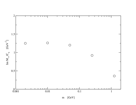
Figure 29: The ${M}_{++}^{even}$ amplitude against $m$, the quark mass parameter. The fixed parameter values are $(z,m_{V},|t|)=(1.0,m_{\rho},10\,\text{GeV}^{2})$. The constant, $C_{q}=s\alpha_{s}^{2}(N^{2}-1/N^{2})f_{V}m_{V}ee_{q}$ and the asymptotic distribution amplitudes were used.

The light-quark limit corresponds to putting the mass of the quarks that form the meson to zero. This leads to the replacements

$$mK_{1}(m|r|)\rightarrow 1/|r|\hskip 14.22636pt\text{and}\hskip 14.22636ptK_{0}(m|r|)\rightarrow-m\text{ln}(m|r|)\sim 0,$$ (62)

where we have assumed that $m|r|\rightarrow 0$, i.e. that we get no significant contributions from asymptotically large transverse sizes.

We can apply the light quark approximation to the Born (two-gluon) level amplitudes previously derived. For $M^{even\,2g}_{++}$ one has

$${M}^{even\,2g}_{++}=-sC_{V}f_{V}M_{V}\frac{6\pi}{|{\bf q}|^{4}}\left(\text{ln}\left(\frac{1-u_{min}}{u_{min}}\right)-1+2u_{min}\right).$$ (63)

A clear divergence as the cut-off $u_{min}\to 0$.

The full BFKL solution has proven in the past to improve infra-red finiteness of scattering amplitudes; see for example [20, 21] for the case of $qq\rightarrow qq$ scattering. At any finite order in $\alpha_{s}$ this scattering amplitude diverges. Even in infra-red finite observables the Born level result can be seen to give undue weight to contributions from momentum configurations which are unphysical, i.e. where all the momentum is short-circuited down one gluon.

The authors of [3] demonstrated how this problem can be resolved without recourse to the full BFKL result, but rather by a fixed order resummation of a subset of the BFKL logarithms. Following [3], we go from the Born amplitude to the resummed one by the substitution

$$\frac{1}{{\bf{\bf k}}^{2}({\bf{\bf k}}-{\bf{\bf q}})^{2}}\rightarrow\frac{1}{{\bf{\bf k}}^{2}({\bf{\bf k}}-{\bf{\bf q}})^{2}}\left(\frac{{\bf{\bf k}}^{2}({\bf{\bf k}}-{\bf{\bf q}})^{2}}{{\bf q}^{4}}\right)^{z}.$$ (64)

The substitution above clearly suppresses small gluon momenta and the formerly divergent amplitude can now be written (using the definition of the incomplete beta function)

$${M}^{even\,2gR}_{++}=-\frac{6\pi}{|{\bf q}|^{4}}sC_{V}f_{V}M_{V}$$

$$\times\biggl{[}B(1-u_{min},2z,1+2z)-B(1-u_{min},1+2z,1+2z)\biggr{]}_{u_{min}}^{1-u_{min}}.$$ (65)

We can safely put $u_{min}\rightarrow 0$ for $z>0$:

$${M}^{even\,2gR}_{++}=-\frac{6\pi}{|{\bf q}|^{4}}sC_{V}f_{V}M_{V}\,\left(B(2z,1+2z)-B(1+2z,1+2z)\right)$$

$$=-\frac{6\pi}{|{\bf q}|^{4}}sC_{V}f_{V}M_{V}\,\frac{\Gamma(2z)\Gamma(2+2z)}{\Gamma(2+4z)}.$$ (66)

As it should be, we recover the divergence in the limit $z\rightarrow 0$:

$${M}^{even\,2gR}_{++}(z\rightarrow 0)\rightarrow-\frac{3\pi}{|{\bf q}|^{4}}sC_{V}f_{V}M_{V}\frac{1}{z}.$$ (67)

We observe that this is equal to that derived for $qq\rightarrow qq$ scattering amplitude in [20, 21], excepting a factor of $-3C_{V}f_{V}M_{V}/2q^{2}$. This is understood since in this limit the quark and antiquark are far apart and the dominant contribution comes from coupling the exchanged reggeised gluons to a single parton [3, 22]. The clear result is that the resummed $(++)$ even amplitude remains finite even in the massless quark limit for non-zero rapidity. We have demonstrated analytically that higher orders accomplish this and so it is no longer surprising that Figure 29 demonstrates convergence at $m\to 0$.

B.2 BFKL

The previous subsection is sufficient to illustrate that the BFKL result is free from infrared divergences. Here we take a closer look at the end-point behaviour of the full BFKL amplitude. The reader not interested in the details may wish to jump directly to the final result, (84). Equation (9) and the definition of the asymptotic distributions in Appendix A give us the result

$${M}_{++}^{even}=\frac{sC_{V}f_{V}M_{V}}{8|q|}\,\int_{0}^{1}du\;3\,u\bar{u}\,(u^{2}+\bar{u}^{2})$$

$$\times\sum_{n=-\infty}^{n=+\infty}\int_{-\infty}^{\infty}d\nu\frac{\nu^{2}+n^{2}}{[\nu^{2}+(n-1/2)^{2}][\nu^{2}+(n+1/2)^{2}]}\frac{\exp[\chi_{2n}(\nu)z]}{\sin(i\pi\nu)}\,I_{00}(\nu,2n,q,u;1)$$

(68)

where

$$I_{\alpha\beta}(\nu,n,q,u;a)=\frac{m}{2}\int^{C^{\prime}+i\infty}_{C^{\prime}-i\infty}\frac{d\zeta}{2\pi i}\Gamma(a/2-\zeta)\Gamma(-a/2-\zeta)\,\tau_{q}^{\zeta}\;(i\,\text{sign}\,(1-2u))^{\alpha-\beta+n}$$

$$\times\left(\frac{4}{|q|}\right)^{4}\left[\sin\pi(\alpha+\mu+\zeta)\;\right.B(\alpha,\mu,q^{*},u,\zeta)\,B(\beta,\widetilde{\mu},q,u^{*},\zeta)$$

$$\hskip 56.9055pt-(-1)^{n}\sin\pi(\alpha-\mu+\zeta)\;B(\alpha,-\mu,q^{*},u,\zeta)\,B(\beta,-\widetilde{\mu},q,u^{*},\zeta)\left.\right]$$ (69)

and

$$B(\alpha,\mu,q^{*},u,\zeta)=(-4u\bar{u})^{-(\mu+2+\alpha+\zeta)/2}\left(\frac{4}{q^{*}}\right)^{\alpha}2^{-\mu}\,\frac{\Gamma(\mu+2+\alpha+\zeta)}{\Gamma(\mu+1)}$$

$${}_{2}F_{1}\left(\frac{\mu+2+\alpha+\zeta}{2}\,,\,\frac{\mu-1-\alpha-\zeta}{2}\,;\,\mu+1\,;\,\frac{1}{4u\bar{u}}\right),$$ (70)

with $\tau_{q}=4m^{2}/|q|^{2}$.

The even amplitudes have $a=1$ so the integrand in $I_{\alpha\beta}(\nu,n,q,u;1)$ has a pole at $\zeta=-1/2$, where $-1<C^{\prime}<-1/1$. If we shift the contour to the right we pick up pole contributions from $\text{Re}\,\zeta\geq-1/2$. In the limit $m\rightarrow 0$ we might expect the leading pole to be that at $\zeta=-1/2$, the residue of which is independent of $m$, the other poles contributions vanishing in the limit. The integrand is complicated, however, expressed how it is in terms of blocks of hypergeometric functions. It is difficult to see clearly the analytic behaviour in $\zeta$. For example the true expansion parameter may not be $4m^{2}/q^{2}$, rather something like $4m^{2}/u^{2}q^{2}$, where it is not clear whether the ‘leading pole’ actually is leading in the simultaneous limit $m\rightarrow 0$ and $u\rightarrow 0$. We shall see if some manipulation of the formula can be enlightening. Using the following hypergeometric identity

$${}_{2}F_{1}(a,b;c;z)= \frac{\Gamma(c)\Gamma(b-a)}{\Gamma(b)\Gamma(c-a)}(-z)^{-a}\,{}_{2}F_{1}(a,a+1-c;a+1-b;1/z)$$ (71)

$$+\frac{\Gamma(c)\Gamma(a-b)}{\Gamma(a)\Gamma(c-b)}(-z)^{-b}\,{}_{2}F_{1}(b,b+1-c;b+1-a;1/z),$$

we can re-write,

$$B(\alpha,\mu,q^{*},u,\zeta)=(-4u\bar{u})^{-(\mu+2+\alpha+\zeta)/2}\left(\frac{4}{q^{*}}\right)^{\alpha}2^{-\mu}\,\Gamma(\mu+2+\alpha+\zeta)$$

$$\times\biggl{[}\frac{\Gamma(-3/2-\alpha-\zeta)}{\Gamma\left(\frac{\mu-1-\alpha-\zeta}{2}\right)\Gamma\left(\frac{\mu-\alpha-\zeta}{2}\right)}\left(-\frac{1}{4u\bar{u}}\right)^{-\frac{\mu+2+\alpha+\zeta}{2}}$$

$$\times{}_{2}F_{1}\left(\frac{\mu+2+\alpha+\zeta}{2},\frac{2+\alpha+\zeta-\mu}{2},5/2+\alpha+\zeta,4u\bar{u}\right)$$

$$+\frac{\Gamma(3/2+\alpha+\zeta)}{\Gamma\left(\frac{\mu+2+\alpha+\zeta}{2}\right)\Gamma\left(\frac{\mu+3+\alpha+\zeta}{2}\right)}\left(-\frac{1}{4u\bar{u}}\right)^{-\frac{\mu-1-\alpha-\zeta}{2}}$$

$$\times{}_{2}F_{1}\left(\frac{\mu-1-\alpha-\zeta}{2},-\frac{1+\alpha+\zeta+\mu}{2},-1/2-\alpha-\zeta,4u\bar{u}\right)\biggr{]}.$$ (72)

The advantage of this expression is that the hypergeometrics now have well defined power series expansions for $0<u<1$. We can simplify this expression further using the gamma function identity,

$$\frac{1}{\Gamma(z)\Gamma(z+1/2)}=\frac{2^{2z-1}}{\sqrt{\pi}}\frac{1}{\Gamma(2z)}.$$ (73)

We find,

$$B(\alpha,\mu,q^{*},u,\zeta)=\left(\frac{2}{q^{*}}\right)^{\alpha}\frac{1}{\sqrt{\pi}}2^{-2-\zeta}$$

$$\times\left[C(\mu,\alpha,|u|,\zeta)+(-u\bar{u})^{-3/2-\alpha-\zeta}D(\mu,\alpha,|u|,\zeta),\right]$$ (74)

where we define

$$C(\mu,\alpha,|u|,\zeta)=\frac{\Gamma(\mu+2+\alpha+\zeta)\Gamma(-3/2-\alpha-\zeta)}{\Gamma(\mu-1-\alpha-\zeta)}$$

$$\times{}_{2}F_{1}\left(\frac{\mu+2+\alpha+\zeta}{2},\frac{2+\alpha+\zeta-\mu}{2},5/2+\alpha+\zeta,4u\bar{u}\right)$$ (75)

and

$$D(\mu,\alpha,|u|,\zeta)=\Gamma(3/2+\alpha+\zeta)$$

$$\hskip 28.45274pt\times{}_{2}F_{1}\left(\frac{\mu-1-\alpha-\zeta}{2},-\frac{1+\alpha+\zeta+\mu}{2},-1/2-\alpha-\zeta,4u\bar{u}\right).$$ (76)

Note that both the $C$ and $D$ functions are single-valued in $u$, but that the $B$ function explicitly breaks single-valuedness. This is not a problem, since it is only the combination of blocks that must be single-valued. The blocks occur in the combination

$$\text{sin}\,\pi(\alpha+\mu+\zeta)\,B(\alpha,\mu,q^{*},u\zeta)B(\beta,\tilde{\mu},q,u^{*},\zeta)$$

$$\hskip 56.9055pt-\,(-1)^{n}\text{sin}\,\pi(\alpha-\mu+\zeta)\,B(\alpha,-\mu,q^{*},u\zeta)B(\beta,-\tilde{\mu},q,u^{*},\zeta)$$

$$=\text{sin}\,\pi((\alpha+\mu+\zeta))\,\left(\frac{2}{q^{*}}\right)^{\alpha}\left(\frac{2}{q}\right)^{\beta}\frac{1}{\pi}2^{-4-2\zeta}$$

$$\times\biggl{[}C(\mu,\alpha,|u|,\zeta)C(\tilde{\mu},\beta,|u|,\zeta)$$

$$\hskip 28.45274pt+C(\mu,\alpha,|u|,\zeta)D(\tilde{\mu},\beta,|u|,\zeta)\,(u\bar{u})^{-3/2-\beta-\zeta}e^{\pm\pi(3/2+\beta+\zeta)}$$

$$\hskip 28.45274pt+D(\mu,\alpha,|u|,\zeta)C(\tilde{\mu},\beta,|u|,\zeta)\,(u\bar{u})^{-3/2-\alpha-\zeta}e^{\mp\pi(3/2+\alpha+\zeta)}$$

$$\hskip 56.9055pt+D(\mu,\alpha,|u|,\zeta)D(\tilde{\mu},\beta,|u|,\zeta)\,(u\bar{u})^{-3-\alpha-\beta-2\zeta}(-1)^{\alpha-\beta}\biggr{]}$$

$$-\,(-1)^{n}\text{sin}\,\pi(\alpha-\mu+\zeta)\,\left(\frac{2}{q^{*}}\right)^{\alpha}\left(\frac{2}{q}\right)^{\beta}\frac{1}{\pi}2^{-4-2\zeta}\,\biggl{[}\mu,\,\tilde{\mu}\rightarrow-\mu,\,-\tilde{\mu}\biggr{]}.$$

This expression is complicated but in fact simplifies. Note that in the square bracket there are two multi-valued pieces corresponding to the cross multiplication of $C$’s and $D$’s. The sum of the two multi-valued pieces are not single-valued together in general; they have different $u$-dependences. In fact each multi-valued piece cancels exactly with another piece from the other square bracket. We can throw away the cross multiplied terms. We obtain the result,

$$I_{\alpha\beta}(\nu,n,q,u;a)=\frac{m}{2\pi}\left(\frac{2}{q}\right)^{2+\beta}\left(\frac{2}{q^{*}}\right)^{2+\alpha}\left(\text{i\,sgn}\,(1-2u)\right)^{\alpha-\beta+n}$$

$$\hskip 56.9055pt\times\int^{C^{\prime}+i\infty}_{C^{\prime}-i\infty}\frac{d\zeta}{2\pi i}\Gamma(a/2-\zeta)\Gamma(-a/2-\zeta)\,(m^{2}/|q|^{2})^{\zeta}$$

$$\times\biggl{[}\sin\pi(\alpha+\mu+\zeta)\,G(\alpha,\beta,\mu,\widetilde{\mu},|u|,\zeta)$$

$$\hskip 56.9055pt-(-1)^{n}\sin\pi(\alpha-\mu+\zeta)\,G(\alpha,\beta,-\mu,-\widetilde{\mu},|u|,\zeta)\biggr{]}$$ (78)

where we introduce the notation,

$$G(\alpha,\beta,\mu,\widetilde{\mu},|u|,\zeta)=C(\mu,\alpha,|u|,\zeta)C(\tilde{\mu},\beta,|u|,\zeta)$$

$$\hskip 42.67912pt+(-1)^{\alpha-\beta}\,(u\bar{u})^{-3-\alpha-\beta-2\zeta}\,D(\mu,\alpha,|u|,\zeta)D(\tilde{\mu},\beta,|u|,\zeta).$$ (79)

We are now in a better position to examine the behaviour of the (++) even amplitude as $u\rightarrow 0$.

Note that the full (++) even amplitude is proportional to the integral over $u$ of $I_{00}$ multiplied by the $u$-dependence arising from the distribution amplitudes. At the end-points, we get the behaviour,

$$\frac{d{M}_{++}^{even}(u\rightarrow 0)}{du}\propto 3u\bar{u}(u^{2}+\bar{u}^{2})\,u^{-3-2\zeta}\rightarrow 3u^{-2-2\zeta}.$$ (80)

The leading pole approximation would put $\zeta\rightarrow-0.5$, leaving the integrated amplitude logarithmically divergent as in the Born level case. However, earlier we showed that resumming leads to a finite result for non-zero rapidity. We now seek to show that the leading pole divergence, for non-zero rapidity, is an artifact indicating the break down of assumptions made rather than genuine asymptotic behaviour.

The G-function (79) simplifies greatly at the end-points. In the limit $u\rightarrow 0$ the dominant $u$-dependence allows us to write

$$G(\alpha,\beta,\mu,\widetilde{\mu},|u|\rightarrow 0,\zeta)\rightarrow(-1)^{\alpha-\beta}\,u^{-3-\alpha-\beta-2\zeta}\,\Gamma(3/2+\alpha+\zeta)\Gamma(3/2+\beta+\zeta),$$

where we have put the hypergeometrics to unity in this limit. This simplification leads to

$$I_{\alpha\beta}^{u\rightarrow 0}(\nu,n,q,u;a)=\frac{m}{\pi}\left(\frac{2}{q}\right)^{2+\beta}\left(\frac{2}{q^{*}}\right)^{2+\alpha}(-1)^{\alpha-\beta}\left(\text{i\,sgn}\,(1-2u)\right)^{\alpha-\beta+n}\frac{\text{sin}\,\pi\mu}{u^{3+\alpha+\beta}}$$

$$\hskip 56.9055pt\times\int^{C^{\prime}+i\infty}_{C^{\prime}-i\infty}\frac{d\zeta}{2\pi i}\Gamma(a/2-\zeta)\Gamma(-a/2-\zeta)\Gamma(3/2+\alpha+\zeta)\Gamma(3/2+\beta+\zeta)$$

$$\hskip 113.81102pt\times\text{sin}\,\pi(\alpha+1/2+\zeta)\,(m^{2}/|q|^{2})^{\zeta}$$

$$=-m\left(\frac{2}{q}\right)^{2+\beta}\left(\frac{2}{q^{*}}\right)^{2+\alpha}(-1)^{\alpha-\beta}\left(\text{i\,sgn}\,(1-2u)\right)^{\alpha-\beta+n}\frac{\text{sin}\,\pi\mu}{u^{3+\alpha+\beta}}$$

$$\hskip 85.35826pt\times G_{22}^{21}\left(\frac{m^{2}}{u^{2}|q|^{2}}|^{-1/2-\beta,\,-1/2-\alpha}_{\hskip 7.11317pta/2,\,-a/2}\right),$$ (82)

where we have used the integral definition of the Meijer G-function For $(a,\alpha,\beta)=(1,0,0)$ we find that this simplifies;

$$G_{22}^{21}\left(\frac{m^{2}}{u^{2}|q|^{2}}|^{-1/2,\,-1/2}_{1/2,\,-1/2}\right)=G_{11}^{11}\left(\frac{m^{2}}{u^{2}|q|^{2}}|^{-1/2}_{1/2}\right)=\frac{\frac{m}{u|q|}}{\left(1+\frac{m^{2}}{u^{2}|q|^{2}}\right)^{2}}.$$ (83)

We can therefore write down the (++) even amplitude in the $u\rightarrow 0$ limit as

$$\frac{dM_{++}^{even}(u\rightarrow 0)}{du}\rightarrow\frac{3C_{V}f_{V}M_{V}m^{2}}{8|q|^{2}}\left(\frac{2}{|q|}\right)^{4}\frac{1}{u^{3}}\frac{1}{\left(1+\frac{m^{2}}{u^{2}|q|^{2}}\right)^{2}}$$

$$\times\sum_{n=-\infty}^{n=+\infty}\int_{-\infty}^{\infty}d\nu\frac{\nu^{2}+n^{2}}{[\nu^{2}+(n-1/2)^{2}][\nu^{2}+(n+1/2)^{2}]}e^{\chi_{2n}(\nu)z}.$$ (84)

Note that the $u$-dependence has completely factorised from the $n$ and $\nu$ dependences. In fact the result, up to a factor, is that of $qq\rightarrow qq$ scattering found in [20, 21]. We observed this earlier when performing the resummed calculation. From inspection of (84), for any particular conformal spin, we can see that it vanishes as $u\rightarrow 0$ for finite $m/|q|$ and also for $m/|q|\rightarrow 0$ and non-zero $u$. We know, however, that we must recover the Born level divergence as $z\rightarrow 0$. In fact we do achieve this; the sum over conformal spins is infinite for zero $z$. The fact that conformal spin has decoupled from $u$ in our formula seems to imply that for zero $z$ we face a divergence regardless of $m\rightarrow 0$. In fact this is not so. For sufficiently large $n$ the assumption we made in putting the hypergeometric functions to zero breaks down. We should have a cut off in $n$ relating to the inverse of $u_{min}$.

B.3 Conclusions

In this appendix we have shown that

• the two-gluon exchange (++) even amplitude diverges as $\text{ln}\,u_{min}$ as $u_{min}\rightarrow 0$ for $m=0$

• the resummed (++) even amplitude converges as $u_{min}\rightarrow 0$ and $m\rightarrow 0$ for non-zero $z$, but diverges as $1/z$, as $z\rightarrow 0$ (the two-gluon limit).

• the BFKL (++) even amplitude converges as $u_{min}\rightarrow 0$ and $m\rightarrow 0$, when $z$ is non-zero.

• for the complete (or resummed) leading log calculation we can only get a divergence with the following simultaneous limits ($u_{min},\,m,\,z)\rightarrow 0$ and any one can provide a cut-off.

References

- [1] R. Enberg, J. R. Forshaw, L. Motyka and G. Poludniowski, JHEP 0309 (2003) 008
- [2] L. N. Lipatov, Sov. J. Nucl. Phys. 23 (1976) 338; E. A. Kuraev, L. N. Lipatov and V. S. Fadin, Sov. Phys. JETP 44, 443 (1976); ibid. 45 (1977) 199; I. I. Balitsky and L. N. Lipatov, Sov. J. Nucl. Phys. 28 (1978) 822. L. N. Lipatov, Sov. Phys. JETP 63 (1986) 904; Phys. Rep. 286 (1997) 131.
- [3] J. R. Forshaw and M. G. Ryskin, Z. Phys. C68 (1995) 137.
- [4] S. Chekanov et al. [ZEUS Collaboration], Eur. Phys. J. C26 (2003) 389.
- [5] A. Aktas et al. [H1 Collaboration], Phys. Lett. B 568 (2003) 205
- [6] D. Y. Ivanov, R. Kirschner, A. Schäfer and L. Szymanowski, Phys. Lett. B478 (2000) 101 [Erratum-ibid. B498 (2001) 295].
- [7] P. Hoyer, J. T. Lenaghan, K. Tuominen and C. Vogt, arXiv:hep-ph/0210124.
- [8] J. R. Forshaw and G. Poludniowski, Eur. Phys. J. C26 (2003) 411.
- [9] J.A. Crittenden, “Exclusive Production of Neutral Vector Mesons at the Electron-proton Collider HERA”, Springer Tracts in Modern Physics v.140, Springer-Verlag (1997).
- [10] K. Schilling, P. Seyboth, G.E. Wolf, Nucl. Phys. B15 (1970) 397 [Erratum-ibid. B18 (1970) 332.
- [11] K. Schilling and G.E. Wolf, Nucl.Phys. B61 (1973) 381.
- [12] P. Ball, V. M. Braun, Y. Koike and K. Tanaka, Nucl. Phys. B529 (1998) 323.
- [13] P. Ball and V. M. Braun, Nucl. Phys. B543 (1999) 201.
- [14] S.J. Brodsky, V.S. Fadin, V.T. Kim, L.N. Lipatov and G.B. Pivovarov, JETP Lett.70 (1999) 155.
- [15] B.E. Cox, J.R. Forshaw and L. Lönnblad, JHEP 9910:023.
- [16] R. Enberg, L. Motyka and G. Poludniowski, Eur. Phys. J. C26 (2002) 219.
- [17] R. Nisius and M.H. Seymour, Phys. Lett. B452 (1999) 409.
- [18] I.F.Ginzburg, S.L.Panfil and V.G.Serbo, Nuc.Phys (1987) 685.
- [19] J. Botts and G. Sterman, Nuc. Phys. B325 (1989) 62.
- [20] A. H. Mueller and W.-K. Tang, Phys. Lett. B284 (1992) 123.
- [21] L. Motyka, A. D. Martin and M. G. Ryskin, Phys. Lett. B524 (2002) 107.
- [22] J. Bartels, J. R. Forshaw, H. Lotter, L. N. Lipatov, M. G. Ryskin and M. Wüsthoff, Phys. Lett. B348 (1995) 589.
- [23] A. Ivanov and R. Kirschner, Eur. Phys. J. C 29 (2003) 353 [arXiv:hep-ph/0301182].