On leave from ]Institute of Terrestrial Magnetism, Ionosphere and Radio Wave Propagation of the Russian Academy of Sciences (IZMIRAN), 142190, Troitsk, Moscow, Russia

On leave from ]IZMIRAN

Constraining the neutrino magnetic moment with anti-neutrinos from the Sun

Abstract

We discuss the impact of different solar neutrino data on the spin-flavor-precession (SFP) mechanism of neutrino conversion. We find that, although detailed solar rates and spectra allow the SFP solution as a sub-leading effect, the recent KamLAND constraint on the solar antineutrino flux places stronger constraints to this mechanism. Moreover, we show that for the case of random magnetic fields inside the Sun, one obtains a more stringent constraint on the neutrino magnetic moment down to the level of $\mu_{\nu}\mathrel{\raise 1.29167pt\hbox{$<$\kern-7.5pt\lower 4.30554pt\hbox{$\sim$}}}{\rm few}\times 10^{-12}\mu_{B}$, similar to bounds obtained from star cooling.

The latest KamLAND result :2003gg greatly improves the expected sensitivity limit on a possible antineutrino component in the solar flux from 0.1 % Kamland:proposal of the solar boron $\nu_{e}$ flux to $2.8\times 10^{-2}$ % at the 90 % C.L., about 30 times better than the recent Super-K limit Gando:2002ub .

The presence of anti-neutrinos in the solar flux may signal the existence of SFP conversions induced by non-vanishing neutrino transition magnetic moments Schechter:1981hw ; Akhmedov:uk or, alternatively, neutrino decays in models with spontaneous violation of lepton number Schechter:1981cv . Here we focus on the more likely case of anti-neutrinos produced by SFP conversions. Several solar magnetic field models are possible, characterized by different assumptions pertaining to their magnitude, location and typical scales Kutvitskii ; others ; Friedland .

Previous to the latest KamLAND limit on the solar anti-neutrino flux, the first KamLAND evidence of reactor anti-neutrino disappearance Eguchi:2002dm had already excluded SFP scenarios as solutions to the solar neutrino problem Barranco:2002te . However, even with the recent SNO salt results Ahmed:2003kj which confirm the simplest three-neutrino oscillation picture Maltoni:2003da , a neutrino magnetic moment could still play a role as a sub-leading effect. In order to illustrate this, we have performed a $\chi^{2}$ analysis taking into account all the solar experimental data plus the KamLAND disappearance data for the same self-consistent profile for the magnetic field in the convective zone used in previous analyses Miranda:2000bi . The results are shown in fig. 1, were we have taken different values for the product $\mu_{\nu}B$ (neutrino magnetic moment in units of $10^{-11}\mu_{B}$ and maximum magnetic field value in convective zone in units of MG) and plotted the allowed regions at 90 %, 95 % and 99 % C. L.

One can see how the allowed LMA-MSW region of oscillation parameters (upper left panel) is modified in the presence of SFP conversions (upper right panels) in Fig. 1. The lower panels in this figure give the $\Delta\chi^{2}$ profiles with respect to $\Delta m^{2}_{\textsc{sol}}$ and $\sin^{2}\theta_{\textsc{sol}}$, from where one can determine the corresponding allowed ranges. Given the current laboratory best limit on the neutrino magnetic moment $\mu_{\bar{\nu}_{e}}<1.0\times 10^{-10}\mu_{B}$ Daraktchieva:2003dr ; Grimus:2002vb , and the fact that magnetic field amplitude inside the convective zone should not exceed 0.1-0.3 MG Moreno one can see that, although limited, there is room left for sub-dominant SFP conversions.

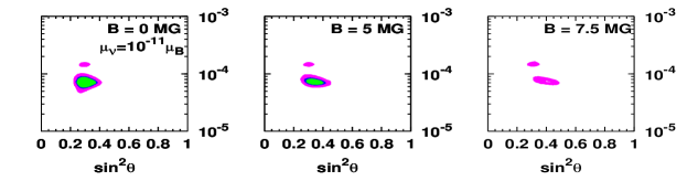
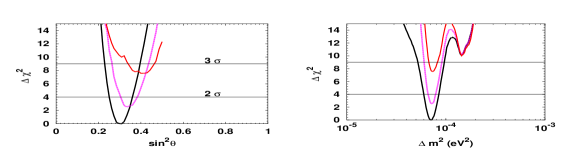
Figure 1: Solar neutrino oscillation parameters for zero (upper left panel) and non-zero (upper right panels) self-consistent CZ magnetic field used in Ref. Kutvitskii . Lower panels give $\Delta\chi^{2}$ profiles with respect to $\Delta m^{2}_{\textsc{sol}}$ and $\sin^{2}\theta_{\textsc{sol}}$.

We now turn to the recent KamLAND result on the $\bar{\nu_{e}}$ ’s from the Sun. The Collaboration has reported that the antineutrino flux $\Phi_{\bar{\nu_{e}}}$ is less than $3.7\times 10^{2}$ cm ^-2 s ^-1 at 90 % C. L. which corresponds to a 0.028 % of the solar ⁸ B $\nu_{e}$ flux (in the energy window between 8.3 MeV and 14.8 MeV). It is this last result that will substantially limit the possibility of subleading SFP component in the neutrino conversion mechanism, establishing the robustness of the oscillation hypothesis.

Within our generalized picture (LMA-MSW+SFP), after the MSW $\nu_{e}\to\nu_{\mu}$ conversion takes place in the central region of the Sun, $\bar{\nu_{e}}$’s are produced due to the magnetic moment conversion $\nu_{\mu}\to\bar{\nu_{e}}$. To analyse quantitatively the restrictions imposed by this result we consider three models for the solar magnetic field:

1. regular magnetic fields, both in the convective (CZ) Kutvitskii and radiative (RZ) Friedland zones of the Sun

2. convective zone random magnetic fields Bykov:1998gv

For definiteness we consider the simplest aproximate two-neutrino picture, which is justified in view of the stringent limits that follow mainly from reactor neutrino experiments Maltoni:2003da . From the resulting $4\times 4$ form of the neutrino evolution equation Schechter:1981hw ; Akhmedov:uk , we compute the expected $\bar{\nu_{e}}$ yield for each magnetic field model. For the case of CZ magnetic fields, this $4\times 4$ form of the neutrino evolution further decouples into LMA-MSW conversions deep in the Sun followed by (approximate) vacuum SFP conversions Schechter:1981hw inside the CZ. In contrast, for the RZ case there is no decoupling of the neutrino evolution, due to the large strength of the magnetic field .

In order to obtain a conservative bound on $\mu_{\nu}B$ we have calculated the minimum $\bar{\nu_{e}}$ yield as the oscillation parameters vary within the acceptable range (at the 90 % C.L.) in the absence of magnetic field (pure LMA-MSW case). Such minimum predicted anti-neutrino fluxes for the case of regular field profiles are shown in the curves depicted in Fig. 2, while the recent KamLAND limit is indicated by the lower horizontal lines. For comparison, we present the previous Super-K bound, indicated by the upper horizontal lines. Note that in both cases of regular field profile we can only constrain the product $\mu_{\nu}B$, as opposed to the intrinsic neutrino magnetic moment .  Grimus:2002vb .

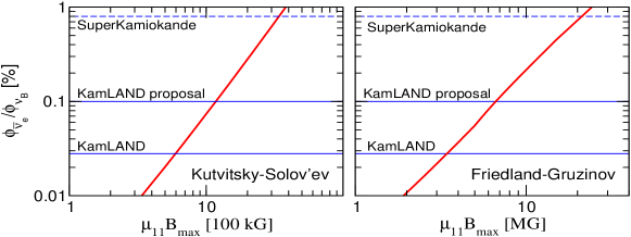
Figure 2: Bounds on $\mu_{\nu}B$ for regular magnetic field models, Kutvitsky-Solov’ev (left) and Friedland Gruzinov (right). The horizontal lines indicate the bounds on solar anti-neutrinos from Super-K and KamLAND.

A more interesting picture for SFP scenario is obtained if we consider the case of turbulent random magnetic fields inside the Sun. As we will see, the reason for this is twofold: (i) we will be able to fix, to some extent, the dependence on the magnetic field, in contrast to previous analysis of the random magnetic field presented in Ref. Bykov:1998gv ; Torrente-Lujan:1998sy , where an extra parameter $L_{0}$ appeared, characterizing the scale of the random magnetic field cells, and (ii) this model leads to more stringent limits on the neutrino magnetic moment by itself.

In the following we give a brief discussion of our new approach to the problem (a more detailed analysis will be published elsewhere Inprep ). The mean magnetic field value over the solar disc is of the order of 1 G and magnetic field strength in the solar spots reaches 1 kG. It is commonly accepted that fields measured at the solar surface are substantially weaker than those near the bottom of the convective zone (CZ) where they are supposed to be generated by a dynamo mechanism Yoshimura ; Sokoloff . In dynamo theory, the mean magnetic field is accompanied by a small-scale random magnetic field, which is not directly traced by sunspots or any other tracers of solar activity. By small scales we denote a typical scale of about the solar granule size ($\sim$ 1000 km) Stix where the rms magnetic field amplitudes (generated either as a by-product of a large-scale dynamo mechanism or directly by a small-scale dynamo) in the range of 50-100 kG are reasonable.

For LMA oscillations the MSW conversion occurs well below the CZ resulting in a coherent mixture of two neutrino flavours at the bottom of the convective zone. When neutrinos cross the randomly fluctuating magnetic field of the CZ it is expected that $\nu_{eL}$ will convert to ${\bar{\nu}_{\mu R}}$ and $\nu_{\mu L}$ will convert to $\bar{\nu}_{eR}$ as a result of the CZ magnetic field. For the case of random CZ magnetic fields these populations will tend to equilibrate. However, given the laboratory upper limits on $\mu_{\nu}$ and the finite depth of the CZ, this equilibration is not achieved. The relaxation can be viewed as a small-amplitude random walk of the neutrino polarization vector leading to a small appearance of electron and muon antineutrinos at the solar surface (cf. Loeb:1989dr for the vacuum case, and also discussion in Bykov:1998gv ). In what follows we describe the main features of this calculation and give the main result.

Because of the randomness of the underlying magnetic fields, the spin flavour evolution looses coherence, i.e., instead of evolving neutrino wave functions over the whole CZ and then obtaining the final probabilities, one has to compute the probabilities in each correlation cell and afterwards add them. As a result, independently of the random magnetic field model, the appearance of antineutrinos is proportional to the relevant Fourier harmonic of the transverse two-point magnetic correlation function, with space period equal to the LMA-MSW neutrino oscillation length (cf. Loeb:1989dr and discussion in Bamert:1997jj for the MSW matter noise).

We will assume for definiteness that random magnetic field evolution is due to the highly developed steady-state MHD turbulence treated within the Kolmogorov scaling theory Kolmogorov ; Landau . The magnetic Reynolds number within the CZ is very large, $R_{m}\sim 10^{8}$ Sokoloff , and the corresponding inertial range is very wide, $l_{\rm diss}<l<L_{\rm max}$ where the outer scale is supposed to be $L_{\rm max}\simeq 1000$ km, about the solar granule size, and   $l_{\rm diss}=L_{\rm max}R_{m}^{-3/4}\sim 1~{}$ m. The rms magnetic field $b_{l}$ is assumed to scale as $b_{l}\sim l^{1/3}$. This implies that, after fixing the maximum field amplitude at the outer scale $L_{\rm max}$ it is straightforward to obtain the rms field at the neutrino oscillation scale, which is about several hundreds kilometers for LMA-MSW case, well within the inertial range where scaling arguments are valid Inprep . Here we show only the final result for neutrino mass eigenstate probabilities at the surface of the Sun:

$$|\nu_{1L}|^{2}_{R_{\odot}}=P_{1}(1-\eta),\qquad|\nu_{2R}|^{2}_{R_{\odot}}=P_{1}\eta~{},$$ (1)

$$|\nu_{2L}|^{2}_{R_{\odot}}=P_{2}(1-\eta),\qquad|\nu_{1R}|^{2}_{R_{\odot}}=P_{2}\eta~{},$$ (2)

(note that these obey unitarity) where the common factor $\eta$ is given by

$$\eta\simeq 0.3~{}\frac{{\mu_{\nu}}^{2}\bar{b}_{\rm max}^{2}}{{\delta^{2}}}\frac{\delta\cdot L}{(\delta\cdot L_{\rm{max}})^{2/3}}S^{2}~{}.$$ (3)

Here $P_{i}=P_{iL}=|\nu_{iL}(r=0.7R_{\odot})|^{2}$ are the probabilities that solar neutrinos reach the bottom of the CZ in a given mass state, $L$ is the CZ width, $\delta=\Delta m^{2}/4E$, and $S^{2}$ is a rms magnetic field profile shape factor

$$S^{2}=\frac{1}{L}\int_{0}^{L}dz\frac{{\bar{b}^{2}}(z)}{{\bar{b}_{max}}^{2}}.$$ (4)

Note that $S=1$ for constant shape of rms field and of the order of unity for other profiles, e.g. $S=0.579$ for the “smooth” profile of Bykov:1998gv , and $S=0.577$ for a triangle profile.

The different factors in Eq. 3 can be explained if we keep in mind that $\delta$ is inversely proportional to the neutrino oscillation length, $\delta=\pi/\lambda_{osc}$ . The ratio $\bar{b}_{\rm max}^{2}/(\delta\cdot L_{\rm{max}})^{2/3}=\bar{b}_{\lambda_{\rm osc}}^{2}$ is the squared rms field at the scale $l=1/\delta\sim\lambda_{\rm osc}$, and the ratio $\mu^{2}_{\nu}\bar{b}_{\lambda_{\rm osc}}^{2}/\delta^{2}$ determines the fraction of neutrinos which experience (on average) spin-flavour conversion to the antineutrino states in a correlation cell of length $l\sim\lambda_{\rm osc}$. Finally $\delta\cdot L\sim L/\lambda_{\rm osc}$ is the number of correlation cells along the neutrino trajectory and the factor $S^{2}$, as already mentioned, accounts for the specific shape of the rms field profile. (The numerical factor 0.3 comes from the integration along the trajectory).

We can rewrite Eq. 3 in normalized units as

$$\eta\sim 3\times 10^{-3}\mu_{11}^{2}\varepsilon^{2}S^{2}\left(\frac{7\times 10^{-5}eV^{2}}{\Delta m^{2}}\right)^{5/3}\left(\frac{E}{10{\rm MeV}}\right)^{5/3}$$ (5)

where $\mu_{11}$ is the magnetic moment in units of $10^{-11}\mu_{B}$, and the ratio $\varepsilon=(b/100~{}{\rm kG})(L_{{\rm max}}/1000~{}{\rm km})^{1/3}$.

Although the ratio $\varepsilon$ is not known precisely, we can obtain a good estimate assuming the equipartition between kinetic energy of hydrodynamic pulsations and the rms magnetic energy at the upper (most energetic) scale $L_{max}$ Sokoloff

$$\frac{\rho\bar{v^{2}}}{2}\sim\frac{\bar{b}_{\rm max}^{2}}{8\pi}$$ (6)

Taking $v\sim 3\times 10^{4}{\rm cm}/{\rm s}$, $\rho\sim 1g/{\rm cm}^{3}$ we obtain $b_{\rm max}\sim 100$ kG. In what follows we will consider the range $b_{\rm max}\sim 50-100$ kG.

This specific behaviour implies, on physical grounds, that $\varepsilon$ is not allowed to vary substantially, $0.5<\varepsilon<1$, with our assumptions. As mentioned, for different profiles we found that the parameter $S^{2}$ lies in the range between 0.5 and 1. With this in mind, we can see that the product $k=\varepsilon S$ lies in the interval $0.25<k<1$. Since the overall $\nu_{e}\to\bar{\nu_{e}}$ conversion probability depends linearly on $\eta$, it follows that, by comparing the resulting $\bar{\nu_{e}}$ yield to the recent KamLAND bound one can constrain the value of $\mu_{\nu}$ to within a factor 4. More precisely, we have computed the solar anti-neutrino yield for this random magnetic field model for all allowed values of neutrino oscillation parameters in the LMA-MSW region. Our results are shown in fig. 3 as a function of $\mu_{\nu}$, where the width of the band corresponds to the freedom in choosing the parameter $k$. It is easy to see that, indeed, the constraint we obtain is better than those that hold for the case of regular magnetic fields. Moreover, from our estimate for the minimum value of $k$, we can obtain an upper bound for $\mu_{\nu}$ which lies in the range $\mu_{\nu}\leq 1.5\times 10^{-12}\mu_{B}$ to $\mu_{\nu}\leq 5\times 10^{-12}\mu_{B}$.

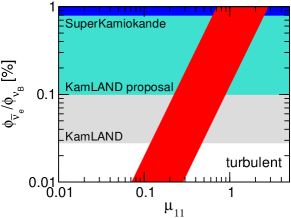
Figure 3: Bounds on $\mu_{\nu}$ for the turbulent magnetic field model described in the text. The horizontal lines indicate the bounds on solar anti-neutrinos from Super-K and KamLAND.

We have obtained this result for the Kolmogorov theory. However, it can be easily generalized for arbitrary power-law exponent $p$ (for Kolmogorov theory $p=5/3$). We have checked that our bound on $\mu_{\nu}$ is rather robust with respect to possible changes of the power-law exponent $p$ within the interval from 1 to 2 Inprep .

In short, we have discussed the impact of recent solar neutrino data on the spin-flavor-precession (SFP) mechanism of neutrino conversion. The recent KamLAND bound on the solar anti-neutrino yield leads to a constraint on the product of Majorana neutrino transition magnetic moment and some magnetic field strength in different models for the solar magnetic field. For the case of random magnetic fields inside the Sun, one can obtain a direct constraint on the intrinsic neutrino magnetic moment of $\mu_{\nu}\mathrel{\raise 1.29167pt\hbox{$<$\kern-7.5pt\lower 4.30554pt\hbox{$\sim$}}}{\rm few}\times 10^{-12}\mu_{B}$, similar to bounds obtained from star cooling. Comparing these constraints with Fig. 1 one sees that the robustness of the oscillation interpretation of current solar neutrino data against possible magnetic-field-induced transitions is firmly established.

We thank V. B. Semikoz and D. D. Sokoloff for useful discussions. This work was supported by Spanish grant BFM2002-00345, by European RTN network HPRN-CT-2000-00148, by European Science Foundation network grant N. 86, by INTAS YSF grant 2001/2-148 and MECD grant SB2000-0464 (TIR). TIR and AIR were partially supported by the Presidium RAS and CSIC-RAS grants. OGM was supported by CONACyT-Mexico and SNI.

References

- (1) [KamLAND Collaboration], Phys. Rev. Lett. 92 071301 (2004) 071301.
- (2) [KamLAND Collaboration], Proposal for US participation in KamLAND, 1999.
- (3) Y. Gando et al. [Super-Kamiokande Collaboration], Phys. Rev. Lett. 90, 171302 (2003) [hep-ex/0212067].
- (4) J. Schechter and J. W. F. Valle, Phys. Rev. D 24, 1883 (1981) [Erratum-ibid. D 25, 283 (1982)].
- (5) E. K. Akhmedov, Phys. Lett. B 213, 64 (1988); C. S. Lim and W. J. Marciano, Phys. Rev. D 37, 1368 (1988).
- (6) J. Schechter and J. W. F. Valle, Phys. Rev. D 25, 774 (1982); G. B. Gelmini and J. W. F. Valle, Phys. Lett. B 142, 181 (1984); M. C. Gonzalez-Garcia and J. W. F. Valle, Phys. Lett. B 216, 360 (1989); J. F. Beacom and N. F. Bell, Phys. Rev. D 65, 113009 (2002) [arXiv:hep-ph/0204111].
- (7) V. A. Kutvitskii, L. Solov’ev JETP 78 456 (1994)
- (8) E. K. Akhmedov, J. Pulido, Phys. Lett. B 553, 7 (2003); M. Guzzo, H. Nunokawa, Astropart. Phys. 12, 87 (1999)
- (9) A. Friedland and A. Gruzinov, Astropart. Phys. 19, 575 (2003)
- (10) K. Eguchi et al.,Phys. Rev. Lett. 90, 021802 (2003).
- (11) J. Barranco et al, Phys. Rev. D 66, 093009 (2002), see version v3 of hep-ph/0207326 for KamLAND update.
- (12) S. N. Ahmed et al.,Phys. Rev. Lett. 92 181301 (2004).
- (13) M. Maltoni et al., Phys. Rev. D 68 (2003) 113010. For pre-salt, post-KamLAND analyses see M. Maltoni, T. Schwetz, and J. W. F. Valle, Phys. Rev. D 67, 093003 (2003) and references therein.
- (14) O. G. Miranda et al, Nucl. Phys. B 595, 360 (2001); Phys. Lett. B 521, 299 (2001).
- (15) W. Grimus et al, Nucl. Phys. B 648, 376 (2003)
- (16) Z. Daraktchieva et al., Phys. Lett. B 564, 190 (2003); J. F. Beacom and P. Vogel, Phys. Rev. Lett. 83, 5222 (1999)
- (17) F. Moreno-Insertis, Astron.& Astrophys. 166, 291 (1986).
- (18) A. A. Bykov, V. Y. Popov, A. I. Rez, V. B. Semikoz and D. D. Sokoloff, Phys. Rev. D 59, 063001 (1999).
- (19) E. Torrente-Lujan, Phys. Rev. D 59 (1999) 093006; V. B. Semikoz and E. Torrente-Lujan, Nucl. Phys. B 556 (1999) 353 P. Aliani et al., JHEP 0302 (2003) 025; E. Torrente-Lujan, JHEP 0304 (2003) 054
- (20) O. G. Miranda et al, in preparation.
- (21) H. Yoshimura, Astrophys. J., 178 (1972) 863; Astrophys. J. Suppl. Ser., 52 (1983) 363; M. Stix, Astron. & Astrophys. 47 (1976) 243.
- (22) Ya. B. Zeldovich, A. A. Ruzmaikin and D.D. Sokoloff, Magnetic Fields in Astrophysics, Gordon and Breach Science Publishers, 1983 and references therein.
- (23) M. Stix, The Sun: An Introduction (Astronomy and Astrophysics Library), Springer Verlag 1991.
- (24) A. Loeb and L. Stodolsky, Phys. Rev. D 40, 3520 (1989).
- (25) P. Bamert, C. P. Burgess and D. Michaud, Nucl. Phys. B 513, 319 (1998) [arXiv:hep-ph/9707542].
- (26) A. Kolmogorov, Dokl. Akad. Nauk. SSSR 31, 538 (1941); 32, 19 (1941); [Proc. R. Soc. London] A 434 15 (1991).
- (27) L. D. Landau and E. M. Lifshitz, Fluid Mechanics, Pergamon 1984.