Direct CP violation and new physics effects

in the decay mode $B^{+}\rightarrow\phi K^{+}$

Anjan K. Giri1 and Rukmani Mohanta2 1 Physics Department, Technion-Israel Institute of Technology, 32000 Haifa, Israel
2 School of Physics, University of Hyderabad, Hyderabad - 500046, India


()

Abstract

We study the direct CP violation effect in the decay mode $B^{+}\to\phi K^{+}$. This decay mode is dominated by the loop induced $\bar{b}\to\bar{s}s\bar{s}$ penguin diagram with a tiny contribution from the annihilation diagram. Therefore, the standard model expectation of direct CP violation is negligibly small. Using QCD factorization approach we find the CP asymmetry in the standard model to be at percent level. We consider then two scenarios beyond the standard model, the model with an extra vector-like down quark (VLDQ) and the R-parity violating supersymmetric model (RPV) and show that the direct CP violating asymmetry in $B^{+}\to\phi K^{+}$ could be as large as $\sim 85\%$ ($70\%$) in VLDQ (RPV) model.

1 Introduction

The study of $B$ physics and CP violation is now at the center stage of high energy physics research with dedicated $B$ factories (BABAR and Belle) already having an accumulation of huge data in the $B$ sector. With these two $B$ factories in full operation and hadronic machines coming up, the flavor sector of the standard model (SM) will be subjected to stringent tests in the near future. The major goal of these $B$ factories is not only to test the predictions of the SM but also to reveal the presence of new physics (NP), if any. CP violation in $B$ system has been confirmed recently at both the $B$ factories with the measurement of $\sin 2\beta$ (where $\beta$ is one of the angles of CKM unitarity triangle) in the $B^{0}\to\psi K_{S}$ decay [1]. It should be emphasized here that the current measured value of $(\sin 2\beta)_{\psi K_{S}}$ by both the $B$ factories are very close to each other [2]. The present world avarage on $(\sin 2\beta)_{\psi K_{S}}$ [2] is

$$\sin(2\beta)_{\psi K_{S}}=0.736\pm 0.049\;,$$ (1)

which is in very good agreement with the SM expectation. However, this result does not exclude intersting CP violating new physics effects in other $B$ decays. The rare decay mode $B^{0}\to\phi K_{S}$, which is a pure penguin process, involving the quark level transition $b\to s\bar{s}s$, is one of the channels which provides powerful testing ground for new physics. The reason is very simple because in the SM the direct decay amplitudes for $B^{0}\to\psi K_{S}$ and $B^{0}\to\phi K_{S}$ modes have vanishing weak phase (in the Wolfenstein parametrization). Thus, the time dependent mixing-induced CP asymmetry in both decays is due to the weak phase in $B^{0}-\bar{B}^{0}$ mixing and expected to give the same value, i.e., $\sin 2\beta$. In the SM, the difference between these two measurements is expected to be very small [3]

|sin(2Ξ²)Οˆβ€‹KSβˆ’sin(2Ξ²)ϕ​KS| < ∼ π’ͺ(Ξ»2),|\sin(2\beta)_{\psi K_{S}}-\sin(2\beta)_{\phi K_{S}}|\mathrel{\vbox{\hbox{$<$}\nointerlineskip\hbox{$\sim$}}}{\cal O}(\lambda^{2})\;, (2)

with $\lambda\sim 0.22$. However, the recent measurements of sin 2$\beta$ in the $B^{0}\to\phi K_{S}$ decay at BABAR and Belle give the average value [2]

$$\sin(2\beta)_{\phi K_{S}}=-0.15\pm 0.33\;,$$ (3)

which is about $2.7\sigma$ deviation away from the corresponding measurement of $(\sin 2\beta)_{\psi K_{S}}$. The discrepancy between the measured values of $(\sin 2\beta)_{\psi K_{S}}$ and $(\sin 2\beta)_{\phi K_{S}}$ may imply the possible existence of new physics in one of the decay modes.

If there is new physics, then it could affect the $B^{0}-\bar{B}^{0}$ mixing as well as the decay amplitudes. But the NP contribution arising from mixing, will be same (i.e., universal) in both the processes . So when we compare the measurements of $\sin 2\beta$ in both the two decays then the NP contribution, if any in mixing, will not appear in the comparison, since it will affect both the decays with the same amount. Whereas, the NP contribution present in the decay amplitudes are nonuniversal and process dependent and can vary from process to process. The striking difference between these two decays is that $B^{0}\to\psi K_{S}$ is a tree level ($b\to c\bar{c}s$) process whereas $B^{0}\to\phi K_{S}$ is a purely loop induced penguin process. So the NP contribution to $B^{0}\to\psi K_{S}$ is expected to be suppressed and it could be significant for the loop induced process $B^{0}\to\phi K_{S}$. So, the discrepancy between the measured values of $(\sin 2\beta)_{\psi K_{S}}$ and $(\sin 2\beta)_{\phi K_{S}}$ may indicate the possibility of NP effect in the decay amplitude of $B^{0}\to\phi K_{S}$.

Recently, various new physics scenarios have been explored to explain the above discrepancy [4, 5, 6, 7]. If new physics effects indeed are present in the decay mode $B^{0}\to\phi K_{S}$, then one can expect to observe similar effects in other modes having the same internal quark structure. It is therefore important to explore other signals of new physics in order to corroborate this result. One way to search for new physics effects is to look for direct CP violation in the decay modes which are having a single decay amplitude in the standard model and hence expected to give zero direct CP asymmetry. An observation of nonzero direct CP violation in such modes is an unambiguous signal of new physics.

At present, it appears from the current trend of data that new physics effects might be present in the $B^{0}\to\phi K_{S}$ mode. It is therefore interesting to see the effects of NP in the penguin dominated decay mode $B^{\pm}\to\phi K^{\pm}$ also (which is having the same underlying quark dynamics) alongwith a tiny annihilation contribution, which is our prime objective in this paper. The branching ratio and CP asymmetry measurements for this mode have recently been reported by both the Belle [8], BABAR [9] and CLEO [10] collaborations, which are given below as

$\displaystyle{\rm Br}(B^{+}\to\phi K^{+})$ $\displaystyle=$ $\displaystyle(9.4\pm 1.1\pm 0.7)\times 10^{-6}~{}~{}~{}~{}~{}~{}~{}~{}~{}{\rm Belle}\;,$
$\displaystyle{\cal A}_{\rm CP}(B^{+}\to\phi K^{+})$ $\displaystyle=$ $\displaystyle 0.01\pm 0.12\pm 0.05~{}~{}~{}~{}~{}~{}~{}~{}~{}~{}~{}~{}~{}~{}~{}~{}{\rm Belle}\;,$
$\displaystyle{\rm Br}(B^{+}\to\phi K^{+})$ $\displaystyle=$ $\displaystyle(10.0^{+0.9}_{-0.8}\pm 0.5)\times 10^{-6}~{}~{}~{}~{}~{}~{}~{}~{}~{}~{}{\rm BABAR}\;,$
$\displaystyle{\cal A}_{\rm CP}(B^{+}\to\phi K^{+})$ $\displaystyle=$ $\displaystyle 0.04\pm 0.09\pm 0.01~{}~{}~{}~{}~{}~{}~{}~{}~{}~{}~{}~{}~{}~{}~{}~{}{\rm BABAR}\;,$
$\displaystyle{\rm Br}(B^{+}\to\phi K^{+})$ $\displaystyle=$ $\displaystyle(5.5^{+2.1}_{-1.8}\pm 0.6)\times 10^{-6}~{}~{}~{}~{}~{}~{}~{}~{}~{}~{}~{}~{}{\rm CLEO}\;.$ (4)

The average branching ratio and CP asymmetry are given as

$\displaystyle{\rm Br}(B^{+}\to\phi K^{+})$ $\displaystyle=$ $\displaystyle(9.2\pm 0.7)\times 10^{-6}\;,$
$\displaystyle{\cal A}_{\rm CP}(B^{+}\to\phi K^{+})$ $\displaystyle=$ $\displaystyle 0.03\pm 0.07\;.$ (5)

At this point we ask the question whether the possibility of NP effect in the decay mode $B^{+}\to\phi K^{+}$ has already been ruled out ? In the rest of the paper our objective will be to closely examine this question and try to obtain a meaningful answer, if any. If one looks at the data on the direct CP asymmetry, then certainly nothing can be concluded at present. That is the central value is higher than the SM expectation, but as error bars are also significantly large, one simply cannot conclude/exclude the possibility of NP effect. So the present status is that, it is premature to say anything and to be more precise, on which side (i.e., within or outside) of the SM they are, as far as direct CP violation in $B^{\pm}\to\phi K^{\pm}$ is concerned. To summarize, although the CP violating asymmetry is not very much larger than the SM expected value, but due to the presence of large error bars, decisive conclusion regarding the presence/absence of NP effect cannot be inferred.

This in turn gives us enough room to explore NP effect. In fact if in future the data stabilize with even a few percent of direct CP asymmetry, then it may be very hard to explain the same under the framework of the SM and eventually that may lead to the establishment of NP in this mode. Keeping this in mind we now study carefully to find the answer to our question that we raised earlier.

In this paper, we intend to study the direct CP violation effects in the decay mode $B^{\pm}\to\phi K^{\pm}$. We use the QCD factorization method [11, 12] to evaluate the relevant branching ratio and the direct CP asymmetry ${\cal A}_{\rm CP}$, in the SM. This decay mode $B^{\pm}\to\phi K^{\pm}$ has recently been studied in the SM using QCD factorization [13, 14, 15]. However, the predicted branching ratio found to be well below the present experimental value. Next, we consider two beyond the standard model scenarios, the so called R-parity violating supersymmetric model and the model with an extra vector-like down quark. These two models were explored recently to explain the observed discrepancy in $B^{0}\to\phi K_{S}$ mode [5, 6, 7].

The paper is organized as follows. Section II includes a general description of CP violating parameter in $B^{\pm}\to\phi K^{\pm}$ decays, while in Sect. III we analyze the decay mode $B^{\pm}\to\phi K^{\pm}$ in the SM using the QCD factorization. The new physics effects from the VLDQ model and the RPV model are considered in sections IV and V respectively and in Section Β VI we present some concluding remarks.

2 CP violating Asymmetry

Here we briefly present the basic and well known formula for the CP violating asymmetry parameter. For charged $B^{\pm}\to\phi K^{\pm}$ decays the CP violating rate asymmetries in the partial rates are defined as follows :

$${\cal A}_{\rm CP}=\frac{\Gamma(B^{-}\to\phi K^{-})-\Gamma(B^{+}\to\phi K^{+})}{\Gamma(B^{-}\to\phi K^{-})+\Gamma(B^{+}\to\phi K^{+})}\;.$$ (6)

Without loss of generality we can write the decay amplitudes as

$\displaystyle A(B^{-}\to\phi K^{-})$ $\displaystyle=$ $\displaystyle\lambda_{u}|A_{u}|e^{i\delta_{u}}+\lambda_{c}|A_{c}|e^{i\delta_{c}}\;,$
$\displaystyle A(B^{+}\to\phi K^{+})$ $\displaystyle=$ $\displaystyle\lambda_{u}^{*}|A_{u}|e^{i\delta_{u}}+\lambda_{c}^{*}|A_{c}|e^{i\delta_{c}}\;,$ (7)

where Ξ»q=Vq​b​Vq​sβˆ—subscriptπœ†π‘žsubscriptπ‘‰π‘žπ‘superscriptsubscriptπ‘‰π‘žπ‘ \lambda_{q}=V_{qb}V_{qs}^{*}, $A_{u}$ and $A_{c}$ denote the contributions arising from the current operators proportional to the product of CKM matrix elements $\lambda_{u}$ and $\lambda_{c}$ respectively. The corresponding strong phases are denoted by $\delta_{u}$ and $\delta_{c}$. Thus the CP violating asymmetry is given as

$\displaystyle{\cal A}_{\rm CP}$ $\displaystyle=$ $\displaystyle\frac{-2{\rm Im}(\lambda_{u}\lambda_{c}^{*}){\rm Im}(A_{u}A_{c}^{*})}{|\lambda_{u}A_{u}|^{2}+|\lambda_{c}A_{c}|^{2}+2{\rm Re}(\lambda_{u}\lambda_{c}^{*}){\rm Re}(A_{u}A_{c}^{*})}$ (8)
$\displaystyle=$ $\displaystyle\frac{2\sin\gamma\sin(\delta_{u}-\delta_{c})}{|\frac{\lambda_{u}A_{u}}{\lambda_{c}A_{c}}|+|\frac{\lambda_{c}A_{c}}{\lambda_{u}A_{u}}|+2\cos\gamma\cos(\delta_{u}-\delta_{c})}\;,$

where $-\gamma$ is the weak phase of $\lambda_{u}$, and $\lambda_{c}$ is real in the Wolfenstein parametrization. Thus to obtain significant direct CP asymmetry, one requires the two interfering amplitudes to be of same order and their relative strong phase should be significantly large (i.e., close to $\pi/2$). However, in the SM, the ratio of the CKM matrix elements of the two terms in Eq. (7) can be given (in the Wolfenstein parametrization) as $|\lambda_{u}/\lambda_{c}|\simeq\lambda^{2}\sqrt{\rho^{2}+\eta^{2}}\simeq 2\%$. Therefore, the first amplitude will be highly suppressed with respect to the second unless $A_{u}>>A_{c}$. Therefore, the naive SM expectation on ${\cal A}_{\rm CP}$ is that it is negligibly small. This in turn makes the mode interesting to look for the NP in terms of large direct CP asymmetry.

In the presence of new physics the amplitude can be written as

$$A(B^{-}\to\phi K^{-})=A_{SM}+A_{NP}=A_{SM}\left[1+r_{NP}~{}e^{i\phi_{NP}}\right]\;,$$ (9)

where $r_{NP}=|A_{NP}/A_{SM}|$, ($A_{SM}$ and $A_{NP}$ correspond to the SM and NP contributions to the $B^{-}\to\phi K^{-}$ decay amplitude respectively) and $\phi_{NP}={\rm arg}(A_{NP}/A_{SM})$, which contains both strong and weak phase components. The branching ratio for the $B^{-}\to\phi K^{-}$ decay process can be given as

$${\rm Br}(B^{-}\to\phi K^{-})={\rm Br^{SM}}\left(1+r_{NP}^{2}+2r_{NP}\cos\phi_{NP}\right)\;,$$ (10)

where ${\rm Br^{SM}}$ represents the corresponding standard model value.

To find out the CP asymmetry, it is necessary to represent explicitly the strong and weak phases of the SM as well as NP amplitudes. Although, it is expected that the SM amplitude $\lambda_{u}A_{u}$ is highly suppressed with respect to its $\lambda_{c}A_{c}$ counterpart, for completeness we will keep this term for the evaluation of ${\cal A}_{\rm CP}$. We denote the NP contribution to the decay amplitude as $A_{NP}=|A_{NP}|e^{i(\delta_{n}+\theta_{n})}$, where $\delta_{n}$ and $\theta_{n}$ denote the strong and weak phases of the NP amplitude respectively. Thus, in the presence of NP, we can explicitly write the decay amplitude for $B^{-}\to\phi K^{-}$ mode as

$$A(B^{-}\to\phi K^{-})=\lambda_{u}|A_{u}|e^{i\delta_{u}}+\lambda_{c}|A_{c}|e^{i\delta_{c}}+|A_{NP}|e^{i(\delta_{n}+\theta_{n})}\;.$$ (11)

The amplitude for $B^{+}\to\phi K^{+}$ mode is obtained by changing the sign of the weak phases of the amplitude (11). Thus, the CP asymmetry parameter (6) is given as

$${\cal A}_{\rm CP}=\frac{2\biggr{(}|\lambda_{u}\lambda_{c}A_{u}A_{c}|\sin\gamma\sin\delta_{uc}+|\lambda_{u}A_{u}A_{NP}|\sin(\gamma+\theta_{n})\sin\delta_{un}+|\lambda_{c}A_{c}A_{NP}|\sin\theta_{n}\sin\delta_{cn}\biggr{)}}{|{\cal A}|^{2}+2\biggr{\{}|\lambda_{u}A_{u}|\biggr{(}|\lambda_{c}A_{c}|\cos\gamma\cos\delta_{uc}+|A_{NP}|\cos(\gamma+\theta_{n})\cos\delta_{un}\biggr{)}+|\lambda_{c}A_{c}A_{NP}|\cos\theta_{n}\cos\delta_{cn}\biggr{\}}},$$ (12)

where $|{\cal A}|^{2}=(|\lambda_{u}A_{u}|^{2}+|\lambda_{c}A_{c}|^{2}+|A_{NP}|^{2})$ and $\delta_{ij}=\delta_{i}-\delta_{j}$ are the relative strong phases between different amplitudes. If we neglect the $\lambda_{u}A_{u}$ component in the decay amplitude (11), the CP asymmetry will be reduced to

$${\cal A}_{\rm CP}=\frac{2\biggr{(}|\lambda_{c}A_{c}A_{NP}|\sin\theta_{n}\sin(\delta_{c}-\delta_{n})\biggr{)}}{|\lambda_{c}A_{c}|^{2}+|A_{NP}|^{2}+2\biggr{(}|\lambda_{c}A_{c}A_{NP}|\cos\theta_{n}\cos(\delta_{c}-\delta_{n})\biggr{)}}.$$ (13)

Having obtained the direct CP asymmetry parameter ${\cal A}_{\rm CP}$ in the presence of new physics we now proceed to evaluate the same within and beyond the SM, in the following sections.

3 CP Violation in $B^{\pm}\to\phi K^{\pm}$ process in the SM

To study the CP violation effects in $B^{\pm}\to\phi K^{\pm}$ process, first we present the SM amplitude and find out the branching ratio and CP asymmetry parameter. In the SM, the decay process $B^{\pm}\to\phi K^{\pm}$ receives dominant contribution from the quark level transition $b\to s\bar{s}s$, which is induced by the QCD, electroweak and magnetic penguins and a tiny annihilation contribution. The effective $\Delta B=\Delta S=1$ Hamiltonian relevant for the process under consideration is given as [11]

$$H_{eff}=\frac{G_{F}}{\sqrt{2}}\biggr{[}V_{ub}V_{us}^{*}\sum_{i=1}^{2}C_{i}O_{i}+V_{qb}V_{qs}^{*}\sum_{j=3}^{11}C_{j}O_{j}\biggr{]},$$ (14)

where $q=u,~{}c$. $O_{1,2}$, $O_{3},\cdots,O_{6}$ and $O_{7},\cdots,O_{10}$ are the standard model tree, QCD and EW penguin operators, respectively, and $O_{11}$ is the gluonic magnetic operator. The values of the Wilson coefficients at the scale $\mu\approx m_{b}$ in the NDR scheme are given in Ref. [16] as

$\displaystyle C_{1}=1.082\;,~{}~{}~{}~{}C_{2}=-0.185\;,~{}~{}~{}~{}C_{3}=0.014\;,~{}~{}~{}~{}~{}~{}C_{4}=-0.035\;,$
$\displaystyle C_{5}=0.009\;,~{}~{}~{}~{}C_{6}=-0.041\;,~{}~{}~{}~{}C_{7}=-0.002\alpha\;,~{}~{}~{}C_{8}=0.054\alpha\;,$
$\displaystyle C_{9}=-1.292\alpha\;,~{}~{}~{}~{}C_{10}=0.263\alpha\;,~{}~{}~{}~{}C_{11}=0.052\;.$ (15)

We use QCD factorization [11, 12] to evaluate the hadronic matrix elements. In this method, the decay amplitude can be represented in the form

$$\langle\phi K^{-}|O_{i}|B^{-}\rangle=\langle\phi K^{-}|O_{i}|B^{-}\rangle_{\rm fact}\biggr{[}1+\sum r_{n}\alpha_{s}^{n}+{\cal O}(\Lambda_{\rm QCD}/m_{b})\biggr{]}\;,$$ (16)

where $\langle\phi K^{-}|O_{i}|B^{-}\rangle_{\rm fact}$ denotes the naive factorization result and $\Lambda_{\rm QCD}\sim 225$ MeV, the strong interaction scale. The second and third terms in the square bracket represent higher order $\alpha_{s}$ and $\Lambda_{\rm QCD}/m_{b}$ corrections to hadronic matrix elements. We shall closely follow the approaches [13, 14, 15, 17] to reanalyze our QCD factorization calculation. In a recent paper Beneke and Neubert have presented the latest QCD factorization calculation [18], where the authors have considered 4 different schemes to find a suitable set of parameters which can explain the observed data. Furthermore, it has been shown in that paper that the last scheme, i.e., S4 (scheme 4) explains the observed data on branching ratios and CP violation parameters to a good accuracy. Of course it should be mentioned here that even the scheme S4 also fails to explain the problematic penguin dominated $B\to\phi K$ modes [18, 19].

In this analysis, however, we will restrict ourselves to the default QCD factorization (by default we mean the QCD factorization result without any parameter readjustment (for more details the reader is referred to Ref. [18]). This is done so, because of the fact that one should not just ignore the possibility of NP effect. Furthermore, we do not see why the parameter readjustment is the only possibility to match the data (eventhough it may be a logistic option and in the long run may even come out to be true). So, in order to visualize the NP effect, we confine ourselves to the default values of the QCD factorization and allow NP to fill up the gap between the experimental data and the SM values rather than readjusting the parameters to find a good agreement. In doing so, we can accommodate the beyond the SM scenarios, if any, to explain the possible discrepancy. Nevertheless, we will compare the results of Ref. [18] wherever necessary to that of our work. It should be emphasized here that our speculation regarding the presence of NP may not be unrealistic. As a matter of fact the present data in this sector do not seem to comply with the SM expectations, already mentioned earlier, as in the case of $B^{0}\to\phi K_{S}$ decay.

In the heavy quark limit the decay amplitude for the $B^{-}\to\phi K^{-}$ process, arising from the penguin diagrams, is given as

$\displaystyle A^{P}(B^{-}\to\phi K^{-})=\frac{G_{F}}{\sqrt{2}}\sum_{q=u,~{}c}V_{qb}V_{qs}^{*}\biggr{[}a_{3}^{q}+a_{4}^{q}+a_{5}^{q}-\frac{1}{2}\left(a_{7}^{q}+a_{9}^{q}+a_{10}^{q}\right)+a_{10a}^{q}\biggr{]}X\;,$ (17)

where $X$ is the factorized matrix element. Using the form factors and decay constants defined as [20]

$\displaystyle\langle K^{-}(p_{K})|\bar{s}\gamma^{\mu}b|B^{-}(p_{B})\rangle$ $\displaystyle=$ $\displaystyle\biggr{[}(p_{B}+p_{K})^{\mu}-\frac{m_{B}^{2}-m_{K}^{2}}{q^{2}}q^{\mu}\biggr{]}F_{1}(q^{2})$
$\displaystyle+$ $\displaystyle\frac{m_{B}^{2}-m_{K}^{2}}{q^{2}}q^{\mu}F_{0}(q^{2})\;,$
βŸ¨Ο•β€‹(q,Ο΅)|s¯​γμ​s|0⟩quantum-operator-productitalic-Ο•π‘žitalic-ϡ¯𝑠superscriptπ›Ύπœ‡π‘ 0\displaystyle\langle\phi(q,\epsilon)|\bar{s}\gamma^{\mu}s|0\rangle $\displaystyle=$ $\displaystyle f_{\phi}~{}m_{\phi}~{}\epsilon^{\mu}\;,$ (18)

we obtain

$\displaystyle X$ $\displaystyle=$ $\displaystyle\langle K^{-}(p_{K})|\bar{s}\gamma_{\mu}(1-\gamma_{5})b|B^{-}(p_{B})\rangle\langle\phi(q,\epsilon)|\bar{s}\gamma^{\mu}(1-\gamma_{5})s|0\rangle$ (19)
$\displaystyle=$ $\displaystyle 2F^{B\to K}_{1}(m_{\phi}^{2})~{}f_{\phi}~{}m_{\phi}~{}(\epsilon\cdot p_{B})\;.$

The coefficients $a_{i}^{q}$’s which contain next to leading order (NLO) and hard scattering corrections are given as [13, 17]

$\displaystyle a_{3}^{u}$ $\displaystyle=$ $\displaystyle a_{3}^{c}~{}=~{}C_{3}+\frac{C_{4}}{N}+\frac{\alpha_{s}}{4\pi}\frac{C_{F}}{N}C_{4}F_{\phi}\;,$
$\displaystyle a_{4}^{q}$ $\displaystyle=$ $\displaystyle C_{4}+\frac{C_{3}}{N}+\frac{\alpha_{s}}{4\pi}\frac{C_{F}}{N}\biggr{[}C_{3}\left[F_{\phi}+G_{\phi}(s_{s})+G_{\phi}(s_{b})\right]\;,$
$\displaystyle+$ $\displaystyle C_{1}G_{\phi}(s_{q})+(C_{4}+C_{6})\sum_{f=u}^{b}G_{\phi}(s_{f})+C_{11}G_{\phi,11}\biggr{]}\;,$
$\displaystyle a_{5}^{u}$ $\displaystyle=$ $\displaystyle a_{5}^{c}~{}=~{}C_{5}+\frac{C_{6}}{N}+\frac{\alpha_{s}}{4\pi}\frac{C_{F}}{N}C_{6}(-F_{\phi}-12)\;,$
$\displaystyle a_{7}^{u}$ $\displaystyle=$ $\displaystyle a_{7}^{c}~{}=~{}C_{7}+\frac{C_{8}}{N}+\frac{\alpha_{s}}{4\pi}\frac{C_{F}}{N}C_{8}(-F_{\phi}-12)\;,$
$\displaystyle a_{9}^{u}$ $\displaystyle=$ $\displaystyle a_{9}^{c}~{}=~{}C_{9}+\frac{C_{10}}{N}+\frac{\alpha_{s}}{4\pi}\frac{C_{F}}{N}C_{10}F_{\phi}\;,$
$\displaystyle a_{10}^{u}$ $\displaystyle=$ $\displaystyle a_{10}^{c}~{}=~{}C_{10}+\frac{C_{9}}{N}+\frac{\alpha_{s}}{4\pi}\frac{C_{F}}{N}C_{9}F_{\phi}\;,$
$\displaystyle a_{10a}^{q}$ $\displaystyle=$ $\displaystyle\frac{\alpha_{s}}{4\pi}\frac{C_{F}}{N}\biggr{[}(C_{8}+C_{10})\frac{3}{2}\sum_{f=u}^{b}e_{f}G_{\phi}(s_{f})$ (20)
$\displaystyle+$ $\displaystyle C_{9}\frac{3}{2}\left(e_{s}G_{\phi}(s_{s})+e_{b}G_{\phi}(s_{b})\right)\biggr{]}\;,$

where $q$ takes the values $u$ and $c$, $N=3$, is the number of colors, $C_{F}=(N^{2}-1)/2N$. The internal quark mass in the penguin diagrams enters as $s_{f}=m_{f}^{2}/m_{b}^{2}$. The other parameters in (20) are given as

$\displaystyle F_{\phi}$ $\displaystyle=$ $\displaystyle-12\ln\frac{\mu}{m_{b}}-18+f_{\phi}^{I}+f_{\phi}^{II}\;,$
$\displaystyle f_{\phi}^{I}$ $\displaystyle=$ $\displaystyle\int_{0}^{1}dx~{}g(x)\phi_{\phi}(x)\;,$
$\displaystyle g(x)$ $\displaystyle=$ $\displaystyle 3\frac{1-2x}{1-x}\ln x-3i\pi\;,$
$\displaystyle f_{\phi}^{II}$ $\displaystyle=$ $\displaystyle\frac{4\pi^{2}}{N}\frac{f_{K}f_{B}}{F_{1}^{B\to K}(0)m_{B}^{2}}\int_{0}^{1}\frac{dz}{z}\phi_{B}(z)\int_{0}^{1}\frac{dx}{x}\phi_{K}(x)\int_{0}^{1}\frac{dy}{y}\phi_{\phi}(y)\;,$
$\displaystyle G_{\phi}(s)$ $\displaystyle=$ $\displaystyle\frac{2}{3}-\frac{4}{3}{\rm ln}\frac{\mu}{m_{b}}+4\int_{0}^{1}dx~{}\phi_{\phi}(x)$
$\displaystyle\times$ $\displaystyle\int_{0}^{1}du~{}u(1-u)\ln\left[s-u(1-u)(1-x)-i\epsilon\right]\;,$
$\displaystyle G_{\phi,11}$ $\displaystyle=$ $\displaystyle-\int_{0}^{1}dx\frac{2}{1-x}\phi_{\phi}(x)\;.$ (21)

The light cone distribution amplitudes (LCDA’s) at twist two order are given as

$\displaystyle\phi_{B}(x)=N_{B}x^{2}(1-x)^{2}{\rm exp}\biggr{(}-\frac{m_{B}^{2}x^{2}}{2\omega_{B}^{2}}\biggr{)}\;,$
$\displaystyle\phi_{K,\phi}(x)=6x(1-x)\;,$ (22)

where $N_{B}$ is the normalization factor satisfying $\int_{0}^{1}dx\phi_{B}(x)=1$ and $\omega_{B}=0.4$ GeV. The quark masses appear in $G(s)$ are pole masses and we have used the following values (in GeV) in our analysis;

mu=md=ms=0,mc=1.4mb=4.8.formulae-sequencesubscriptπ‘šπ‘’subscriptπ‘šπ‘‘subscriptπ‘šπ‘ 0formulae-sequencesubscriptπ‘šπ‘1.4subscriptπ‘šπ‘4.8\displaystyle m_{u}=m_{d}=m_{s}=0,~{}~{}~{}~{}m_{c}=1.4~{}~{}~{}~{}m_{b}=4.8.

The contributions arising from the annihilation diagrams are given [14, 15] as

$\displaystyle A^{A}(B^{-}\to\phi K^{-})$ $\displaystyle=$ $\displaystyle\frac{G_{F}}{\sqrt{2}}f_{B}f_{K}f_{\phi}\frac{2m_{\phi}}{m_{B}^{2}}(\epsilon\cdot p_{B})\biggr{[}V_{ub}V_{us}^{*}\left\{b_{2}(\phi,K^{-})+b_{3}(\phi,K^{-})+b_{3}^{ew}(\phi,K^{-})\right\}$ (23)
$\displaystyle+$ $\displaystyle V_{cb}V_{cs}^{*}\left\{b_{3}(\phi,K^{-})+b_{3}^{ew}(\phi,K^{-})\right\}\biggr{]}$

The parameters $b_{i}$ [15] are as

$\displaystyle b_{2}(\phi,K^{-})$ $\displaystyle=$ $\displaystyle\frac{C_{F}}{N^{2}}C_{2}A_{1}^{i}(\phi,K^{-})\;,$
$\displaystyle b_{3}(\phi,K^{-})$ $\displaystyle=$ $\displaystyle\frac{C_{F}}{N^{2}}\biggr{[}C_{3}A_{1}^{i}(\phi,K^{-})+C_{5}A_{3}^{i}(\phi,K^{-})+\left(C_{5}+NC_{6}\right)A_{3}^{f}(\phi,K^{-})\biggr{]}\;,$
$\displaystyle b_{3}^{ew}(\phi,K^{-})$ $\displaystyle=$ $\displaystyle\frac{C_{F}}{N^{2}}\biggr{[}C_{9}A_{1}^{i}(\phi,K^{-})+C_{7}A_{3}^{i}(\phi,K^{-})+\left(C_{7}+NC_{8}\right)A_{3}^{f}(\phi,K)^{-}\biggr{]}\;,$ (24)

where

$\displaystyle A_{1}^{i}(\phi,K^{-})$ $\displaystyle=$ $\displaystyle\pi\alpha_{s}\int_{0}^{1}dx~{}\phi_{\phi}(x)\int_{0}^{1}dy~{}\phi_{K}(y)\times\left[\frac{1}{y(1-x(1-y))}+\frac{1}{y(1-x)^{2}}\right]\;,$
$\displaystyle A_{3}^{i}(\phi,K^{-})$ $\displaystyle=$ $\displaystyle\pi\alpha_{s}\int_{0}^{1}dx~{}\phi_{\phi}(x)\int_{0}^{1}dy~{}\phi_{K}(y)\times r_{\chi}\frac{2(1-y)}{y(1-x)(1-x(1-y))}\;,$
$\displaystyle A_{3}^{f}(\phi,K^{-})$ $\displaystyle=$ $\displaystyle\pi\alpha_{s}\int_{0}^{1}dx~{}\phi_{\phi}(x)\int_{0}^{1}dy~{}\phi_{K}(y)\times r_{\chi}\frac{2(2-x)}{y(1-x)^{2}}\;.$ (25)

These integrals contain the divergent end point integrals. Assuming SU(3) flavor symmetry and symmetric LCDA’s (under $x\leftrightarrow(1-x)$), the weak annihilation contributions can be parametrized as

$\displaystyle A_{1}^{i}(\phi,K^{-})$ $\displaystyle\simeq$ $\displaystyle 18\pi\alpha_{s}\left[X_{A}-4+\frac{\pi^{2}}{3}\right]\;,$
$\displaystyle A_{3}^{i}(\phi,K^{-})$ $\displaystyle\simeq$ $\displaystyle\pi\alpha_{s}r_{\chi}\left[2\pi^{2}+6(X_{A}^{2}-2X_{A})\right]\;,$
$\displaystyle A_{3}^{f}(\phi,K^{-})$ $\displaystyle\simeq$ $\displaystyle 6\pi\alpha_{s}r_{\chi}\left[2X_{A}^{2}-X_{A}\right]\;,$ (26)

where $X_{A}=\int_{0}^{1}dx/x$ parameterizes the divergent end point integral and rΟ‡=2​mK2/mb​(ms+mu)subscriptπ‘Ÿπœ’2superscriptsubscriptπ‘šπΎ2subscriptπ‘šπ‘subscriptπ‘šπ‘ subscriptπ‘šπ‘’r_{\chi}=2m_{K}^{2}/m_{b}(m_{s}+m_{u}) denotes the chiral enhancement factor. It should be noted that the quark masses in the chiral enhancement factor are running quark masses and we have used their values at the $b$ quark mass scale as $m_{b}(m_{b})$=4.4 GeV, ms​(mb)subscriptπ‘šπ‘ subscriptπ‘šπ‘m_{s}(m_{b})=90 MeV and $m_{u}(m_{b})=3.2$ MeV. Thus we obtain the total amplitude as (in units of $10^{-4}$)

$\displaystyle A(B^{-}\to\phi K^{-})$ $\displaystyle=$ $\displaystyle-\frac{G_{F}}{\sqrt{2}}~{}(\epsilon\cdot p_{B})~{}\biggr{[}V_{ub}V_{us}^{*}\left(45.022+i~{}47.788\right)+V_{cb}V_{cs}^{*}\left(51.407+i~{}28.054\right)\biggr{]}$ (27)
$\displaystyle=$ $\displaystyle-\frac{G_{F}}{\sqrt{2}}~{}(\epsilon\cdot p_{B})~{}\biggr{[}V_{ub}V_{us}^{*}\left(65.656~{}e^{i47^{\circ}}\right)+V_{cb}V_{cs}^{*}\left(58.564~{}e^{i29^{\circ}}\right)\biggr{]}\;.$

The branching ratio can be obtained using the formula

$\displaystyle{\rm Br}(B^{-}\to\phi K^{-})=\tau_{B^{-}}\frac{|p_{\rm cm}|^{3}}{8\pi m_{\phi}^{2}}~{}|{A(B^{-}\to\phi K^{-})}/({\epsilon\cdot p_{B}})|^{2}\;,$ (28)

where $p_{\rm cm}$ is the momentum of the outgoing particles in the $B$ meson rest frame.

We have used the following input parameters. The value of the form factor at zero recoil is taken as $F_{1}^{B\to K}(0)=$ 0.38, and its value at $q^{2}=m_{\phi}^{2}$ can be obtained using simple pole dominance ansatz [20] as $F_{1}^{B\to K}(m_{\phi}^{2})=$ 0.39. The values of the decay constants are as $f_{\phi}=$ 0.233 GeV, $f_{B}=0.19$ GeV, $f_{K}$=0.16 GeV, and the lifetime of $B^{-}$ meson $\tau_{B^{-}}=1.674\times 10^{-12}$ sec [21]. For the CKM matrix elements, we have used the Wolfenstein parameterization and have taken the values of the parameters $A=0.819$, $\lambda=0.2237$, $\rho=0.224$ and $\eta=0.324$. With these input parameters, we obtain the branching ratio in the SM as

$${\rm Br^{SM}}(B^{-}\to\phi K^{-})=5.99\times 10^{-6}\;,$$ (29)

which lies quite below the present experimental limit (5). The corresponding CP asymmetry parameter ${\cal A}_{\rm CP}$ is found to be

$${\cal A}_{\rm CP}=0.011\;,$$ (30)

which is also below the present central experimental value (5). However, our predicted branching ratio is in close agreement with the various earlier calculations [14, 15] and with that of the default value in [18]. The small difference between the predicted values in these analyses is due to difference in the used input parameters (i.e quark masses, decay constants and CKM parameters etc.). It should be noted here that the obtained value of branching ratio is slightly above the predicted value of Ref. [13], where they have not considered the annihilation contributions. The ${\cal A}_{\rm CP}$ value obtained here is in agreement with the previous calculation of Beneke and Neubert [18]. It should be pointed out here that even the best scheme S4 [18], which predicts close to the branching ratio obtained by the experiments, predicts even smaller ${\cal A}_{\rm CP}$ (0.007). Now if we consider the error bars in the data, certainly upto 10 % of ${\cal A}_{\rm CP}$ is allowed by the present data. Such a large ${\cal A}_{\rm CP}$, if established later, certainly cannot be accommodated in the SM. Thus in turn this brings us to the door of NP to provide some meaningful explanation. It can be seen from Eq. (27) that since $|A_{u}|\simeq|A_{c}|$ and also their strong phases ($\delta_{u}$ and $\delta_{c}$) are nearly equal, the observed CP asymmetry is quite small. Furthermore, as discussed in section II, since $|A_{u}|\simeq|A_{c}|$ and $V_{ub}V_{us}^{*}/V_{cb}V_{cs}^{*}\simeq 2\%$, we will neglect the $\lambda_{u}A_{u}$ term in the decay amplitude (11) when we consider the contributions from beyond standard model scenarios.

4 Contribution from the VLDQ Model

Now we consider the model with an additional vector like down quark [22]. It is a simple model beyond the SM with an enlarged matter sector with an additional vector-like down quark $D_{4}$. The most interesting effects in this model concern CP asymmetries in neutral $B$ decays into final CP eigenstates. At a more phenomenological level, models with isosinglet quarks provide the simplest self consistent framework to study deviations of $3\times 3$ unitarity of the CKM matrix as well as allow flavor changing neutral currents at the tree level. The presence of an additional down quark implies a $4\times 4$ matrix $V_{i\alpha}$ $(i=u,c,t,4,~{}\alpha=d,s,b,b^{\prime})$, diagonalizing the down quark mass matrix. For our purpose, the relevant information for the low energy physics is encoded in the extended mixing matrix. The charged currents are unchanged except that the $V_{CKM}$ is now the $3\times 4$ upper submatix of $V$. However, the distinctive feature of this model is that FCNC enters neutral current Lagrangian of the left handed downquarks :

$${\cal L}_{Z}=\frac{g}{2\cos\theta_{W}}\left[\bar{u}_{Li}\gamma^{\mu}u_{Li}-\bar{d}_{L\alpha}U_{\alpha\beta}\gamma^{\mu}d_{L\beta}-2\sin^{2}\theta_{W}J_{em}^{\mu}\right]Z_{\mu}\;,$$ (31)

with

$$U_{\alpha\beta}=\sum_{i=u,c,t}V_{\alpha i}^{\dagger}V_{i\beta}=\delta_{\alpha\beta}-V_{4\alpha}^{*}V_{4\beta}\;,$$ (32)

where $U$ is the neutral current mixing matrix for the down sector which is given above. As $V$ is not unitary, Uβ‰ πŸπ‘ˆ1U\neq{\bf{1}}. In particular its non-diagonal elements do not vanish :

$$U_{\alpha\beta}=-V_{4\alpha}^{*}V_{4\beta}\neq 0~{}~{}~{}{\rm for}~{}\alpha\neq\beta\;,$$ (33)

Since the various $U_{\alpha\beta}$ are non vanishing they would signal new physics and the presence of FCNC at tree level, this can substantially modify the predictions for CP asymmetries. The new element Us​bsubscriptπ‘ˆπ‘ π‘U_{sb} which is relevant to our study is given as

Us​b=Vu​sβˆ—β€‹Vu​b+Vc​sβˆ—β€‹Vc​b+Vt​sβˆ—β€‹Vt​b.subscriptπ‘ˆπ‘ π‘superscriptsubscript𝑉𝑒𝑠subscript𝑉𝑒𝑏superscriptsubscript𝑉𝑐𝑠subscript𝑉𝑐𝑏superscriptsubscript𝑉𝑑𝑠subscript𝑉𝑑𝑏U_{sb}=V_{us}^{*}V_{ub}+V_{cs}^{*}V_{cb}+V_{ts}^{*}V_{tb}\;. (34)

The decay modes $B^{\pm}\to\phi K^{\pm}$ receive the new contributions both from color allowed and color suppressed $Z$-mediated FCNC transitions. The new additional operators are given as

$\displaystyle O_{1}^{Z-FCNC}=[\bar{s}_{\alpha}\gamma^{\mu}(1-\gamma_{5})b_{\alpha}][\bar{s}_{\beta}\gamma_{\mu}(C_{V}^{s}-C_{A}^{s}\gamma_{5})s_{\beta}]\;,$
$\displaystyle O_{2}^{Z-FCNC}=[\bar{s}_{\beta}\gamma^{\mu}(1-\gamma_{5})b_{\alpha}][\bar{s}_{\alpha}\gamma_{\mu}(C_{V}^{s}-C_{A}^{s}\gamma_{5})s_{\beta}]\;,$ (35)

where $C_{V}^{s}$ and $C_{A}^{s}$ are the vector and axial vector $Zs\bar{s}$ couplings. Using Fierz transformation and the identity $(C_{V}^{s}-C_{A}^{s}\gamma_{5})=[(C_{V}^{s}+C_{A}^{s})(1-\gamma_{5})+(C_{V}^{s}-C_{A}^{s})(1+\gamma_{5})]/2$, as done in [7], the amplitude, including the nonfactorizable contributions, is given as

AV​L​D​Q​(Bβˆ’β†’Ο•β€‹Kβˆ’)=GF2​Us​b​2​X​(CVs+CAs3)​(1+Ξ±s4​π​CFN​FΟ•).superscript𝐴𝑉𝐿𝐷𝑄→superscript𝐡italic-Ο•superscript𝐾subscript𝐺𝐹2subscriptπ‘ˆπ‘ π‘2𝑋superscriptsubscript𝐢𝑉𝑠superscriptsubscript𝐢𝐴𝑠31subscript𝛼𝑠4πœ‹subscript𝐢𝐹𝑁subscript𝐹italic-Ο•A^{VLDQ}(B^{-}\to\phi K^{-})=\frac{G_{F}}{\sqrt{2}}U_{sb}~{}2X\left(C_{V}^{s}+\frac{C_{A}^{s}}{3}\right)\left(1+\frac{\alpha_{s}}{4\pi}\frac{C_{F}}{N}F_{\phi}\right)\;. (36)

The values for $C_{V}^{s}$ and $C_{A}^{s}$ are taken as

$$C_{V}^{s}=-\frac{1}{2}+\frac{2}{3}\sin^{2}\theta_{W}\;,~{}~{}~{}~{}~{}~{}~{}~{}~{}C_{A}^{s}=-\frac{1}{2}\;.$$ (37)

Now using $\sin^{2}\theta_{W}$=0.23, alongwith Us​b=|Us​b|​ei​θnsubscriptπ‘ˆπ‘ π‘subscriptπ‘ˆπ‘ π‘superscript𝑒𝑖subscriptπœƒπ‘›U_{sb}=|U_{sb}|e^{i\theta_{n}}, where $\theta_{n}$ is the new weak phase of VLDQ model and

|Us​b|≃1Γ—10βˆ’3,similar-to-or-equalssubscriptπ‘ˆπ‘ π‘1superscript103|U_{sb}|\simeq 1\times 10^{-3}\;, (38)

we find the amplitude

$$A^{VLDQ}(B^{-}\to\phi K^{-})=-\frac{G_{F}}{\sqrt{2}}e^{i\theta_{n}}~{}(\epsilon\cdot p_{B})\left(1.683-i~{}0.140\right)\times 10^{-4}\;.$$ (39)

Thus we obtain the strong phase in VLDQ model to be $\sim-5^{\circ}$ and $r_{NP}$ as

$$r_{NP}=0.7\;.$$ (40)

From Eq. (40), it should be noted that the NP amplitude is of the same order as the SM amplitude and hence large CP asymmetry is expected in this model. 
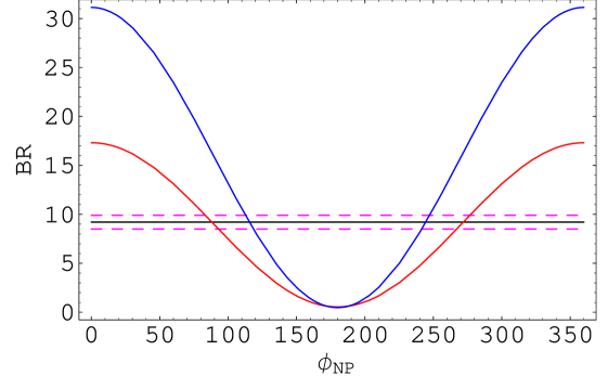
Now plotting the branching ratio (9) versus Ο•N​Psubscriptitalic-ϕ𝑁𝑃\phi_{NP} (the red line in Figure-1), we see that the observed data can be easily accommodated in
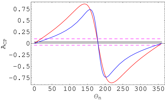
 VLDQ model. The direct CP asymmetry π’œCPsubscriptπ’œCP{\cal A}_{\rm CP} (Eq. (13) vs. ΞΈnsubscriptπœƒπ‘›\theta_{n} is plotted in Figure-2, for Ξ΄c=29∘subscript𝛿𝑐superscript29\delta_{c}=29^{\circ} and Ξ΄n=βˆ’5∘subscript𝛿𝑛superscript5\delta_{n}=-5^{\circ}, and it is also (the red line in Figure-2) in compatible with the present experimental data. Furthermore, it should be noted from the Figure-2 that VLDQ model can accommodate the CP violating asymmetry upto 85%percent8585\%.

Refer to caption

Figure 1: Branching ratio of $B^{-}\to\phi K^{-}$ process (in units of $10^{-6}$) versus the phase $\phi_{NP}$ (in degree). The red and blue curve represent the results of VLDQ and RPV model respectively. The horizontal solid line is the central experimental value whereas the dashed horizontal lines denote the error limits.

Refer to caption

Figure 2: The direct CP asymmetry (${\cal A}_{\rm CP}$) in the $B^{\pm}\to\phi K^{\pm}$ process versus the new weak phase $\theta_{n}$ (in degree). The red and blue curve represent the results of VLDQ and RPV model. The horizontal solid line is the central experimental value whereas the dashed horizontal lines denote the error limits.

5 Contribution from R-Parity violating supersymmetric model

We now analyze the decay mode in the minimal supersymmetric model with R-parity violation. In the supersymmetric models there may be interactions which violate the baryon number $B$ and the lepton number $L$ generically. The simultaneous presence of both $L$ and $B$ number violating operators induce rapid proton decay, which may contradict strict experimental bound. In order to keep the proton lifetime within experimental limit, one needs to impose additional symmetry beyond the SM gauge symmetry to force the unwanted baryon and lepton number violating interactions to vanish. In most cases this has been done by imposing a discrete symmetry called R-parity defined as, $R_{p}=(-1)^{(3B+L+2S)}$, where $S$ is the intrinsic spin of the particles. Thus the $R$-parity can be used to distinguish the particle ($R_{p}$=+1) from its superpartner ($R_{p}=-1$). This symmetry not only forbids rapid proton decay, it also renders stable the lightest supersymmetric particle (LSP). However, this symmetry is ad hoc in nature. There is no theoretical arguments in support of this discrete symmetry. Hence it is interesting to see the phenomenological consequences of the breaking of R-parity in such a way that either $B$ and $L$ number is violated, both are not simultaneously violated, thus avoiding rapid proton decay. Extensive studies has been done to look for the direct as well as indirect evidence of R-parity violation from different processes and to put constraints on various R-parity violating couplings. The most general $R$-parity and Lepton number violating super-potential is given as

$$W_{\not\!{L}}=\frac{1}{2}\lambda_{ijk}L_{i}L_{j}E_{k}^{c}+\lambda_{ijk}^{\prime}L_{i}Q_{j}D_{k}^{c}\;,$$ (41)

where, $i,j,k$ are generation indices, $L_{i}$ and $Q_{j}$ are $SU(2)$ doublet lepton and quark superfields and $E_{k}^{c}$, $D_{k}^{c}$ are lepton and down type quark singlet superfields. Further, $\lambda_{ijk}$ is antisymmetric under the interchange of the first two generation indices. Thus the relevant four fermion interaction induced by the R-parity and lepton number violating model is [23]

$\displaystyle{\cal H}_{\not\!{R}}$ $\displaystyle=$ $\displaystyle\frac{1}{8m^{2}_{\tilde{\nu}}}\biggr{[}(\lambda_{i23}^{\prime*}\lambda_{i22}^{\prime})(\bar{s}_{\alpha}\gamma^{\mu}(1-\gamma_{5})s_{\beta})~{}(\bar{s}_{\beta}\gamma_{\mu}(1+\gamma_{5})b_{\alpha})$ (42)
$\displaystyle\hskip 5.69046pt+(\lambda_{i32}^{\prime}\lambda_{i22}^{\prime*})(\bar{s}_{\alpha}\gamma^{\mu}(1+\gamma_{5})s_{\beta})~{}(\bar{s}_{\beta}\gamma_{\mu}(1-\gamma_{5})b_{\alpha})\biggr{]}\;.$

It should be noted that, the factorized matrix elements of both the operators in Eq. (42) are same because of

$\displaystyle\langle K^{-}|\bar{s}\gamma^{\mu}(1-\gamma_{5})b|B^{-}\rangle=\langle K^{-}|\bar{s}\gamma^{\mu}(1+\gamma_{5})b|B^{-}\rangle=\langle K^{-}|\bar{s}\gamma^{\mu}b|B^{-}\rangle\;,$
βŸ¨Ο•|s¯​γμ​(1βˆ’Ξ³5)​s|0⟩=βŸ¨Ο•|s¯​γμ​(1+Ξ³5)​s|0⟩=βŸ¨Ο•|s¯​γμ​s|0⟩.quantum-operator-productitalic-ϕ¯𝑠superscriptπ›Ύπœ‡1subscript𝛾5𝑠0quantum-operator-productitalic-ϕ¯𝑠superscriptπ›Ύπœ‡1subscript𝛾5𝑠0quantum-operator-productitalic-ϕ¯𝑠superscriptπ›Ύπœ‡π‘ 0\displaystyle\langle\phi|\bar{s}\gamma^{\mu}(1-\gamma_{5})s|0\rangle=\langle\phi|\bar{s}\gamma^{\mu}(1+\gamma_{5})s|0\rangle=\langle\phi|\bar{s}\gamma^{\mu}s|0\rangle\;. (43)

So, including the nonfactorizable effects, we obtain the R-parity violating contribution to the decay amplitude as

$\displaystyle A^{\not\!R}(B^{-}\to\phi K^{-})=\frac{1}{8m^{2}_{\tilde{\nu}}}\Big{(}\lambda_{i32}^{\prime}\lambda_{i22}^{\prime*}+\lambda_{i23}^{\prime*}\lambda_{i22}^{\prime}\Big{)}X\biggr{[}\frac{1}{N}+\frac{\alpha_{s}}{4\pi}\frac{C_{F}}{N}(-F_{\phi}-12)\biggr{]}\;,$ (44)

where the summation over $i=1,2,3$ is implied. Now considering the values of R-parity couplings from [5] as

$$-\frac{1}{24m^{2}_{\tilde{\nu}}}\Big{(}\lambda_{i32}^{\prime}\lambda_{i22}^{\prime*}+\lambda_{i23}^{\prime*}\lambda_{i22}^{\prime}\Big{)}=\frac{R}{12M^{2}}e^{i\theta_{n}}\;,$$ (45)

where $\theta_{n}$ is the new weak phase of R-parity violating couplings and $R\sim 1.5\times 10^{-3}$ for the mass scale $M\sim m_{\tilde{\nu}}=100$ GeV.

Thus we obtain the R-parity violating amplitude as

$$A^{RPV}(B\to\phi K^{-})=-(\epsilon\cdot p_{B})e^{i\theta_{n}}\left(2.462+i~{}0.512\right)\times 10^{-9}\;,$$ (46)

with the strong phase as $\sim 12^{\circ}$. Thus, the new physics contribution $r_{NP}$ is found to be

$$r_{NP}=1.28\;.$$ (47)

Plotting the branching ratio (9) vs. $\phi_{NP}$ we can see that the observed branching ratio can be easily accommodated in the RPV model (blue curve in Fig-1). Similarly the observed direct CP asymmetry can also be explained by RPV model, (blue curve in Figure-2). As can be seen from Fig-2, the RPV model can accommodate CP asymmetry upto 70$\%$.

6 Conclusion

The measured branching ratio and direct CP asymmetry parameter in the $B^{\pm}\to\phi K^{\pm}$ mode are not in agreement with the SM expectations. The direct CP asymmetry in this mode in the SM is expected to be very small (at $1\%$ level) but the measured value is higher than this. But this should be treated with caution since the error bars are still very large in comparison to the central value and definitive conclusion cannot be obtained. On the other hand there is a very wild speculation and/or a general belief that exist in the literature is that there might be some kind of new physics effect present, in the decay amplitude of the pure penguin process $B^{0}\to\phi K_{S}$, to account for the $2.7\sigma$ deviation of the measured $(\sin 2\beta)_{\phi K_{S}}$ from $(\sin 2\beta)_{\psi K_{S}}$. So it is quite obvious that presence of NP may not be ruled out on its charged counterpart process $B^{\pm}\to\phi K^{\pm}$ having the same underlying quark dynamics.

In fact there are various ways to test the presence of new physics that exist in the literature. One of them is to find nonzero direct CP asymmetry in modes which are dominated by a single decay amplitude in the SM and hence expected to give zero direct CP asymmetry. The mode $B^{\pm}\to\phi K^{\pm}$ falls into that class, where the ${\cal A}_{\rm CP}$ is expected to be negligibly small. But the present data do not seem to respect the same and may reveal hidden NP effects in future. In order to look for NP, we first carefully reanalyzed this mode ($B^{\pm}\to\phi K^{\pm}$) in the default QCD factorization approach. We also took into account of the small annihilation contribution in our calculation and found that the branching ratio and ${\cal A}_{\rm CP}$ are deviated from the present experimetal data. However, our results are in close agreement with the latest theoretical calculation [18].

We took this opportunity to incorporate the possible new physics scenarios to explain the same. In order to obtain significant direct CP asymmetry both the interfering amplitudes (i.e., the SM and NP amplitudes) should be of the same order and the relative phase differences between them should be nonvanishing. We then introduce two beyond the standard model scenarios in turn to explain the observed branching ratio and ${\cal A}_{\rm CP}$. These are the VLDQ model and the RPV supersymmetric model. These two models are shown in the literature that they can successfully explain the possible discrepancy of $B^{0}\to\phi K_{S}$ result with that of the SM expectation. We find that $r_{NP}$, which is the ratio between the NP and SM amplitudes, to be 0.7 and 1.28 for VLDQ and RPV model respectively. As can be seen now from the Figures-1 and 2, that these two models can also accommodate the possible deviation of branching ratio and CP asymmetry parameter from the SM values for the decay under consideration. Eventually, it turns out that direct CP asymmetry upto $\sim 85\%~{}(70\%)$ can be accommodated in the VLDQ (RPV) model, if nature is so obliged to give such a large value. In fact more precise data in future will lead us to definitive conclusions and/or narrow down some NP scenarios.

To conclude, the branching ratio and direct CP asymmetry parameter (${\cal A}_{\rm CP}$) as obtained in Belle and BABAR indicate deviation from that of the SM expectation in the $B^{\pm}\to\phi K^{\pm}$ decay. If the trend remains the same, as it is now, then it may lead to the establishment of the presence of new physics in penguin dominated ($b\to s\bar{s}s$) $B$ decays. At present it is too early to say anything in favor of or rule out the possibility of the existence of new physics in this sector. At the same time keeping in mind all these we should keep every option open, explore various possibilities and hope that $B$ factory data will reveal new physics in the near future.

7 Acknowledgments

AKG was supported by the Lady Davis Fellowship and the work of RM was supported in part by Department of Science and Technology, Government of India through Grant No. SR/FTP/PS-50/2001.

References

  • [1] BABAR Collaboration, B.Β Aubert et al. Phys. Rev. Lett. 89, 201802 (2002); Belle Collaboration, K. Abe et al., hep-ex/0207098.
  • [2] T. Browder, Talk presented at the Lepton-Photon, 2003, Int. J. Mod. Phys. A 19, 965 (2004).
  • [3] Y.Β Grossman and M.Β P.Β Worah, Phys.Β Lett.Β B 395, 241 (1997); D. London and A. Soni, Phys. Lett. B 407, 61 (1997); Y. Grossman, G. Isidori and M. Worah, Phys. Rev. D 58, 057504 (1997).
  • [4] G. Barenboim, J. Bernabeu and M. Raidal, Phys. Rev. Lett. 80, 4625 (1998); M. Raidal, Phys. Rev. Lett. 89, 231803 (2002); M. Ciuchini and L. Silverstini, Phys. Rev. Lett. 89, 231802 (2002); E. Lunghi and D. Wyler, Phys. Lett. B 521, 320 (2001); S. Khalil and E. Kou, Phys. Rev. D 67, 055009 (2003); G. L. Kane, P. Ko, H. Yang, C. Kolda, J.-H. Park and L. T. Yang, Phys. Rev. Lett. 90, 141803 (2003); K. Agashe and C. D. Carone, Phys. Rev. D 68, 035017 (2003); C.-W. Chiang and J. L. Rosner, Phys. Rev. D 68, 014007 (2003); J.-F. Cheng, C.-S. Huang and X.-H. Wu, Phys. Lett. B 585, 287 (2004); D. Chakraverty, E. Gabrielli, K. Huitu and S. Khalil, Phys. Rev. D 68, 095004 (2003); B. Dutta, C. S. Kim and S. Oh, Phys. Rev. Lett. 90, 011801 (2003); R. Arnowitt, B. Dutta and B. Hu, Phys. Rev. D 68, 075008 (2003); C.-S. Huang and S.-H. Zhu, Phys. Rev. D 68, 114020 (2003); V. Barger, C.-W. Chiang, P. Langacker and H-S Lee, Phys. Lett. B 580, 186 (2004) .
  • [5] A. Datta, Phys. Rev. D 66, 071702(R) (2002).
  • [6] G. Hiller, Phys. Rev. D 66, 071502(R) (2002).
  • [7] A. K. Giri and R. Mohanta, Phys. Rev. D 68, 014020 (2003).
  • [8] Belle Collaboration. K.- F. Chen et al, Phys. Rev. Lett. 91, 201801 (2003).
  • [9] BABAR Collaboration, B Aubert et al., Phys. Rev. D 69, 011102 (2004).
  • [10] CLEO Collboration, R. A. Briere et al., Phys. Rev. Lett. 86, 3718 (2001).
  • [11] M. Beneke, G. Buchalla, M. Neubert and C. T. Sachrajda, Phys. Rev. Lett. 83, 1914 (1999); Nucl. Phys. B 591, 313 (2000).
  • [12] M. Beneke, G. Buchalla, M. Neubert and C. T. Sachrajda, Nucl. Phys. B 606, 245 (2001).
  • [13] X. G. He, J. P Ma and C. Y. Wu, Phys. Rev. D 63, 094004 (2001).
  • [14] H. Y. Cheng and K. C. Yang, Phys. Rev. D 64, 074004 (2001).
  • [15] D. Du, H. Gong, J. Sun. D. Yang and G. Zhu, Phys. Rev. D 65, 094025 (2002); Erratum, Phys. Rev. D 66, 079904 (2002).
  • [16] G.Β Buchalla, A.J.Β Buras, M.Β Lautenbacher, Rev.Β Mod.Β Phys.Β 68 (1996) 1125.
  • [17] M. Z. Yang and Y. D. Yang, Phys. Rev. D 62, 114019 (2000).
  • [18] M. Beneke and M. Neubert, hep-ph/0308039 (to appear in Nucl. Phys. B).
  • [19] M. Neubert, Talk presented at 3rd International School on CP violation and Heavy Quark Physics, Prerow, Germany, (22-26 Sept. 2003).
  • [20] M.Β Wirbel, M.Β Bauer, B.Β Stech, Z. Phys. C 29, 637 (1985); ibid 34, 103 (1987).
  • [21] Particle Data Group, K. Hagiwara et al., Phys. Rev D. 66, 010001 (2002).
  • [22] Y. Grossman, Y. Nir and R. Rattazzi, in Heavy Flavours II, edited by A. J. Buras and M. Lindner, (World Scientific, Singapore), 1998, p. 755.
  • [23] D. Guetta, Phys. Rev. D 58, 116008 (1998); B. Dutta, C. S. Kim and S. Oh, Phys. Rev. Lett. 90, 011801 (2003).