Abstract

The purpose of the present paper is to study the neutrino properties as they may appear in the low energy neutrinos emitted in triton decay:

$${}^{3}_{1}H\rightarrow^{3}_{2}He+e^{-}+\tilde{\nu}_{e}$$

with maximum neutrino energy of $18.6~{}KeV$. The technical challenges to this end can be summarized as building a very large TPC capable of detecting low energy recoils, down to a few 100 eV, within the required low background constraints. More specifically We propose the development of a spherical gaseous TPC of about 10-m in radius and a 200 Mcurie triton source in the center of curvature. One can list a number of exciting studies, concerning fundamental physics issues, that could be made using a large volume TPC and low energy antineutrinos: 1) The oscillation length involving the small angle $\delta=\sin{\theta_{13}}$, directly measured in our $\nu_{e}$ disappearance experiment, is fully contained inside the detector. Measuring the counting rate of neutrino-electron elastic scattering as function of the distance of the source will give a precise and unambiguous measurement of the oscillation parameters free of systematic errors. In fact first estimations show that even with a year’s data taking a sensitivity of a few percent for the measurement of the above angle will be achieved. 2) The low energy detection threshold offers a unique sensitivity for the neutrino magnetic moment which is about two orders of magnitude beyond the current experimental limit of $10^{-10}\mu_{B}$. 3) Scattering at such low neutrino energies has never been studied and any departure from the expected behavior may be an indication of new physics beyond the standard model. We present a summary of various theoretical studies and possible measurements, including a precise measurement of the Weinberg angle at very low momentum transfer.

1 Introduction.

Neutrinos are the only particles in nature, which are characterized by weak interactions only. They are thus expected to provide the laboratory for understanding the fundamental laws of nature. Furthermore they are electrically neutral particles characterized by a very small mass. Thus it is an open question whether they are truly neutral, in which case the particle coincides with its own antiparticle , i.e. they are Majorana particles, or they are characterized by some charge, in which case they are of the Dirac type, i.e the particle is different from its antiparticle [1]. It is also expected that the neutrinos produced in weak interactions are not eigenstates of the world Hamiltonian, they are not stationary states, in which case one expects them to exhibit oscillations [1, 2] . As a matter of fact such neutrino oscillations seem to have observed in atmospheric neutrino [3], interpreted as $\nu_{\mu}\rightarrow\nu_{\tau}$ oscillations, as well as $\nu_{e}$ disappearance in solar neutrinos [4]. These results have been recently confirmed by the KamLAND experiment [5], which exhibits evidence for reactor antineutrino disappearance. This has been followed by an avalanche of interesting analyses [6]-[10]. The purpose of the present paper is to discuss a new experiment to study the above neutrino properties as they may appear in the low energy neutrinos emitted in triton decay:

$${}^{3}_{1}H\rightarrow^{3}_{2}He+e^{-}+\tilde{\nu}_{e}$$

with maximum neutrino energy of $18.6~{}KeV$. This process has previously been suggested [11] as a means of studying heavy neutrinos like the now extinct $17KeV$ neutrino. The detection will be accomplished employing gaseous Micromegas,large TPC (Time Projection Counters) detectors with good energy resolution and low background [12]. In addition in this new experiment we hope to observe or set much more stringent constraints on the neutrino magnetic moments. This very interesting question has been around for a number of years and it has been revived recently [13]-[16]. The existence of the neutrino magnetic moment can be demonstrated either in neutrino oscillations in the presence of strong magnetic fields or in electron neutrino scattering. The latter is expected to dominate over the weak interaction in the triton experiment since the energy of the outgoing electron is very small. Furthermore the possibility of directional experiments will provide additional interesting signatures. Even experiments involving polarized electron targets are beginning to be contemplated [17]. There are a number of exciting studies, of fundamental physics issues, that could be made using a large volume TPC and low energy antineutrinos:

• The oscillation length is comparable to the length of the detector. Measuring the counting rate of neutrino elastic scattering as function of the distance of the source will give a precise and unambiguous measurement of the oscillation parameters free of systematic errors. First estimations show that a sensitivity of a few percent for the measurement of $\sin^{2}{\theta_{13}}$.

• The low energy detection threshold offers a unique sensitivity for the neutrino magnetic moment, which is about two orders of magnitude beyond the current experimental limit of $10^{-10}\mu_{B}$. In our estimates below we will use the optimistic value of $10^{-12}\mu_{B}$.

• Scattering at such low neutrino energies has never been studied before. In addition one may exploit the extra signature provided by the photon in radiative electron neutrino scattering. As a result any departure from the expected behavior may be an indication of physics beyond the standard model.

In the following we will present a summary of various theoretical studies and possible novel measurements

2 Neutrino masses as extracted from various experiments

At this point it instructive to elaborate a little bit on the neutrino mass combinations entering various experiments.

• Cosmological Constraints. We get [18, 19]:

  $$\Omega_{\nu}~{}h^{2}\leq 0.0076(95\%~{}CL)$$

  $$\frac{\Sigma_{i}~{}m_{i}}{93.5~{}eV}=\Omega_{\nu}~{}h^{2}\Rightarrow$$

  $$\Sigma_{i}~{}m_{i}\leq 0.71~{}eV/c^{2}~{}~{}(95\%~{}CL)$$

  (Majorana neutrinos).
  The limit becomes $1.05~{}eV$ without the Ly-$\alpha$ forest data For Dirac neutrinos the value of the upper limit is half the above.

• Neutrino oscillations.
  These in principle, determine the mixing matrix and two independent mass-squared differences, e.g.

  $$\Delta m^{2}_{21}=m^{2}_{2}-m^{2}_{1}~{}~{},~{}~{}\Delta m^{2}_{31}=m^{2}_{3}-m^{2}_{1}$$

  They cannot determine:

  1. the scale of the masses, e.g. the lowest eigenvalue $m_{1}$ and

  2. the two relative Majorana phases.

• The end point triton decay.

  This can determine one of the masses, e.g. $m_{1}$ by measuring:

  $$(m_{\nu})_{1\beta}\equiv m_{\nu}=|\sum_{j=1}^{3}U^{*}_{ej}U_{ej}m^{2}_{j}|^{1/2}\,,~{}U=U^{11}$$ (1)

  Once $m_{1}$ is known one can find
  

  $$m_{2}=[\delta m^{2}_{21}+m^{2}_{1}]^{1/2}~{}~{},~{}~{}m_{3}=[\delta m^{2}_{31}+m^{2}_{1}]^{1/2}$$

  provided, of course that the mixing matrix is known.
  Since the Majorana phases do not appear, this experiment cannot differentiate between Dirac and Majorana neutrinos. This can only be done via lepton violating processes, like:

• $0\nu\beta\beta$ decay.

  This provides an additional independent linear combinations of the masses and the Majorana phases.

  $$\langle m_{\nu}\rangle_{2\beta}\equiv\langle m_{\nu}\rangle=|\sum_{j=1}^{3}U_{ej}U_{ej}e^{i\lambda_{j}}m_{j}|$$ (2)

• and muon to positron conversion.

  This also provides an additional relation

  $$\langle m_{\nu}\rangle_{\mu e+}=|\sum_{j=1}^{3}U^{*}_{\mu j}U^{*}_{ej}e^{-i\lambda_{j}}m_{j}|\,.$$ (3)

Thus the two independent relative CP phases can in principle be measurable. So these three types of experiments together can specify all parameters not settled by the neutrino oscillation experiments.

Anyway from the neutrino oscillation data alone we cannot infer the mass scale. Thus the following scenarios emerge

1. the lightest neutrino is $m_{1}$ and its mass is very small. This is the normal hierarchy scenario. Then:

   $$\Delta m^{2}_{21}=m^{2}_{2}~{}~{},~{}~{}\Delta m^{2}_{31}=m^{2}_{3}$$

2. The inverted hierarchy scenario. In this case the mass $m_{3}$ is very small. Then:

   $$\Delta m^{2}_{21}=m^{2}_{2}-m^{2}_{1}~{}~{},~{}~{}\Delta m^{2}_{31}=m^{2}_{1}$$

3. The degenerate scenario. In such a situation all masses are about equal and much larger than the differences appearing in neutrino oscillations. In this case we can obtain limits on the mass scale as follows:

   • From triton decay. Then [20]

     $$m_{1}\approx(m_{\nu})_{1\beta}\leq 2.2eV$$

     This limit is expected to substantially improve in the future [21].

   • From $0\nu~{}\beta\beta$ decay. The analysis now depends on the mixing matrix and the CP phases of the Majorana neutrino eigenstates [1] (see discussion below). The best limit coming from $0\nu~{}\beta\beta$ decay is:

     $$m_{1}\approx\langle m_{\nu}\rangle_{2\beta}\leq 0.5~{}eV,m_{1}\approx\frac{\langle m_{\nu}\rangle_{2\beta}}{\cos{2\theta_{solar}}}\approx 2\langle m_{\nu}\rangle_{2\beta}\leq 1.0~{}eV,$$

     for relative CP phase of the two strongly admixed states is $0$ and $\pi$ respectively.

     These limits are going to greatly improve in the next generation of experiments, see e.g. the review by Vergados [1] and the experimental references therein.

3 Elastic electron neutrino scattering.

The elastic neutrino electron scattering, which has played an important role in physics [22], is very crucial in our investigation, since it will be employed for the detection of neutrinos. So we will briefly discuss it before we embark on the discussion of the apparatus.

Following the pioneering work of ’t Hooft [23] as well as the subsequent work of Vogel and Engel [13] one can write the relevant differential cross section as follows:

$$\frac{d\sigma}{dT}=\left(\frac{d\sigma}{dT}\right)_{weak}+\left(\frac{d\sigma}{dT}\right)_{EM}$$ (4)

We ignored the contribution due to the neutrino charged radius. We will not consider separately the scattering of electrons bound in the atoms, since such effects have recently been found to be small [24].

The cross section due to weak interaction alone takes the form [13]:

$$\left(\frac{d\sigma}{dT}\right)_{weak} = \frac{G^{2}_{F}m_{e}}{2\pi}[(g_{V}+g_{A})^{2}+(g_{V}-g_{A})^{2}(1-\frac{T}{E_{\nu}})^{2}$$

$$+ (g_{A}^{2}-g_{V}^{2})\frac{m_{e}T}{E^{2}_{\nu}}]$$

where

$$g_{V}=2\sin^{2}\theta_{W}+1/2~{}~{}for~{}~{}\nu_{e}~{}~{}~{}~{},~{}~{}~{}~{}g_{V}=2\sin^{2}\theta_{W}-1/2~{}~{}for~{}~{}\nu_{\mu},\nu_{\tau}$$

$$g_{A}=1/2~{}~{}for~{}~{}\nu_{e}~{}~{}~{}~{},~{}~{}~{}~{}g_{A}=-1/2~{}~{}for~{}~{}\nu_{\mu},\nu_{\tau}$$

For antineutrinos $g_{A}\rightarrow-g_{A}$. To set the scale we see that

$$\frac{G^{2}_{F}m_{e}}{2\pi}=0.445\times 10^{-48}~{}\frac{m^{2}}{MeV}$$ (6)

In the above expressions for the $\nu_{\mu},\nu_{\tau}$ only the neutral current has been included, while for $\nu_{e}$ both the neutral and the charged current contribute.

The second piece of the cross-section becomes:

$$\left(\frac{d\sigma}{dT}\right)_{EM}=\pi(\frac{\alpha}{m_{e}})^{2}(\frac{\mu_{l}}{\mu_{B}})^{2}\frac{1}{T}\left(1-\frac{T}{E_{\nu}}\right)$$ (7)

where in the mass basis $\mu_{l}^{2}$ takes the form

$$\mu^{2}_{l}=|c^{2}\mu_{11}+s^{2}\mu_{22}|^{2}$$

$$\mu^{2}_{l}=\mu^{2}_{21}~{}+~{}|c~{}\mu_{31}~{}+~{}s~{}exp(i\alpha_{CP})~{}\mu_{32}|^{2}$$

for Dirac and Majorana neutrinos respectively. For the definition of $c$ and $s$ see sec. 5 below. In the case of Dirac neutrinos the off diagonal elements of the magnetic moment were meglected. The angle $\alpha_{CP}$ is the relative CP phase of of the dominant neutrino Majorana mass eigenstates present in the electronic neutrino. The contribution of the magnetic moment can also be written as:

$$\left(\frac{d\sigma}{dT}\right)_{EM}=\sigma_{0}\left(\frac{\mu_{l}}{10^{-12}\mu_{B}}\right)^{2}\frac{1}{T}\left(1-\frac{T}{E_{\nu}}\right)$$ (8)

The quantity $\sigma_{0}$ sets the scale for the cross section and is quite small, $\sigma_{0}=2.5\times 10^{-25}b$.

The electron energy depends on the neutrino energy and the scattering angle and is given by:

$$T\approx\frac{2(E_{\nu}\cos{\theta})^{2}}{m_{e}}$$

For $E_{\nu}=18.6~{}KeV$ one finds that the maximum electron kinetic energy approximately is [12]:

$$T_{max}=1.27~{}KeV$$

Integrating the differential cross section between $0.1$ and $1.27~{}KeV$ we find that the total cross section is:

$$\sigma=2.5~{}\sigma_{0}$$

It is tempting for comparison to express the above EM differential cross section in terms of the weak interaction, near the threshold of $0.1KeV$, as follows:

$$\left(\frac{d\sigma}{dT}\right)_{EM}=\xi^{2}_{1}\left(\frac{d\sigma}{dT}\right)_{Weak}\left(\frac{\mu_{l}}{10^{-12}\mu_{B}}\right)^{2}\frac{0.1KeV}{T}\left(1-\frac{T}{E_{\nu}}\right)$$ (9)

The parameter $\xi_{1}$ essentially gives the ratio of the interaction due to the magnetic moment divided by that of the weak interaction. Evaluated at the energy of $0.1KeV$ it becomes:

$$\xi_{1}\approx 0.50$$

Its value, of course, will be larger if the magnetic moment is larger than $10^{-12}\mu_{B}$. Anyway the magnetic moment at these low energies can make a detectable contribution provided that it is not much smaller than $10^{-12}\mu_{B}$. In many cases one would like to know the difference between the cross section of the electronic neutrino and that of one of the other flavors, i.e.

$$\chi(E_{\nu},T)=\frac{(d\sigma(\nu_{e},e^{-}))/dT-d(\sigma(\nu_{\alpha},e^{-}))/dT}{d(\sigma(\nu_{e},e^{-}))/dT}$$ (10)

with $\nu_{\alpha}$ is either $\nu_{\mu}$ or $\nu_{\tau}$). Then from the above expression for the differential cross-section one finds:

$$\chi=2[\frac{2-(m_{e}T/E^{2}_{\nu})}{ff1(\theta_{W})+2sin^{2}\theta_{W}(1-T/E_{\nu})^{2}-ff2(\theta_{W})(m_{e}T/E^{2}_{\nu}}$$ (11)

with

$$ff1(\theta_{W})=(1+2\sin^{2}\theta_{W})^{2}/(2sin^{2}\theta_{W})~{}~{},~{}~{}ff2(\theta_{W})=(1+2\sin^{2}\theta_{W})$$

For antineutrinos the above equation is slightly modified to yield

$$\chi=2[\frac{2-(m_{e}T/E^{2}_{\nu})}{2sin^{2}\theta_{W}+ff1(\theta_{w})(1-T/E_{\nu})^{2}-ff2(\theta_{W})(m_{e}T/E^{2}_{\nu}}$$ (12)

Specializing Eq. 3 in the case of the antineutrino-electron scattering we get:

$$\left(\frac{d\sigma}{dT}\right)_{weak} = \frac{G^{2}_{F}m_{e}}{2\pi}$$

$$[(2sin^{2}\theta_{W})^{2}+(1+2\sin^{2}\theta_{W})^{2}(1-T/E_{\nu})^{2}$$

$$- 2sin^{2}\theta_{W}(1+2\sin^{2}\theta_{W})(m_{e}T/E^{2}_{\nu})]$$

This last equation can be used to measure $\sin^{2}\theta_{W}$ at very low momentum transfers, almost 30 years after the first historic measurement by Reiness, Gur and Sobel [22]. In the present experiment we will measure the differential cross section as a function of $T$, which is a essentially a straight line. With sufficient statistics we expect to construct the straight line sufficiently accurately, so that we can extract $\sin^{2}\theta_{W}$ both from the slope and the intercept achieving high precision. We should mention that the present method does not suffer from the well known supression of the weak charge associated with other low energy processes [25] including the atomic physics experiments [26, 27]. This is due to the fact that the dependence on the Weinberg angle in these experiments comes from the neutral current vector coupling of the electron and/or the proton, involving the combination $1-4\sin^{2}\theta_{W}\approx 0.1$. Thus in our approach it may not be necessary to go through an elaborate scheme of radiative corrections (see the recent work by Erler et al [28] and references therein).

4 Experimental considerations

In this section we will focus on the experimental considerations

One of the attractive features of the gaseous TPC is its ability to precisely reconstruct particle trajectories without precedent in the redundancy of experimental points, i.e. a bubble chamber quality with higher accuracy and real time recording of the events. Many proposals are actually under investigation to exploit the TPC advantages for various astroparticle projects and especially solar or reactor neutrino detection and dark matter search [29]-[32]. A common goal is to fully reconstruct the direction of the recoil particle trajectory, which together with energy determination provide a valuable piece of information. The virtue of using the TPC concept in such investigations has been now widely recognized and a special International Workshop has been recently organized in Paris [33]. The study of low energy elastic neutrino-electron scattering using a strong tritium source was envisaged in by Bouchez and Giomataris [34] employing a large volume gaseous cylindrical TPC. We will present here an alternate detector concept with different experimental strategy based on a spherical TPC design. A sketch of the principal features of the proposed TPC is shown in Fig. 1.

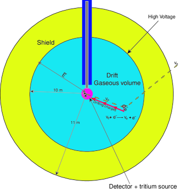
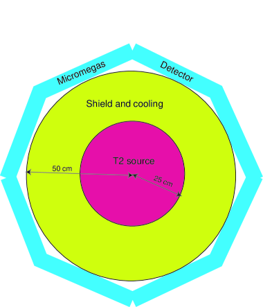
Figure 1: The principal features of the proposed TPC (a) and a schematic view of the inner part of the vessel with the detector and the tritium source (right).

For a more detailed description of the apparatus, including the neutrino source, the gas vessel and detailed study of the detector [38, 39], [40, 41] including a discussion of MICROMEGAS (MICROMEsh GAseous Structure) [42, 43, 44] the reader is referred to our previous work [45].

Our approach is radically different from all other neutrino oscillation experiments in that it measures the neutrino interactions, as a function of the distance source-interaction point, with an oscillation length that is fully contained in the detector; it is equivalent to many experiments made in the conventional way where the neutrino flux is measured in a single space point. Furthermore, since the oscillation length is comparable to the detector depth, we expect an exceptional signature: a counting rate oscillating from the triton source location to the depth of the gas volume, i.e. at first a decrease, then a minimum and finally an increase. In other words we will have a full observation of the oscillation process as it has already been done in accelerator experiments with neutral strange particles ($K^{0}$).

To summarize:

• The aim of the proposed detector will be the detection of very low energy neutrinos emitted by a strong tritium source through their elastic scattering on electrons of the target.

• The $(\nu,e)$ elastic differential cross section is the sum of the charged and neutral current contributions (see sec. 3) and is a function of the energy. It is, however, it is quite small, see Eq. (6).

• Integrating this cross section up to energies of $15~{}KeV$ we get a very small value, $\sigma=0.4\times 10^{-47}cm^{2}$. This means that, to get a significant signal in the detector, for 200 Mcurie tritium source (see next section) we will need about 20 kilotons of gaseous material.

• The elastic $(\nu,e)$ cross section, being dominated by the charged current, especially for low energy electrons (see Fig. 19 below), will be different from that of the other flavors, which is due to the neutral current alone. This will allow us to observe neutrino oscillation enabling a modulation on the counting rate along the oscillation length. The effect depends on the electron energy T as is shown in sec. 5

We assume a spherical type detector, described in the previous section, filed with Xenon gas at NTP and a tritium source of 20 kg, providing a very-high intensity neutrino emission of $6\times 10^{18}/s$. The Monte Carlo program is simulating all the relevant processes:

• Beta decay and neutrino energy random generation

• Oscillation process of $\nu_{e}$ due to the small mixing $\theta_{13}$ (see Eq. 14 below).

• Neutrino elastic scattering with electrons of the gas target

• Energy deposition, ionization processes and transport of charges to the Micromegas detector.

First Monte Carlo simulate are giving a resolution of better than 10 cm, which is good enough for our need. In Fig. 2 the energy distribution of the detected neutrinos, assuming a detection threshold of 200 eV, is exhibited. The energy is concentrated around 13 keV with a small tail to lower values.

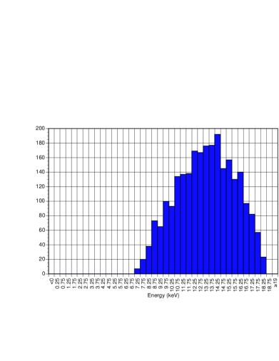
Figure 2: Neutrino energy distribution with an imposed energy cutoff of $200~{}eV$.

In Figs 5 and 6 below we show the number of detected elastic events as function of the distance L in bins of one meter for several hypothesis for the value of the mixing angle $\theta^{2}_{13}=0.170,0.085$ and $0.045$. We observe a decreasing of the signal up to about 6.5 m and then a rise. Backgrounds are not yet included in this simulation but the result looks quite promising; even in the case of the lowest mixing angle the oscillation is seen, despite statistical fluctuations. We should point out that in the context of this experiment complete elimination of the backgrounds is not necessary. It is worth noting that:

• A source-off measurement at the beginning of the experiment will yield the background level to be subtracted from the signal.

• Fitting the observed oscillation pattern will provide, for the first time, a stand alone measurement of the oscillation parameters, the mixing angle and the square mass square difference.

• Systematic effects due to backgrounds or to bad estimates of the neutrino flux, which is the main worry in most of the neutrino experiments, are highly reduced in this experiment.

5 A simple phenomenological neutrino mixing matrix- Simple expressions for neutrino oscillations

The available neutrino oscillation data (solar [4] and atmospheric [3])as well as the KamLAND [5] results can adequately be described by the following matrix:

$\left(\begin{array}[]{c}\nu_{e}\\ \nu_{\mu}\\ \nu_{\tau}\end{array}\right)=\left(\begin{array}[]{ccc}c&s&\delta\\ -\frac{s+c\delta}{\sqrt{2}}&\frac{c-s\delta}{\sqrt{2}}&\frac{1}{\sqrt{2}}\\ \frac{s-c\delta}{\sqrt{2}}&-\frac{c+s\delta}{\sqrt{2}}&\frac{1}{\sqrt{2}}\\ \end{array}\right)=\left(\begin{array}[]{c}\nu_{1}\\ \nu_{2}\\ \nu_{3}\end{array}\right)$

Up to order $\delta^{2}$ ($\delta^{2}=4\times 10^{-2}$). Sometimes we will use $\theta_{13}$ instead of $\delta$. Knowledge of this angle is very crucial for CP violation in the leptonic sector, since it may complex even if the neutrinos are Dirac particles. In the above expressions we have not absorbed the phases arising, if the neutrinos happen to be Majorana particles,$\nu_{k}\xi_{k}=C~{}{\overline{\nu}}_{k}^{T}$ where C denotes the charge conjugation, $\xi_{k}=e^{i\lambda_{k}}$, which guarantee that the eigenmasses are positive. The other entries are:

$$c=\cos\theta_{solar}~{},~{}s=\sin\theta_{solar}$$

determined from the solar neutrino data [4], [6]-[10]

$$\tan^{2}\theta_{solar}\approx 0.35-0.42$$

$$0.26\leq\tan^{2}\theta_{solar}\leq 0.85~{}~{}(3\sigma)$$

while the analysis of KamLAND results [6]-[10] yields:

$$\tan^{2}\theta_{solar}\approx 0.46-0.64$$

$$0.29\leq\tan^{2}\theta_{solar}\leq 0.86~{}~{}(3\sigma)$$

• Solar neutrino Oscillation (LMA solution) is given by:

  $$P(\nu_{e}\rightarrow\nu_{e})\approx 1-(\sin 2\theta_{solar})^{2}\sin^{2}(\pi\frac{L}{L_{21}})$$

  $$L_{21}=\frac{4\pi E_{\nu}}{\Delta m^{2}_{21}}$$

  The analysis of both the neutrino oscillation experiments as well as KamLAND [6]-[10] yield

  $$\Delta m^{2}_{21}=|m_{2}^{2}-m_{1}^{2}|=(5.0-7.5)\times 10^{-5}(eV)^{2}$$

• The Atmospheric Neutrino Oscillation takes the form:

  $$P(\nu_{\mu}\rightarrow\nu_{\tau})=\sin^{2}(\pi\frac{L}{L_{32}})$$

  $$L_{32}=\frac{4\pi E_{\nu}}{\Delta m^{2}_{32}}\rightarrow\Delta m^{2}_{32}=|m_{3}^{2}-m_{2}^{2}|=2.5\times 10^{-3}(eV)^{2}$$

• We conventionally write

  $$\Delta m^{2}_{32}=\Delta m_{atm}^{2}~{}~{},~{}~{}\Delta m^{2}_{21}=\Delta m_{sol}^{2}$$

• Corrections to disappearance experiments

  $$P(\nu_{e}\rightarrow\nu_{e})=1-\frac{(\sin 2\theta_{solar})^{2}\sin^{2}(\pi\frac{L}{L_{21}})+4\delta^{2}\sin^{2}(\pi\frac{L}{L_{32}})}{(1+\delta^{2})^{2}}$$ (14)

• The probability for $\nu_{e}\rightarrow\nu_{\mu}$ oscillation takes the form:

  $$P(\nu_{e}\rightarrow\nu_{\mu}) = \frac{\left[(\sin 2\theta_{solar})^{2}+\delta\sin{4\theta_{solar}}\right]\sin^{2}(\pi\frac{L}{L_{21}})}{(1+\delta^{2})^{2}}$$

  $$+ \frac{4\delta^{2}\sin^{2}(\pi\frac{L}{L_{32}})}{(1+\delta^{2})^{2}}$$

• While the oscillation probability $\nu_{e}\rightarrow\nu_{\tau}$ becomes:

  $$P(\nu_{e}\rightarrow\nu_{\tau}) = \frac{\left[(\sin 2\theta_{solar})^{2}-\delta\sin{4\theta_{solar}}\right]\sin^{2}(\pi\frac{L}{L_{21}})}{(1+\delta^{2})^{2}}$$

  $$+ \frac{4\delta^{2}\sin^{2}(\pi\frac{L}{L_{32}})}{(1+\delta^{2})^{2}}$$

From the above expression we see that the small amplitude $\delta$ term dominates in the case of triton neutrinos ($L\leq L_{32}~{},L_{21}=50L_{32}$). In a different notation $4\delta^{2}\approx sin^{2}{2\theta_{13}}$

In the proposed experiment the neutrinos will be detected via the recoiling electrons. If the neutrino-electron cross section were the same for all neutrino species one would not observe any oscillation at all. We know, however, that the electron neutrinos behave very differently due to the charged current contribution, which is not present in the other neutrino flavors. Thus the number of the observed electron events ($ELEV$) will vary as a function of $L/E_{\nu}$ as follows:

$$ELEV \propto\frac{d(\sigma(\nu_{e},e^{-}))}{dT}$$

$$\left[1-\chi(E_{\nu},T)\frac{(\sin 2\theta_{solar})^{2}\sin^{2}(\pi\frac{L}{L_{21}})+4\delta^{2}\sin^{2}(\pi\frac{L}{L_{32}})}{(1+\delta^{2})^{2}}\right]$$

where

$$\chi(E_{\nu},T)=\frac{(d\sigma(\nu_{e},e^{-}))/dT-d(\sigma(\nu_{\alpha},e^{-}))/dT}{d(\sigma(\nu_{e},e^{-}))/dT}$$

($\nu_{\alpha}$ is either $\nu_{\mu}$ or $\nu_{\tau}$). In other words $\chi$ represents the fraction of the $\nu_{e}$-electron cross-section, $\sigma(\nu_{e},e^{-})$, which is not due to the neutral current. Thus the apparent disappearance oscillation probability will be quenched by this fraction. As we will see below, see section 3, the parameter $\chi$, for $sin^{2}\theta_{W}=0.2319$, can be cast in the form:

$$\chi(E_{\nu},T)=\frac{2[2-(m_{e}T/E^{2}_{\nu})]}{4.6199+0.4638(1-T/E{\nu})^{2}-1.4638(m_{e}T/E^{2}_{\nu})}$$ (19)

For antineutrinos the previous expression becomes:

$$\chi(E_{\nu},T)=\frac{2[2-(m_{e}T/E^{2}_{\nu})]}{0.46384+4.6199(1-T/E{\nu})^{2}-1.4638(m_{e}T/E^{2}_{\nu})}$$ (20)

We thus see that the parameter $\chi$ depends not only on the neutrino energy, but on the electron energy as well, see Figs 3-4. Since in our experiment $T$ is very low there is no essential difference between the two expressions for $\chi$.

Figure 3: The parameter $\chi$ as a function of the electron kinetic energy T for $E_{\nu}=9.0~{}KeV$ on the left and $12.0~{}KeV$ on the right.

Figure 4: The parameter $\chi$ as a function of the electron kinetic energy T for $E_{\nu}=15.0~{}KeV$ on the left and $18.0~{}KeV$ on the right.

It interesting to see that, for a given neutrino energy, $\chi$, as a function of $T$, is almost a straight line. We notice that, for large values of $T$, the factor $\chi$ is suppressed, which is another way of saying that, in this regime, in the case of $(\nu_{e},e^{-})$ differential cross-section the charged current contribution is cancelled by that of the neutral current.

In order to simplify the analysis one may try to replace $\chi$ by an average value $\bar{\chi}(E_{\nu})$, e.g. defined by:

$$\bar{\chi}(E_{\nu})=\frac{1}{T_{max}(E_{\nu})}\int_{0}^{T_{max}(E_{\nu})}\chi(E_{\nu},T)~{}dT$$ (21)

Then surprisingly one finds $\bar{\chi}(E_{\nu})$ is independent of $E_{\nu}$ with a constant value of $0.42$. This is perhaps a rather high price one may have to pay for detecting the neutrino oscillations as proposed in this work. One may turn this into an advantage, however, since the disappearance dip in Eq. LABEL:eventeq, in addition to its dependence on the familiar parameters , it also depends on the electron energy.

Anyway in the experiment involving a triton target one will actually observe a sinusoidal oscillation as a function of the source-detector distance $L$ with an amplitude, which is proportional to the square of the small mixing angle $\delta$. The relevant oscillation length is given by:

$$L_{32}=2.476m\frac{E_{\nu}(MeV)}{\Delta m^{2}_{32}((eV)^{2})}$$

In the present experiment for an average neutrino energy $E_{\nu}\approx 13KeV$ and $\Delta m^{2}_{32}=2.5\times 10^{-3}(eV)^{2}$ we find

$$L_{32}\approx 13.5m$$

In other words the maximum will occur close to the source at about $L=7.5m$. Simulations of the above neutrino oscillation involving $\nu_{e}$ disappearance due to the large $\Delta m^{2}=2.5\times 10^{-3}$, i.e associated with the small mixing $\delta$, are shown in Figs 5- 6. One clearly sees that the expected oscillation, present even for $\sin{2\theta_{13}}^{2}$. as low as $0.045$, will occur well inside the detector.

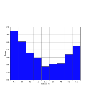
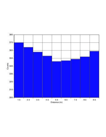
Figure 5: Simulation of $\nu_{e}$ disappearance due to the large $\Delta m^{2}=2.5\times 10^{-3}(eV)^{2}$ involving the small mixing angle $\sin{2\theta_{13}}^{2}$. The parameter $\chi(E_{\nu},T)$ was not included in making the plots. On the left we show results for $\sin{2\theta_{13}}^{2}=0.170$ , while on the right we show results for $\sin{2\theta_{13}}^{2}=0.085$. One expects to unambiguously see the full oscillation inside the detector with the maximum disappearance occurring around $6.5m$.

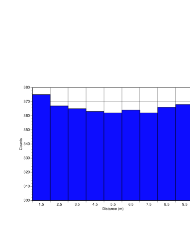
Figure 6: The same as in Fig. 5 for $\sin{2\theta_{13}}^{2}=0.045$.

Superimposed on this oscillation one will see an effect due to the smaller mass difference, which will increase quadratically with the distance $L$.

The above simple neutrino oscillation formulas get modified i) In the presence of a magnetic field if the neutrino has a magnetic moment and/or ii) If the heavier neutrinos have a finite life time. sectionRadiative neutrino-electron scattering The radiative neutrino decay for low energy neutrinos is perhaps unobservable. Radiative neutrino decay in the presence of matter, in our case electrons, is however observable.

$$\nu_{e}(p_{\nu})+e^{-}\longrightarrow\nu_{e}(p^{{}^{\prime}}_{\nu})+e^{-}(p_{e})+\gamma(k)$$

This occurs via the collaborative effect of electromagnetic and weak interactions as is shown in Fig. 7.

Figure 7: The Feynman diagrams contributing to radiative neutrino electron scattering via the charged current (left) and neutral current (right).

The evaluation of the cross section associated with these diagrams is rather complicated, but in the present case the electrons are extremely non relativistic. Thus in intermediate electron propagator we can retain the mass rather than the momenta by writing (see Fig. 7) $(p_{i}-k)^{\mu}\gamma_{\mu}+m_{e}\approx 2m_{e}$, $(p_{f}+k)^{\mu}\gamma_{\mu}+m_{e}\approx 2m_{e}$ (exact results without this approximation will appear elsewhere). Then after some tedious, but straight-forward, trace calculations one can perform the angular integrals over the three-body final states. Thus to leading order in the electron energy one gets:

$$k\frac{d\sigma(k,T_{e})}{dT_{e}~{}dk} = \sigma_{\gamma}\frac{m_{e}}{2\bar{E}^{2}_{\nu}}[(1-\frac{k}{E_{\nu}})g_{V}^{2}$$

$$+ \left(\frac{E^{2}_{\nu}}{m_{e}^{2}}(1-\frac{k}{E_{\nu}})-\frac{1}{8}(4g^{2}_{V}+g_{V}g_{A})\right)\frac{T_{e}~{}m_{e}}{E^{2}_{\nu}}]$$

where $\bar{E}_{\nu}=13.0~{}KeV$ is the average neutrino energy and

$$\sigma_{\gamma}=4\frac{8}{\pi^{2}}(G_{F}~{}\bar{E}_{\nu})^{2}~{}\alpha\approx 2.0\times 10^{-13}pb$$

sets the scale for this process. This momentum depends on the photon momentum k and the scattering angles. For a given $k$ is restricted as follows:

$$0\leq T_{e}\leq\frac{2(E_{\nu}-k)^{2}}{m_{e}}$$

From the above equations we cam immediately see that this process is roughly of order $\alpha$ down compared to the weak neutrino-electron scattering cross-section. We also notice that the total cross section diverges logarithmically as the photon momentum goes to zero, reminiscent of the infrared divergence of Bremsstrahlung radiation. In our case we will adopt a lower photon momentum cutoff as imposed by our detector. We also notice that $\sigma_{\gamma}$, characterizing this process, is only a factor of three smaller than $\sigma_{0}$ characterizing the neutrino electron scattering cross section due to the magnetic moment. We should bare in mind, however, that:

1. The magnetic moment is not known. $\sigma_{0}$ was obtained with the rather optimistic value $\mu_{\nu}=10^{-12}\mu_{B}$, which is two orders of magnitude smaller than the present experimental limit.

2. One now has the advantage of observing not only the electron but the photon as well.

Integrating over the electron energy we get:

$$k\frac{d\sigma(k}{dk} = \sigma_{\gamma}\frac{E^{2}_{\nu}}{\bar{E}^{2}_{\nu}}(1-\frac{k}{E_{\nu}})^{3}[g_{V}^{2}+(\frac{E^{2}_{\nu}}{m_{e}^{2}}(1-\frac{k}{E_{\nu}})$$

$$- \frac{1}{8}(4g^{2}_{V}+g_{V}~{}g_{A}))(1-\frac{k}{E_{\nu}})]$$

Integrating this cross-section with respect to the photon momentum we get:

$$\sigma_{total}=\sigma_{\gamma}~{}\frac{E_{\nu}^{2}}{\bar{E}_{\nu}^{2}}\left[(\frac{1}{2}g_{V}^{2}-\frac{1}{4}g_{A}^{2})\ln\frac{E_{\nu}}{E_{cutoff}}+\frac{25}{24}g_{V}^{2}-\frac{5}{48}g_{A}^{2}\right]$$ (24)

with the energy cutoff $E_{cutoff}$ determined by the detector.

We have considered in our discussion only electron targets. For such low energy antineutrinos the charged current cannot operate on hadronic targets, since this process is not allowed so long as the target, being stable, is not capable of undergoing positron decay. The neutral current, however, can always make a contribution.

6 Summary and outlook

The perspective of the experiment is to provide high statistics -redundant, high precision measurement and minimize as much as possible the systematic uncertainties of experimental origin, which could be the main worry in the results of existing experiments. The physics goals of the new atmospheric neutrino measurement are summarized as follows:

1. Establish the phenomenon of neutrino oscillations with a different experimental technique free of systematic biases. The oscillation length, associated with the small mixing angle $\sin\theta_{13}$ in the electronic neutrino, is fully contained in our detector. Thus one hopes to measure all the oscillation parameters, including the small mixing angle, clarifying this way the nature of the oscillation mechanism.

2. A high sensitivity measurement of the neutrino magnetic moment, via electron neutrino scattering. At the same time radiative electron neutrino scattering will be investigated, exploiting the additional photon signature.

3. A precise measurement of $\sin^{2}\theta_{W}$ at very low momentum transfer, difficult to achieve in other experiments.

4. A new experimental investigation of neutrino decay.

5. Other novel improvements of the experimental sensitivity are possible and must be investigated. The benefit of increasing the gas pressure of the detector, which leads to a proportional increase in the number of events, must be investigated.

6. The estimates presented above correspond to a year of data taking. In our experiment, however, in addition to increasing the pressure, there is no problem in increasing the data taking period up to 10 years or even longer, increasing our statistics accordingly. Thus the prospect of reaching 100000 detected events is quite realistic. This significant increase of the event rate is definitely going to be a great step forward towards improving the experimental accuracy and reducing the impact of background uncertainties.

References

-
[1]
See, e.g.
J.D. Vergados, Phys. Rep. 361 (2002) 1;
J.D. Vergados, Phys. Rep. 133 (1986) 1. - [2] P. Vogel and J.F. Beacom, Phys. Rev. D 60 (1999) 053003
- [3] Y. Fukuda et al, The Super-Kamiokande Collaboration, Phys. Rev. Lett. 86, (2001) 5651; ibid 81 (1998) 1562; ibid 85 (2002) 3999.
-
[4]
Q.R. Ahmad et al, The SNO Collaboration, Phys. Rev.
Lett. 89 (2002) 011302; ibid 89 (2002) 011301
;
ibid 87 (2001) 071301.
K. Lande et al, Homestake Collaboration, Astrophys, J 496, (1998) 505
W. Hampel et al, The Gallex Collaboration, Phys. Lett. B 447, (1999) 127;
J.N. Abdurashitov al, Sage Collaboration, Phys. Rev. C 80 (1999) 056801;
G.L Fogli et al, Phys. Rev. D 66 (2002) 053010. - [5] K. Eguchi et al, The KamLAND Collaboration, Submitted to Phys. Rev. Lett., hep-exp/0212021.
- [6] J,N. Bahcall, M.C. Gonzalez-Garcia, C. Pea-Garay, hep-ph/0212147
- [7] H Nunokawa et al, hep-ph/0212202.
- [8] P. Aliani et al, hep-ph/0212212.
- [9] M. Maltoni, T. Schwetz and J.F. Valle, hep-ph/0212129; S. Pakvasa and J.F. Valle, hep-ph/0301061
- [10] V. Barger and D. Marfatia, hep-ph/0212126.
- [11] G. Finocchiaro and R.E. Shrock, Phys. Rev. D 46 (1992) R888. V. Barger and D. Marfatia, hep-ph/0212126.
-
[12]
Y. Giomataris, Ph. Rebourgeant, J.P. Robert and C. Charpak,
Nucl. Instr. Meth. A376 (1996) 29;
J.I. Collar, Y. Giomataris, Nucl. Instr. Meth. A 471 (2000) 251
J. Bouchez and Y. Giomataris, Private communication. - [13] P. Vogel and J. Engel, Phys. Rev. D 39 (1989) 3378.
-
[14]
J. Schechter and J.W.F. Valle, Phys. Rev. D 24 (1981) 1853;
D 25 (1982) 283;
S. Pakvasa and J.W.F. Valle, hep-ph/0301061. - [15] A.V. Derbin et al,Yad. Fiz. 57 (1984) 236; Phys. Atom. Nucl. 57 (1994) 222.
- [16] V.N. Trofimov et al,Yad. Fiz. 61 (1998) 1963; Phys. Atom. Nucl. 61 (1998) 1271.
- [17] T.L. Rashba, hep-ph/0104012.
- [18] WMAP, D.N. Spergel et al astro-ph/0302209
- [19] O. Elgaroy et al, Phys. Rev. Lett. 89 (2002) 061301
- [20] V. Lobashev et al, Nuc. Phys. Proc. Sup. 91 (2001) 280.
- [21] KATRIN Collaboration, A. Osopwitz et al, hep-exp/0109033.
- [22] F. Reines, H.S. Gurr and H.W. Sobel, Phys. Rev. Lett. 6 (1976) 315.
- [23] G. ’t Hooft, Phys. Lett. B 37 (1971) 195.
- [24] G.J. Gounaris, E.A. Paschos and P.I. Porfyriadis, Phys. Let B 525 (2002) 63.
- [25] Particle Data Group: K. Hagiwawa et al, Phys. Rev. D 66 (2002) 010001.
- [26] S.C. Bennet and C.E. Wieman, Phys. Rev. Lett. 82 (1999) 2484.
- [27] S. Sanguinetti, J. Guena, M. Lintz, Ph. Jacquier, A. Wasa and M-A Bouchiat, Physics/0303007
-
[28]
J. Erler, A. Kurylov and M.J Ramsey-Musolf, hep-ph/0302149;
P. Langkacker, Precision Tests of the Standard Electroweak Model Advanced Series on Directions in High Energy Physics: 14 (World Scientific, Singapore, 1995) - [29] P. Gorodetzky et al., Nucl. Instr. and Meth. in Physics Research A 433 (1999) 554.
- [30] T. Ypsilantis, Europhys.News 27, 1996
- [31] [1b] G.Bonvicini, D.Naples, V.Paolone, Nucl.Instr.and Meth in Phys. Research A 491 (2002) 402.
- [32] [D.P. Snowden et al, Phys. Rev. D 61 (2000) 01301;
- [33] http://www.unine.ch/phys/tpc.html
- [34] J. Bouchez, I. Giomataris, DAPNIA-01-07, Jun 2001
- [35] M. Ichige et al., Nucl.Instrum. Meth. A 333 (1993) 355.
- [36] [R. Luscher et al, Nucl. Phys. Proc. Suppl. 95 (2001) 233.
- [37] ICARUS Collaboration, Nucl. Instr. And Meth. A 356 (1994) 256.
- [38] K.Zioutas et al, Nucl. Instr. and Meth. A 425 (1999) 480.
- [39] C.E. Aalseth et al, Nucl. Phys. Proc. Suppl. 110 (2002) 85.
- [40] A. Magnon et al, Nucl. Instr. Meth. A 478 (2002) 210.
- [41] S. Andriamonje et al, DAPNIA-02-47, Submitted to Nucl. Phys. B
- [42] I. Giomataris , Nucl. Instr. Meth. A 419 (1998) 239.
- [43] J. Derre et al, Nucl. Instr. Meth. A 449 (1999) 554.
- [44] J. Derre e͡t al, Nucl. Instr. Meth. A 449 (2001) 523.
- [45] Y. Giomataris and J.D. Vergados, hep-ph/0303045