BNL–NT–03/34
INT–PUB–03–19
October, 2003
Open Charm Production in Heavy Ion Collisions
and the Color Glass Condensate

Abstract

We consider the production of open charm in heavy ion collisions in the framework of the Color Glass Condensate. In the central rapidity region at RHIC, for the charm quark yield we expect $N_{\mathrm{coll}}$ (number of collisions) scaling in the absence of final–state effects. At higher energies, or forward rapidities at RHIC, the saturation scale exceeds the charm quark mass; we find that this results in the approximate $N_{\mathrm{part}}$ (number of participants) scaling of charm production in $AA$ collisions and $\sqrt{N_{\mathrm{part}}^{A}}$ scaling in $p(d)A$ collisions, similarly to the production of high $p_{T}$ gluons discussed earlier. We also show that the saturation phenomenon makes spectra harder as compared to the naive parton model approach. We then discuss the energy loss of charm quarks in hot and cold media and argue that the hardness of the spectrum implies very slow dependence of the quenching factor on $p_{T}$.

1 Introduction

Heavy quarks play a very important role in the development of Quantum Chromodynamics. The masses of heavy quarks $m$ significantly exceed the QCD scale $\Lambda_{\mathrm{QCD}}$, which makes perturbative calculations of charm production and annihilation possible [1]. The QCD decoupling theorems [2] ensure that heavy quarks do not influence the dynamics of processes at scales much smaller than $m$.

At sufficiently small Bjorken $x$ and/or for sufficiently heavy nucleus $A$, parton distributions approach saturation [3]. In the saturation regime partons form the Color Glass Condensate (CGC) characterized by the dimensionful “saturation scale” $Q_{s}$ determined by the parton density [3, 4, 5, 6]. Possible manifestations of the Color Glass Condensate in the energy, centrality, and rapidity dependence of hadron multiplicities [7, 8, 9] have been found by experiments at RHIC [10, 11, 12, 13].

It is intuitively clear that once the parton density becomes high enough to ensure that $Q_{s}$ and $m$ are of the same order, heavy quarks will no longer decouple. This leads to very interesting consequences for their production dynamics, as we will discuss at some length in this paper. First, let us however illustrate this point by using very simple qualitative arguments.

The Color Glass Condensate is characterized by strong classical color fields [6, 14]; the strength of the chromo–electric field can be estimated as

$$E\sim{Q_{s}^{2}\over g},$$ (1)

where $g^{2}=4\pi\alpha_{s}$ is the strong coupling constant. This field can polarize the Dirac vacuum of quarks; in particular, quark pairs can be produced when the potential difference across the Compton wavelength of the heavy quark becomes equal to the energy needed for the pair production,

$$gE\sim{m\over 1/m}=m^{2}.$$ (2)

Together with (1) this condition suggests that when

$$Q_{s}^{2}\geq m^{2},$$ (3)

the heavy quarks will no longer decouple, and their production pattern will be similar to that of light quarks.

It has been argued before [9] that Color Glass Condensate at sufficiently high energy and/or rapidity leads to the suppression of high $p_{T}$ parton production. Namely, instead of the $N_{coll}$ (number of collisions) scaling of yields of high $p_{T}$ partons expected on the basis of QCD collinear factorization, one finds $N_{part}$ (number of participants) scaling in $AA$ collisions and $\sqrt{N_{\mathrm{part}}^{A}}$ scaling in $p(d)A$ collisions. In view of the argument given above, one expects that the yields of heavy quarks can follow similar scaling. The goal of the present paper is to establish in what kinematical region this scaling can hold for heavy quark production.

The present d-Au data [22] at mid-rapidity at RHIC do not support the suggestion [9] that quantum evolution in the CGC is responsible for the observed in $Au-Au$ collisions suppression of high $p_{T}$ hadrons. Instead, they indicate the dominance of final state effects consistent with jet quenching [19, 20, 21]. Nevertheless, at sufficiently large energy and/or rapidity the arguments of [9] should apply. Since the saturation scale exponentially increases with rapidity, one may expect that this can happen already at RHIC energies in the forward rapidity region.

Production of particles in relativistic heavy-ion collision is a complicated process which in the CGC framework can be considered as consisting of two stages. First, upon the collision partons are released from the wave functions of the nuclei. At the quasi-classical level the wave function of the ultra-relativistic nucleus is described by the non-abelian Weizsäcker-Williams field [6, 14] created by the valence quarks moving along the light cone. Quantum evolution of the wave function of the nucleus is described in the framework of the Color Glass Condensate by a set of coupled evolution equations[15] which can be reduced to a single nonlinear equation in large $N_{c}$ approximation [16]. At the second stage, there are final state interactions between the produced partons which may bring the quark-gluon system to thermal equilibrium [17]. In this paper we address both problems in the case of the open charm production. Very recently, heavy quark production in the CGC framework has been considered also in Ref.[18]. Our treatment of the problem includes the effects of quantum evolution in the nuclear wave functions; they appear to be significant and lead to non-trivial centrality dependence of the heavy quark yields.

2 Heavy quark production in $k_{T}$-factorization

2.1 Collinear and $k_{T}$ factorization schemes

Unlike the inclusive gluon production case [3, 23, 8, 9], as we discussed above the heavy quark production is characterized by two inherent scales: the saturation scale $Q_{s}$ and the heavy quark mass $m$ (we assume that the two colliding nuclei have the same atomic number $A$). Depending on the relation between these two scales we have two different mechanisms of the quark production. The quasi-classical gluon field of a nucleus is characterized be the unintegrated gluon distribution $\varphi_{A}(k_{\bot},y)$ which is flat at $k_{\bot}^{2}\leq Q_{s}^{2}$ and decreases as $1/k_{\bot}^{2}$ otherwise. A quark production amplitude $\mathcal{A}$ in the process $gg\rightarrow q\bar{q}X$ has typical momentum $p_{\bot}^{2}\sim\max\{m^{2},Q_{s}^{2}\}$. The cross section of the quark production is given by the convolution of the unintegrated gluon distributions of nuclei with the quark production amplitude. This statement is known as $k_{T}$ factorization [25, 26, 27]. It was proved only in the case when multiple rescatterings of partons from the nuclei wave functions are suppressed relative to the evolution effects. Although the $k_{T}$ factorization has not been proven for general process in high energy QCD, its numerous applications are proved to be rather successful (for charm production, see e.g. [28]). In the context of relativistic heavy ion program it was utilized in [8, 9] to calculate the inclusive gluon production. Additional confidence in $k_{T}$-factorization arises from the fact that it holds exactly (includes all rescatterings in a nucleus) for the gluon production in $\gamma^{*}A$ [29]. This result also holds for a $pA$ process at not very high energies, when a proton can be considered as a diluted object [24]. In the framework of the CGC $k_{T}$ factorization for the heavy quark production was recently demonstrated in [18]. In the following we will assume that the $k_{T}$-factorization gives fairly good approximation at RHIC energies in the central rapidity region even if the rescatterings are turned in.

The basic assumption of the collinear factorization is that the typical transverse momentum associated with the colliding hadron is of the order of the $\Lambda_{\mathrm{QCD}}$ and much smaller than the typical momentum of the hard subprocess. In the case of heavy flavor production, large quark mass $m$ seems to insure the validity of the collinear factorization. However, at high energy the typical scale of the hadron wave function is $Q_{s}(y)$ which increases with energy. It becomes no longer possible to integrate out the transverse degrees of freedom of the hadron wave function. The $k_{T}$-factorization is thus the generalization of the collinear factorization at high energies. When $Q_{s}\ll m$ a quark production amplitude overlaps only with perturbative ($p_{T}\gg Q_{s}$) low density tail of $\varphi$. Perturbative approach must be valid in that kinematic region although we will comment later how strong must the above inequality be. In the opposite case $Q_{s}\gg m$ unintegrated gluon distributions and the quark production amplitude strongly overlap. The hard transverse momentum of gluons in a nucleus field can be transmitted to the quark–anti-quark system giving rise to a strong deviation from the naive perturbative approach. In particular, the high parton density effects might manifest themselves in the form of the charmed-meson spectrum, dependence of the quark multiplicity on the atomic weight $A$, angular asymmetry of quark jets production and overall enhancement of the quark production cross section.

2.2 $N_{\mathrm{part}}$ versus $N_{\mathrm{coll}}$ scaling in inclusive gluon production

The question about the relation between scales $Q_{s}$ and $m$ is closely related to the question about the dependence of the quark multiplicity on the atomic weight $A$. Let us first review the argument given for the inclusive hadron production case [8, 9, 24]. The multiplicity spectrum is given by

$$\frac{dN}{dyd^{2}p_{\bot}}=\frac{2\pi\alpha_{s}}{C_{F}\,S_{A}}\,\frac{1}{p_{\bot}^{2}}\int dk_{\bot}^{2}\varphi_{A}(x_{1},k_{\bot}^{2})\,\varphi_{A}(x_{2},(p-k)_{\bot}^{2}).$$ (4)

We would like to consider it in three kinematic regions which are defined by three dimensional parameters $Q_{0}$, $Q_{s}$ and $k_{\mathrm{geom}}=Q_{s}^{2}/Q_{0}$. Here $Q_{0}$ is the characteristic scale of nuclear hadronization region. The scale $k_{\mathrm{geom}}$ sets the region of applicability of the collinear factorization. Indeed, at $k_{\bot}\ll k_{\mathrm{geom}}$ we have (modulo logarithms)

$$\ln k_{\bot}^{2}/Q_{0}^{2}\,=\,\ln k_{\bot}^{2}/Q_{s}^{2}\,+\,\ln Q_{s}^{2}/Q_{0}^{2}\,\approx\,\ln Q_{s}^{2}/Q_{0}^{2}\,=\,\lambda\,y,$$ (5)

where $\lambda\sim\mathcal{O}(\alpha_{s})$. Thus, the evolution with respect to the longitudinal momentum (BFKL) cannot be neglected with respect to the evolution in the transverse momentum (DGLAP) despite the fact that evolution is linear. We will estimate the integral in (4) assuming that $k_{\bot}^{2}\ll p_{\bot}^{2}$. This corresponds to the logarithmic (in $p_{\bot}$) approximation. Note, that integration in (4) goes always over the smallest transverse momentum $\min\{k_{\bot}^{2},(p-k)_{\bot}^{2}\}$, while the external one is the largest. This can be easily seen by rewriting (4) in symmetric from in terms of $k_{\bot}$ and $q_{\bot}=p_{\bot}-k_{\bot}$. In the region of applicability of the parton model $p_{\bot}^{2}>k_{\mathrm{geom}}^{2}$ we have

$$\frac{dN}{dyd^{2}p_{\bot}}\,\sim\,\frac{S_{A}}{\alpha_{s}\,p_{\bot}^{2}}\,\int^{p_{\bot}^{2}}dk_{\bot}^{2}\,\frac{Q_{s}^{2}}{k_{\bot}^{2}}\,\frac{Q_{s}^{2}}{p_{\bot}^{2}}\,\sim\,S_{A}Q_{s}^{4}\,\frac{1}{\alpha_{s}\,p_{\bot}^{4}}\sim N_{\mathrm{coll}},$$ (6)

since $Q_{s}^{2}\sim A^{1/3}$ and $S_{A}\sim A^{2/3}$. In the region $Q_{s}^{2}\leq p_{\bot}^{2}\ll k_{\mathrm{geom}}^{2}$ the evolution is linear but existence of the strong color field at long distances affects the gluon distribution which acquires the anomalous dimension $1/2$: $\varphi\sim k_{\bot}/Q_{s}$ [30, 31, 32]. Thus,

$$\frac{dN}{dyd^{2}p_{\bot}}\,\sim\,\frac{S_{A}}{\alpha_{s}\,p_{\bot}^{2}}\,\int^{p_{\bot}^{2}}dk_{\bot}^{2}\,\left(\frac{Q_{s}^{2}}{k_{\bot}^{2}}\right)^{1/2}\,\left(\frac{Q_{s}^{2}}{p_{\bot}^{2}}\right)^{1/2}\,\sim\,S_{A}Q_{s}^{2}\,\frac{1}{\alpha_{s}\,p_{\bot}^{2}}\sim N_{\mathrm{part}}$$ (7)

which is known as the geometric scaling [33]. Finally, in the saturation region $p_{\bot}^{2}\ll Q^{2}_{s}$

$$\frac{dN}{dyd^{2}p_{\bot}}\,\sim\,\frac{S_{A}}{\alpha_{s}\,p_{\bot}^{2}}\,\int^{Q_{s}^{2}}dk_{\bot}^{2}\,\,\sim\,S_{A}Q_{s}^{2}\,\frac{1}{\alpha_{s}\,p_{\bot}^{2}}\sim N_{\mathrm{part}}$$ (8)

We reproduce the result of [9] that the multiplicity scale with $N_{\mathrm{part}}$ in a vast kinematic region $k_{\bot}<k_{\mathrm{geom}}$. Similar considerations lead to $\sqrt{N_{part}^{A}}$ scaling in $p(d)A$ collisions for sufficiently central collisions.

The transition from the classical regime dominated by the Cronin effect [35] to the suppression regime was discussed in our recent paper with Yu. Kovchegov [24]. This issue was addressed recently in Refs. [34], which confirmed the phenomenon of high $p_{T}$ suppression at sufficiently large rapidity and studied its evolution.

2.3 Heavy quark production

Returning to the case of heavy quark production, the saturation corresponds to the region $m_{\bot}<Q_{s}$, where $m_{\bot}^{2}=p_{\bot}^{2}+m^{2}$. To estimate the scale of the collinear factorization breakdown we note that the heavy quark threshold in the $s$-channel is $4m^{2}$. Analogously to the gluon production case considered above, the scale at which collinear factorization breaks down is

$$\mathcal{M}\,=\,\frac{Q_{s}^{2}}{Q_{0}},$$ (9)

where $\mathcal{M}$ is the invariant mass of the heavy quark pair; for the quarks produced at close rapidities, $\mathcal{M}^{2}\simeq 4\,(p_{\bot}^{2}+m^{2})$ (in their CM system). Since at RHIC $Q_{s}$ is of the same order as $m$ in the midrapidity, (9) is not satisfied even at $p_{\bot}=0$. Therefore, we expect to observe the $N_{\mathrm{coll}}$ scaling of the open charm spectrum. At the forward rapidity $Q_{s}\gg m$ and we expect to observe $N_{\mathrm{part}}$ scaling for momenta $p_{\bot}^{2}<\max\{Q_{s}^{2},\,Q_{s}^{4}/(4Q_{0}^{2})-m^{2}\}$. In any case, the charmed-meson spectrum is expected to be much harder than that predicted by the parton model, since the typical gluon momentum in the nucleus wave function is $Q_{s}\gg\Lambda_{\mathrm{QCD}}$. The total cross section is also expected to be higher since there are additional contributions to the production amplitude as compared to the parton model.

It was argued in Refs. [25, 26, 27] that the cross section of the hadroproduction of the heavy quarks at high energies can be written in a $k_{T}$-factorized form:

$$\frac{d\sigma}{d^{2}p_{\bot 1}\,dy_{1}^{*}dy_{2}^{*}} = \int\frac{d^{2}q_{\bot 1}}{\pi}\int\frac{d^{2}p_{\bot 2}}{\pi}\,\varphi_{A}(y,q_{\bot 1}^{2})\,\varphi_{A}(x,(p_{\bot 1}+p_{\bot 2}-q_{\bot 1})^{2})\,$$ (10)

$$\times\frac{\alpha_{s}^{2}\,}{8\pi^{2}x^{2}y^{2}S^{2}}\,\mathcal{A}(gg\rightarrow ggc\bar{c}),$$

Here $\underline{p}_{1}$, $\underline{p}_{2}$ and $y_{1}^{*}$, $y_{2}^{*}$ are the quark and antiquark transverse momenta and rapidities, $S=(p_{A}+p_{B})^{2}$ and

$$x_{1,2} = (m_{\bot 1,2}^{2}/S)^{1/2}\,e^{-y_{1,2}^{*}},\quad x\,=\,x_{1}\,+\,x_{2}$$ (11)

$$y_{1,2} = (m_{\bot 1,2}^{2}/S)^{1/2}\,e^{y_{1,2}^{*}},\quad y\,=\,y_{1}\,+\,y_{2},$$ (12)

$\varphi_{A}(x,q^{2}_{\bot})$ is unintegrated gluon distribution in a proton defined as

$$\varphi_{A}(x,q^{2}_{\bot})\,=\,\frac{d\,xG_{A}(x,q^{2}_{\bot})}{dq^{2}_{\bot}}.$$ (13)

$\mathcal{A}(gg\rightarrow ggc\bar{c})$ is a production amplitude the exact expression for which is rather nasty and can be found in the Appendix. In the limit of vanishing virtualities of the $t$-channel gluons $\underline{q}_{1}^{2}$, $\underline{q}_{2}^{2}\rightarrow 0$ equation (10) reduces to the well known parton model expression (collinear factorization) [26].

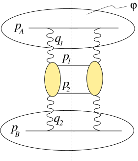
Figure 1: Production of $q\bar{q}$ pair in heavy-ion collisions in $k_{T}$-factorization approach.

The amplitude (47) is rather hard for analytical analysis. We can simplify it in the Regge kinematics $|y_{1}^{*}-y_{2}^{*}|\gg 1$. This limit cannot be used in numerical calculations since quarks tend to be produced at the same rapidity: production of large invariant masses of the $q\bar{q}$ pair is suppressed. However it gives a fair qualitative understanding of the underlying physics. A simple calculation yields

$$\frac{1}{x^{2}y^{2}S^{2}}\,\mathcal{A}(gg\rightarrow ggc\bar{c})\approx\frac{e^{-\Delta y^{*}}}{2m_{1\bot}m_{2\bot}N_{c}}\,\frac{1}{(q_{1}-p_{1})_{\bot}^{2}+m^{2}}\,+\,\mathcal{O}{(e^{-2\Delta y^{*}})}.$$ (14)

In the region of applicability of collinear factorization, $m_{1\bot}\rightarrow\infty$, which at RHIC is the same as $m_{1\bot}\gg Q_{s\mathrm{max}}$, the transverse momenta of gluons are negligible compared to those of produced heavy quarks. Therefore $p_{1\bot}\approx-p_{2\bot}$ and (10) can be written as (we omit numerical factors)

$$\frac{dN^{\mathrm{c\bar{c}}}}{d^{2}p_{\bot 1}\,dy_{1}^{*}dy_{2}^{*}} \propto \frac{\alpha_{s}^{2}e^{-\Delta y^{*}}}{S_{A}}\int^{p_{1\bot}^{2}}\frac{dp_{2\bot}^{2}}{m_{1\bot}m_{2\bot}}\int\,dq_{1\bot}^{2}\frac{1}{N_{c}\,p_{1\bot}^{2}}\frac{A^{2}\,xG_{N}(q_{1\bot}^{2})\,xG_{N}(p_{2\bot}^{2})}{q_{1\bot}^{2}\,p_{2\bot}^{2}}$$ (15)

$$\sim \frac{\alpha_{s}^{2}\,A^{2}\,e^{-\Delta y^{*}}(xG_{N}(p_{1\bot}^{2}))^{2}}{N_{c}\,S_{A}\,p_{1\bot}^{4}}\,\sim\,N_{\mathrm{coll}},$$

where clearly $p_{1\bot}^{2}\gg m^{2}$. Note that the exponential suppression at large $\Delta y^{*}$ of the heavy quark amplitude as compared to the $gg\rightarrow gggg$ [36] is because $t$-channel quark carries spin $1/2$.

At large rapidities there is a kinematic region such that $Q_{s\mathrm{min}}\ll m_{1\bot}\ll Q_{s\mathrm{max}}$. In this case one of the nuclear wave functions is in the saturation whereas another one is not. In general transverse momenta of quarks are no longer equal and point back-to-back. Thus in the limit $p_{1\bot}^{2}\gg p_{2\bot}^{2}$ the quark multiplicity reads

$$\frac{dN^{\mathrm{c\bar{c}}}}{d^{2}p_{\bot 1}\,dy_{1}^{*}dy_{2}^{*}} \propto \frac{\alpha_{s}^{2}e^{-\Delta y^{*}}}{S_{A}}\int\frac{dp_{2\bot}^{2}}{m_{1\bot}m_{2\bot}}\int^{Q_{s\mathrm{max}}^{2}}\,dq_{1\bot}^{2}\frac{1}{N_{c}\,p_{1\bot}^{2}}\frac{S_{A}\,Q_{s\mathrm{min}}^{2}}{q_{1\bot}^{2}}\,\frac{S_{A}}{\alpha_{s}}$$ (16)

$$\sim \frac{1}{N_{c}}\frac{e^{-\Delta y^{*}}\,S_{A}\,Q_{s\mathrm{min}}^{2}}{p_{1\bot}^{2}}\,\ln\frac{Q_{s\mathrm{max}}^{2}}{Q_{s\mathrm{min}}^{2}}\,\sim\,N_{\mathrm{part}}\,\ln\frac{Q_{s\mathrm{max}}^{2}}{Q_{s\mathrm{min}}^{2}}.$$

Please, note that here $Q^{2}_{s\mathrm{min}}\sim\alpha_{s}A/S_{A}$.

Finally, there is a region where both nuclei are in saturation $m_{1\bot}\ll Q_{s\mathrm{min}}$. We have

$$\frac{dN^{\mathrm{c\bar{c}}}}{d^{2}p_{\bot 1}\,dy_{1}^{*}dy_{2}^{*}} \propto \frac{\alpha_{s}^{2}e^{-\Delta y^{*}}}{S_{A}}\int\frac{dp_{2\bot}^{2}}{m_{1\bot}m_{2\bot}}\int^{Q_{s\mathrm{min}}^{2}}\,dq_{1\bot}^{2}\frac{1}{N_{c}\,p_{1\bot}^{2}}\frac{S_{A}^{2}}{\alpha_{s}^{2}}$$ (17)

$$\sim \frac{1}{N_{c}}\frac{e^{-\Delta y^{*}}\,S_{A}\,Q_{s\mathrm{min}}^{2}}{p_{1\bot}^{2}}\,\sim\,N_{\mathrm{part}}.$$

Consider now the total multiplicity of heavy quark pairs produced in heavy ion collisions per unit rapidity, $dN^{\mathrm{c\bar{c}}}/dy_{1}^{*}dy_{2}^{*}$. At RHIC in the kinematic region $|y^{*}|{{}_{\displaystyle{<}}\atop\displaystyle{\sim}}1$ we have $Q_{s}^{2}(y^{*}=0)\simeq 1-2$ GeV². Since $m\simeq 1.2-1.9$ GeV [37] the transverse size of charmed quark $1/m$ is too small to feel saturation in either one of the nuclei and set $N_{\mathrm{part}}$ scaling. The parametric dependence of the total multiplicity of heavy quark pairs is (see (15))

$$\frac{dN^{\mathrm{c\bar{c}}}}{dy_{1}^{*}dy_{2}^{*}}\,\sim\,\frac{\alpha_{s}^{2}A^{2}}{S_{A}}\sim N_{\mathrm{coll}},\quad y^{*}\simeq 0,\quad\mathrm{RHIC}.$$ (18)

Nevertheless, the $k_{T}$-factorization result for total multiplicity is numerically different from the parton model one: since in $k_{T}$-factorization spectrum is harder we get larger total cross section.

Note, that since at RHIC $Q_{s}\sim m$ the variation of the saturation scale with rapidity becomes essential. Variation of $Q_{s}$ with rapidity stems from the fact that the saturation scale is proportional to the gluon density in the transverse plane of nucleus, which in turn is proportional to the gluon structure function $xG(x,k_{\bot}^{2})$. Since $xG(x,k_{\bot}^{2})$ is increasing function of rapidity $y^{*}=\ln(1/x)$ we conclude that $Q_{s}$ grows with $y^{*}$ defined with respect to the rapidity of the nucleus in a given reference frame. Therefore, relation between saturation scales of each nucleus and the quark mass are different at different rapidities $y^{*}$. If we consider quarks produced at $|y^{*}|\gg 1$ (but still not in hadronization region), then one of the nuclei is in saturation while another one is not. In that case we estimate using (16)

$$\frac{dN^{\mathrm{c\bar{c}}}}{dy_{1}^{*}dy_{2}^{*}}\,\sim\,\alpha_{s}A\sim N_{\mathrm{part}},\quad|y^{*}|\gg 1,\quad\mathrm{RHIC,\;LHC}.$$ (19)

In $p(d)A$ collisions, we expect that in the deuteron fragmentation region and for sufficiently central events, the scaling will be

$$\frac{dN^{\mathrm{c\bar{c}}}}{dy_{1}^{*}dy_{2}^{*}}\,\sim\sqrt{N_{\mathrm{part}}^{A}},\quad|y^{*}|\gg 1,\quad\mathrm{RHIC,\;LHC}.$$ (20)

In the next section we will quantify the kinematical region at which the transition to the new scaling will take place at RHIC.

At LHC energies the situation is different. We expect that the saturation scale in the midrapidity region will be much larger than the charmed quark mass. As the result both nuclei will be in the saturation. By (17) we get

$$\frac{dN^{\mathrm{c\bar{c}}}}{dy_{1}^{*}dy_{2}^{*}}\,\sim\,\alpha_{s}^{0}A\sim N_{\mathrm{part}},\quad y^{*}\simeq 0,\quad\mathrm{LHC},$$ (21)

whereas far from midrapidity one of the nuclei is not in saturation and we can use (19). Note that from (11),(12) and (36) it follows that the ratio between the largest and the smallest saturation scales is

$$\frac{Q^{2}_{s\mathrm{max}}}{Q^{2}_{s\mathrm{min}}}\,\simeq\,e^{\lambda(|y_{1}^{*}|+|y_{2}^{*}|)}.$$ (22)

This ratio is much larger than unity when at least one of the quarks is produced at $|y^{*}|\gg 1$ although in most cases quarks are produced at $|y_{1}^{*}-y_{2}^{*}|{{}_{\displaystyle{<}}\atop\displaystyle{\sim}}1$ since otherwise the amplitude is exponentially suppressed (see (14)).

3 Open charm production in $AA$ and $dA$ collisions

3.1 A model for unintegrated gluon distribution

To proceed further we have to specify the unintegrated gluon distribution of a nucleus $\varphi_{A}(x,\underline{q})$. In principle it is directly related to the forward elastic scattering amplitude, which in turn can be calculated from the nonlinear evolution equations [3, 16]. However, their exact analytical solution is not known. Although recently the progress in obtaining the numerical solution was reported by many authors [38] we prefer to use simple parametrization which catches the most essential details of the solution. In this paper we employ a model for distribution function suggested in [9]. It matches the known analytical expressions in the asymptotic regions [30, 39]. It reads

$$\varphi_{A}(x,q^{2}_{\bot}) = \frac{4\,C_{F}}{2(2\pi)^{2}}\frac{S_{\bot}}{\alpha_{s}}\,d\left(\frac{q^{2}_{\bot}}{Q_{s}^{2}(y^{*})}\right)\,(1-x)^{4}\,\Bigg{[}\theta(Q_{s}^{2}\,-\,q_{\bot}^{2})$$ (23)

$$+\,\left(\frac{Q_{s}^{2}(y^{*})}{q^{2}_{\bot}}\right)^{1.3\,\alpha_{s}}\,I_{0}\left\{\left(\ln\frac{Q_{s}^{2}(y^{*})}{Q_{s}^{2}(y_{0}^{*})}\,\ln\frac{q^{2}_{\bot}}{Q_{s}^{2}(y_{0}^{*})}\right)^{1/2}\right\}\,\theta(q^{2}_{\bot}\,-\,Q_{s}^{2})\Bigg{]}$$

The modified Bessel function $I_{0}$ is a solution of the DGLAP and BFKL equations in the double logarithmic approximation,

$$d(\tau)\,=\,\frac{(2\,\tau\,+\,1)}{\sqrt{4\,\tau\,+\,1}}\,\ln\frac{\sqrt{4\,\tau\,+\,1}+1}{\sqrt{4\,\tau\,+\,1}-1}\,-\,1.$$ (24)

In derivation of (23) the phenomenological parametrization of anomalous dimension in the Mellin moment variable $\omega$ was used [40].

$$\gamma(\omega)\,=\,\alpha_{s}\,\left(\frac{1}{\omega}\,-\,1\right).$$ (25)

The first term in the right-hand-side of (25) is the leading order contribution to the anomalous dimension of the DGLAP and BFKL equations in the double-logarithmic approximation. The second term is the phenomenological correction which imposes momentum conservation $\gamma(1)=0$ and describes DIS data well. We also imposed the correct large $x$ behavior on $\varphi_{A}$ by multiplying it by a factor $(1-x)^{4}$.

Let us consider the unintegrated gluon distribution in various kinematic regions. First, consider a perturbative regime in which the collinear factorization is valid $q_{\bot}\gg k_{\mathrm{geom}}(y^{*})$, see (5) and (9). Performing expansion in the exponent of the Bessel function in this regime, using its well-known asymptotic behavior $I_{0}(z)\approx e^{z}$ up to a slowly varying logarithmic factors and expanding in (24) $d(\tau)\approx Q_{s}^{2}(y^{*})/q^{2}_{\bot}$ we get

$$\varphi_{A}(x,q^{2}_{\bot}) \approx \frac{4\,C_{F}}{2(2\pi)^{2}}\frac{S_{A}}{\alpha_{s}}\,\frac{Q_{s}^{2}(y_{0}^{*})}{q^{2}_{\bot}}\left(\frac{Q_{s}^{2}(y^{*})}{q^{2}_{\bot}}\right)^{1.3\alpha_{s}}$$ (26)

$$\times\exp\left\{\left(\ln\frac{Q_{s}^{2}(y^{*})}{Q_{s}^{2}(y_{0}^{*})}\,\ln\frac{q^{2}_{\bot}}{Q_{s}^{2}(y_{0}^{*})}\right)^{1/2}\right\}\,(1-x)^{4}.$$

Next, when the typical parton momentum in the heavy-ion wave function approaches the saturation scale $Q_{s}(y){{}_{\displaystyle{<}}\atop\displaystyle{\sim}}\,q_{\bot}\ll k_{\mathrm{geom}}(y)$ one can expand the Bessel function as [9]:

$$\exp\left\{\left(\ln\frac{Q_{s}^{2}(y^{*})}{Q_{s}^{2}(y_{0}^{*})}\,\ln\frac{q^{2}_{\bot}}{Q_{s}^{2}(y_{0}^{*})}\right)^{1/2}\,-\,\ln\frac{q^{2}_{\bot}}{Q_{s}^{2}(y_{0}^{*})}\right\}\,\approx\,(Q_{s}^{2}(y^{*})/q^{2}_{\bot})^{1/2},$$ (27)

which yields

$$\varphi_{A}(x,\underline{q}^{2})\,\approx\,\frac{4\,C_{F}}{2(2\pi)^{2}}\frac{S_{\bot}}{\alpha_{s}}\,\left(\frac{Q_{s}^{2}(y^{*})}{q^{2}_{\bot}}\right)^{1.3\alpha_{s}\,+\,1/2}\,(1-x)^{4}.$$ (28)

Note that the anomalous dimension is $\gamma=1/2+\mathcal{O}{(\alpha_{s})}$ as desired. Finally, in the saturation region $q_{\bot}<Q_{s}(y)$ the unintegrated gluon distribution reads

$$\varphi_{A}(x,\underline{q}^{2})\,\approx\,\frac{4\,C_{F}}{2(2\pi)^{2}}\frac{S_{\bot}}{\alpha_{s}}\,\ln(Q_{s}^{2}/q_{\bot}^{2})\,(1-x)^{4}.$$ (29)

This expression coincides with the formula for the unintegrated gluon distribution in the saturation regime in the quasi-classical approximation [24]. Actually, it also holds beyond the quasi-classical approximation. Indeed, $\varphi_{A}(x,\underline{q}^{2})$ can be expressed via the gluon dipole forward scattering amplitude $N_{G}(x,\underline{r})$ as [29, 24]

$$\varphi_{A}(x,\underline{q}^{2})\,=\,\frac{4\,C_{F}\,S_{A}}{\alpha_{s}(2\pi)^{2}}\int_{0}^{\infty}dr\,r\,J_{0}(kr)\frac{1}{r^{2}}\,N_{G}(x,\underline{r}^{2}),$$ (30)

where $r$ is the dipole transverse size. As was argued in [30], the forward scattering amplitude in the momentum space at $x\rightarrow 0$ and $q$ fixed is

$$N(x,\underline{q})\,=\,\ln(Q_{s}/q).$$ (31)

In the configuration space we have

$$N(x,\underline{r})\,=\,r^{2}\int_{0}^{Q_{s}}dk\,k\,J_{0}(kr)\,\ln(Q_{s}/k)\,=\,1\,-\,J_{0}(Q_{s}r).$$ (32)

Using the unitarity constraint $N_{G}=2N-N^{2}$ and (30) we derive

$$\varphi_{A}(x,\underline{q}^{2}) = \frac{4\,C_{F}\,S_{A}}{\alpha_{s}\,(2\pi)^{2}}\,\int_{0}^{\infty}\frac{dr}{r}J_{0}(qr)\left(1\,-\,J_{0}^{2}(Q_{s}r)\right)$$ (33)

$$= \frac{4\,C_{F}\,S_{A}}{\alpha_{s}\,2\,(2\pi)^{2}}\,\ln(Q_{s}^{2}/\underline{q}^{2})\,+\mathcal{O}(q/Q_{s}),$$ (34)

which coincides with (29).

Dependence of the saturation scale on energy is known in the double-logarithmic approximation [30, 39]. It was shown in [41] that the photon structure function in the DIS in the whole kinematic region $x<0.01$ can be described by simple Glauber-like parametrization of the gluon distribution with the following saturation scale

$$Q_{s}^{2}(x_{Bj})\,=\,\left(\frac{x_{0}}{x_{Bj}}\right)^{\lambda},$$ (35)

where $x_{0}$ and $\lambda$ are a certain empirical constants. In the case of heavy flavor production we substitute for $x_{Bj}$ expressions for $x$ and $y$ from (11) and (12) for each of the nuclei:

$$Q_{s}^{2\,c\bar{c}}(x)\,=\,\left(\frac{x_{0}}{x_{1}+x_{2}}\right)^{\lambda}$$ (36)

and the same for the other nucleus (with $x\leftrightarrow y$). Since $Q_{s}\sim A^{1/3}$ the saturation scales like $N_{\mathrm{part}}^{1/3}$. In Ref. [7] dependence of $Q_{s}$ on $N_{\mathrm{part}}$ was calculated using the Glauber approach. Here we are going to use the result of that calculation and refer the reader to the Ref. [7] for the explicit table.

3.2 Numerical results

Figure 2: Dependence of the charmed meson yield on centrality at midrapidity and pseudorapidity $\eta=2$ for dAu and Au-Au collisions.

We perform numerical calculation of the charmed quark multiplicity spectrum in heavy-ion collisions at RHIC energies using Eqs. (10) and (23). The parameters we use are: charm quark mass $m=1.3$ GeV, the Golec-Biernat–Wüsthoff parameter $\lambda=0.3$, the strong coupling $\alpha_{s}=0.35$ at $q_{T}\leq Q_{s}$ and runs otherwise and $R_{A}=1.2\,\mathrm{fm}\,A^{1/3}$ for the nuclear radius. In Fig. 2 we present results of the calculation at midrapidity and in the forward region in $AA$ and $dA$ collisions at RHIC energy of $\sqrt{s}=200$ GeV as a function of centrality. We observe that at midrapidity quark spectra exhibit $N_{\mathrm{coll}}$ as expected since $Q_{s}(y^{*}=0)\sim m$ whereas at forward rapidities $y^{*}>2$ the $N_{\mathrm{part}}$ and $\sqrt{N_{\mathrm{part}}^{A}}$ scaling is observed for $AA$ and $dA$ collisions, respectively.

We conclude that the effects of multiple rescatterings and anomalous dimension variation do not affect the centrality dependence in the central rapidity region at RHIC energies for the charm quark production. However saturation significantly affects charm production mechanism in the forward rapidity region.

The charmed-meson spectrum can be calculated by plugging the unintegrated gluon distribution (23) into (10) and convolving with the charmed quark fragmentation function $D_{c}^{h}(z)$

$$\frac{d\sigma_{AA}^{\mathrm{hadron}}}{d^{2}p_{1\bot}\,dy_{1}^{*}}\,=\,\int_{0}^{1}dz\,\frac{d\sigma_{AA}^{\mathrm{jet}}}{d^{2}l_{1\bot}\,dy_{1}^{*}}\,\theta\left(z\,-\,\frac{p_{\bot}}{q_{\mathrm{max}}}\right)\,\delta\,(p_{1\bot}^{2}\,-\,z^{2}\,l_{1\bot}^{2})\,D_{c}^{h}(z)\,\frac{1}{z^{2}}$$ (37)

where $q_{\mathrm{max}}=\sqrt{S}/2$. In our calculation we use the Peterson function [42] with $\epsilon=0.043$ [37].

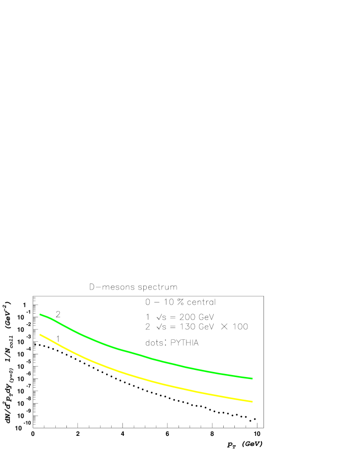
Figure 3: The charmed meson spectrum in heavy-ion collisions at various energies.

Since we determined that the spectrum scales with $N_{\mathrm{coll}}$ in the midrapidity one can easily infer the $dA$ spectrum by scaling it with a corresponding number of binary collisions. The result is then compared to that obtained from PYTHIA event generator with the settings used by PHENIX collaboration [43] (note that PYTHIA is based upon the collinear factorization). In Fig. 3 we observe that PYTHIA spectrum is significantly softer than ours. Therefore, we predict much harder open charm spectrum. Of course, the steepness of the PYTHIA spectrum depends on the intrinsic momentum parameter $k_{0}$. Our spectrum can probably be reproduced by PYTHIA if one takes $k_{0}\simeq Q_{s}\gg\Lambda_{\mathrm{QCD}}$ and fixes the $K$-factor. This large value of intrinsic $k_{T}$ would however signal the breakdown of the collinear factorization approach.

3.3 Distribution in the total momentum of the heavy quark pair

To get further insight into the dynamics of the heavy quark production it can be instructive to directly measure the total momentum of $q\bar{q}$ pair, which has to be equal to zero in the leading order pQCD calculation. Consider the relative motion of the two produced quark momenta in the transverse plane. In the region where collinear factorization is valid the transverse momentum conservation of the process $gg\rightarrow c\bar{c}$ tells us that the transverse momentum distribution must be proportional the delta function $\delta(p_{1\bot}-p_{2\bot})$ in the center-of-mass frame. Due to hadronization the delta function smears out to become a Gaussian of the typical width of the order of $\Lambda^{2}$ independent of the energy and the impact parameter (centrality) of the collision. At momenta $m_{\bot}\leq k_{\mathrm{geom}}\simeq Q_{s}$ the collinear factorization breaks down and we have to use the $k_{T}$-factorization approach. The relevant process is $gg\rightarrow ggc\bar{c}$. Therefore momentum conservation no longer requires that the quark and antiquark momenta be correlated back-to-back $p_{1\bot}=-p_{2\bot}$. In general, the azimuthal distribution of quarks becomes asymmetric and their transverse momentum distribution is disbalanced. The typical difference between the quark momenta is $Q_{s}$ and therefore grows with the energy of collision and centrality. It also become larger for quarks produced far from midrapidity. As wee see, the direct consequence of the saturation of the nuclei wave functions is that the total transverse momentum of the quark–antiquark pair $(p_{1\bot}+p_{2\bot})^{2}$ does not vanish.

Generally, in a given event a number $r$ of $q\bar{q}$ pairs is produced. Let $P_{\bot}$ be the total transverse momentum of all quarks and anti quarks produced in a given event. The averaged total transverse momentum in events with a given $r$ is given by

$$\overline{(P_{\bot}^{2})_{r}} = \int\frac{dN^{\mathrm{c\bar{c}}}}{d^{2}p_{\bot 1}\,dy_{1}^{*}\ldots d^{2}p_{\bot 2r}\,dy_{2r}^{*}}\left(\sum_{i=1}^{2r}p_{i\bot}\right)^{2}\prod_{i=1}^{2r}d^{2}p_{\bot i}\,dy_{i}^{*}$$ (38)

$$\times\left(\int\frac{dN^{\mathrm{c\bar{c}}}}{d^{2}p_{\bot 1}\,dy_{1}^{*}\ldots d^{2}p_{\bot 2r}\,dy_{2r}^{*}}\right)^{-1}$$

With a good accuracy quarks and antiquarks are produced in pairs, thus at this approximation we can write

$$\overline{(P_{\bot}^{2})_{r}} = r\,r^{r-1}\,C^{2}_{2r}\int\frac{dN^{\mathrm{c\bar{c}}}}{d^{2}p_{\bot 1}\,dy_{1}^{*}d^{2}p_{\bot 2}\,dy_{2}^{*}}(p_{1\bot}+p_{2\bot})^{2}\,d^{2}p_{\bot 1}dy_{1}^{*}\,d^{2}p_{\bot 2}\,dy_{2}^{*}\,\frac{1}{r\,C^{2}_{2r}}$$ (39)

$$= r\,\overline{(P_{\bot}^{2})_{1}}.$$

It is convenient to define the event-averaged total transverse momentum of the $c\bar{c}$ pair as follows

$$\langle P_{\bot}^{2}\rangle\,=\,\left\langle\,\frac{1}{r}\,\overline{(P_{\bot}^{2})_{1}}\right\rangle_{\mathrm{all\;events}}.$$ (40)

We can estimate $\langle P_{\bot}^{2}\rangle$ using equations (15),(16),(17) together with (18),(19) and (21). Since in the midrapidity region of RHIC $c\bar{c}$ is produced perturbatively we find

$$\langle P_{\bot}^{2}\rangle\,\simeq\,0,\quad y^{*}\simeq 0,\quad\mathrm{RHIC}.$$ (41)

At larger collision energies, when $Q_{s}(y^{*}=0)\gg m$ both nuclei are saturated and we get (modulo logarithms)

$$\langle P_{\bot}^{2}\rangle\,\simeq\,Q^{2}_{s},\quad y^{*}\simeq 0,\quad\mathrm{LHC}.$$ (42)

At large rapidities, when only one of the nuclei is in saturation we find

$$\langle P_{\bot}^{2}\rangle\,\simeq\,Q^{2}_{s\mathrm{\max}}.\quad|y^{*}|\gg 1,\quad\mathrm{RHIC,\;LHC}.$$ (43)

4 Quenching of the heavy quark spectra
in QCD matter

Our discussion so far has neglected the final state effects. However if hot QCD matter is formed in heavy-ion collisions it could strongly influence the open charm spectrum, similarly to the case of light partons [19, 20, 21]. The energy loss of heavy quarks however is different in one important aspect [44]: since the velocity of heavy quark is smaller than unity, the angular distribution of the gluons emitted in the medium vanishes in the forward direction (“dead cone” effect). Consequently, the collinear singularities disappear, and the sensitivity of the result to the infrared cutoff is greatly diminished which allows for a rigorous perturbative QCD treatment even at small transverse momenta. The resulting energy loss is significantly smaller than for light partons. Recently this issue was also examined in Refs [45].

The medium-modified spectrum can be written as [20, 44]

$$\frac{d\sigma^{\mathrm{med}}}{dp_{\bot}^{2}}\,=\,\frac{d\sigma^{\mathrm{vac}}}{dp_{\bot}^{2}}(p_{\bot})\,Q_{H}(p_{\bot}),$$ (44)

provided that the energy loss is much smaller than $p_{\bot}$. The quantity $d\sigma^{\mathrm{med}}/dp_{\bot}^{2}$ corresponds to the quark spectrum in the vacuum. The quenching factor $Q_{H}(p_{\bot})$ for heavy quarks has been evaluated as [44]

$$Q_{H}(p_{\bot})\simeq\exp\left[-\frac{2\alpha_{s}\,C_{F}}{\sqrt{\pi}}\,L\,\sqrt{\hat{q}\,\frac{\mathcal{L}(p_{\bot})}{p_{\bot}}}\,+\,\frac{16\alpha_{s}}{9\sqrt{3}}\,L\,\left(\frac{\hat{q}\,m^{2}}{m^{2}+p_{\bot}^{2}}\right)^{1/3}\right],$$ (45)

where

$$\mathcal{L}(p_{\bot})\,=\,-\,\frac{d}{d\ln p_{\bot}}\ln\left[\frac{d\sigma^{\mathrm{vac}}}{dp_{T}}(p_{T})\right],$$ (46)

$\hat{q}$ is the transport coefficient and $L$ is the medium size. The charmed meson spectrum in vacuum calculated in the previous section has intrinsic momentum $p_{0}\simeq Q_{s}$. Obviously at $p_{\bot}\gg p_{0}$ we have $\mathcal{L}=\mathrm{const}$ and the quenching factor rapidly approaches unity. However, when $p_{\bot}\ll p_{0}$ we have $\mathcal{L}\propto p_{\bot}$ and the first term in the exponent in (45) stays almost constant. This implies much slower dependence of the quenching factor $Q_{H}(p_{\bot})$ on $p_{T}$. We calculate $\mathcal{L}$ by substituting the quark spectrum into (46). Then, using (45) we calculate the quenching factor for AA collisions (hot matter) and dA collisions (cold medium) which is plotted in Fig. 4.

Figure 4: Quenching factors for hot and cold media $\hat{q}=0.2,\,0.05,\,0.01,\,0.0025$ GeV³. $L=5$ fm.

Note, that the spectrum shape in vacuum in $k_{T}$-factorization is much harder than that in the parton model. Therefore, the fact that we use $k_{T}$-factorization is both qualitatively and quantitatively essential for the result presented in Fig. 4. Even though Fig. 4 exhibits substantial quenching for the values of the gluon transport coefficient that we used, it is still significantly smaller than the quenching factor for the light quarks computed under the same assumptions about the density of the medium.

5 Summary

In conclusion, we have calculated the charmed meson spectrum for heavy ion collisions in the framework of the Color Glass Condensate. We found that at midrapidity the spectrum at RHIC energies scales as $N_{\mathrm{coll}}$, while in the forward region it shows $N_{\mathrm{part}}(\sqrt{N_{\mathrm{part}}^{A}})$ scaling in AA (dA) collisions. Our results are thus different from the predictions based on collinear factorization, even after the leading twist shadowing is included.

Using the explicit form of the charm quark spectrum computed in this approach, we have calculated the quenching factors due to interaction of quarks with hot and cold media. Although at very high $p_{T}$ the quenching factor approaches unity, in a wide region of $2<p_{T}<15$ GeV it stays almost flat. This feature of the quenching factor is a direct consequence of the saturation of the nuclear wave functions which brings in the dimensionful scale $p_{0}\sim Q_{s}$.

We have suggested to determine the saturation scale by measuring the total transverse momentum of charmed mesons produced in a given rapidity interval. We expect that unlike in naive leading order perturbation theory, the total transverse momentum of the pair will not vanish. On the contrary, it will grow with the energy, rapidity and centrality in the same way as the saturation scale.

Acknowledgments

The authors are indebted to Yuri Dokshitzer, Yuri Kovchegov, Eugene Levin, Larry McLerran, Raju Venugopalan and Xin-Nian Wang for fruitful discussions of various aspects of this work. We thank Stefan Kretzer for helpful discussion of heavy quark fragmentation functions, and Zhangbu Xu for providing us with the PYTHIA results for charmed meson spectra. The research of D.K. and K.T. was supported by the U.S. Department of Energy under Grant No. DE-AC02-98CH-10886. The work of K. T. was also sponsored in part by the U.S. Department of Energy under Grant No. DE-FG03-00ER41132.

Appendix

In the Appendix we cite the heavy quark production amplitude $\mathcal{A}(gg\rightarrow ggc\bar{c})$ as given in [26].

$$\mathcal{A}(gg\rightarrow ggc\bar{c})\,=\,\frac{1}{2N_{c}}\,\mathcal{A}^{\mathrm{ab}}\,+\,\frac{N_{c}}{2(N_{c}^{2}-1)}\,\mathcal{A}^{\mathrm{nab}},$$ (47)

where

$$\mathcal{A}^{\mathrm{ab}}\,=\,x^{2}y^{2}S^{2}\left\{\frac{1}{(t-m^{2})(u-m^{2})}\,-\,\frac{1}{q_{1\bot}^{2}q_{2\bot}^{2}}\left[1\,+\,\frac{x_{2}y_{1}S}{t-m^{2}}\,+\,\frac{x_{1}y_{2}S}{u-m^{2}}\right]^{2}\right\},$$ (48)

$$\mathcal{A}^{\mathrm{nab}} = x^{2}y^{2}\left\{S^{2}\left[-\frac{1}{(t-m^{2})(u-m^{2})}\,-\,\frac{1}{s}\left(\frac{1}{t-m^{2}}\,-\,\frac{1}{u-m^{2}}\right)\left(\frac{x_{1}}{x}\,-\,\frac{y_{1}}{y}\right)\right.\right.$$ (49)

$$+\left.\left.\frac{2}{S\,s\,xy}\right]\,+\,\left[\frac{S}{2}\,+\,S^{2}\frac{x_{2}y_{1}}{t-m^{2}}\,-\,\frac{\Delta}{s}\right]\left[\frac{S}{2}\,+\,S^{2}\frac{x_{1}y_{2}}{u-m^{2}}\,+\,\frac{\Delta}{s}\right]\right\}.$$

$$\Delta\,=\,S\left[Sx_{1}y_{2}\,-\,Sx_{2}y_{1}\,+\,q_{1\bot}^{2}\frac{x_{2}}{x}\,-\,q_{2\bot}^{2}\frac{y_{2}}{y}\,+\,\frac{1}{2}(u-t)\,+\,\frac{1}{2}(q_{2\bot}^{2}\,-\,q_{1\bot}^{2})\right]$$ (50)

$$t\,=\,(q_{1}-p_{2})^{2},\quad u\,=\,(q_{1}-p_{1})^{2},\quad s\,\equiv\,\mathcal{M}^{2}\,=\,(p_{1}+p_{2})^{2},$$ (51)

$$q_{1}\,=\,y\,p_{A}\,+\,q_{1\bot},\quad q_{2}\,=\,x\,p_{B}\,+\,q_{2\bot}$$ (52)

$$p_{1,2}\,=\,y_{1,2}\,p_{A}\,+\,x_{1,2}\,p_{B}\,+\,p_{1,2\bot},$$ (53)

where $2p_{A}\cdot p_{B}=S$.

References

- [1] P. Nason, S. Dawson and R. K. Ellis, Nucl. Phys. B 327, 49 (1989) [Erratum-ibid. B 335, 260 (1990)]; P. Nason, S. Dawson and R. K. Ellis, Nucl. Phys. B 303, 607 (1988).
- [2] T. Appelquist and J. Carazzone, Phys. Rev. D 11, 2856 (1975).
- [3] L. V. Gribov, E. M. Levin and M. G. Ryskin, Phys. Rept. 100, 1 (1983).
- [4] A. H. Mueller and J. w. Qiu, Nucl. Phys. B 268, 427 (1986).
- [5] J. P. Blaizot and A. H. Mueller, Nucl. Phys. B 289, 847 (1987).
- [6] L. D. McLerran and R. Venugopalan, Phys. Rev. D 49, 2233 (1994) [arXiv:hep-ph/9309289], Phys. Rev. D 49, 3352 (1994) [arXiv:hep-ph/9311205], Phys. Rev. D 50, 2225 (1994) [arXiv:hep-ph/9402335], Phys. Rev. D 59, 094002 (1999) [arXiv:hep-ph/9809427]. A. Ayala, J. Jalilian-Marian, L. D. McLerran and R. Venugopalan, Phys. Rev. D 53, 458 (1996) [arXiv:hep-ph/9508302].
- [7] D. Kharzeev and M. Nardi, Phys. Lett. B 507, 121 (2001) [arXiv:nucl-th/0012025].
- [8] D. Kharzeev and E. Levin, Phys. Lett. B 523, 79 (2001) [arXiv:nucl-th/0108006].
- [9] D. Kharzeev, E. Levin and L. McLerran, Phys. Lett. B 561, 93 (2003) [arXiv:hep-ph/0210332].
- [10] I. G. Bearden [BRAHMS Collaboration], arXiv:nucl-ex/0207006; I. G. Bearden et al. [BRAHMS Collaboration], Phys. Rev. Lett. 88, 202301 (2002) [arXiv:nucl-ex/0112001]; I. G. Bearden et al. [BRAHMS Collaboration], Phys. Lett. B 523, 227 (2001) [arXiv:nucl-ex/0108016].
- [11] A. Bazilevsky [PHENIX Collaboration], arXiv:nucl-ex/0209025; A. Milov [PHENIX Collaboration], Nucl. Phys. A 698, 171 (2002) [arXiv:nucl-ex/0107006]; K. Adcox et al. [PHENIX Collaboration], Phys. Rev. Lett. 87, 052301 (2001) [arXiv:nucl-ex/0104015]; K. Adcox et al. [PHENIX Collaboration], Phys. Rev. Lett. 86, 3500 (2001) [arXiv:nucl-ex/0012008].
- [12] B. B. Back et al. [PHOBOS Collaboration], Phys. Rev. Lett. 85, 3100 (2000) [arXiv:hep-ex/0007036]; B. B. Back et al. [PHOBOS Collaboration], Phys. Rev. C 65, 061901 (2002) [arXiv:nucl-ex/0201005]; B. B. Back et al. [PHOBOS Collaboration], Phys. Rev. Lett. 88, 022302 (2002) [arXiv:nucl-ex/0108009]; B. B. Back et al. [PHOBOS Collaboration], Phys. Rev. Lett. 87, 102303 (2001) [arXiv:nucl-ex/0106006]; B. B. Back et al. [PHOBOS Collaboration], Phys. Rev. C 65, 031901 (2002) [arXiv:nucl-ex/0105011]. B. B. Back et al. [PHOBOS Collaboration], Phys. Rev. Lett. 85, 3100 (2000) [arXiv:hep-ex/0007036].
- [13] Z. b. Xu [STAR Collaboration], arXiv:nucl-ex/0207019; C. Adler et al. [STAR Collaboration], Phys. Rev. Lett. 87, 112303 (2001) [arXiv:nucl-ex/0106004].
- [14] Y. V. Kovchegov, Phys. Rev. D 54, 5463 (1996) [arXiv:hep-ph/9605446]; Y. V. Kovchegov, Phys. Rev. D 55, 5445 (1997) [arXiv:hep-ph/9701229].
- [15] J. Jalilian-Marian, A. Kovner, A. Leonidov and H. Weigert, Nucl. Phys. B 504, 415 (1997) [arXiv:hep-ph/9701284]. J. Jalilian-Marian, A. Kovner, A. Leonidov and H. Weigert, Phys. Rev. D 59, 014014 (1999) [arXiv:hep-ph/9706377]. J. Jalilian-Marian, A. Kovner, A. Leonidov and H. Weigert, Phys. Rev. D 59, 034007 (1999) [Erratum-ibid. D 59, 099903 (1999)] [arXiv:hep-ph/9807462]. J. Jalilian-Marian, A. Kovner and H. Weigert, Phys. Rev. D 59, 014015 (1999) [arXiv:hep-ph/9709432]. A. Kovner, J. G. Milhano and H. Weigert, Phys. Rev. D 62, 114005 (2000) [arXiv:hep-ph/0004014]. H. Weigert, Nucl. Phys. A 703, 823 (2002) [arXiv:hep-ph/0004044]. E. Iancu, A. Leonidov and L. D. McLerran, Nucl. Phys. A 692, 583 (2001) [arXiv:hep-ph/0011241]. E. Iancu, A. Leonidov and L. D. McLerran, Phys. Lett. B 510, 133 (2001) [arXiv:hep-ph/0102009]. E. Iancu and L. D. McLerran, Phys. Lett. B 510, 145 (2001) [arXiv:hep-ph/0103032]. E. Ferreiro, E. Iancu, A. Leonidov and L. McLerran, Nucl. Phys. A 703, 489 (2002) [arXiv:hep-ph/0109115].
- [16] I. Balitsky, Nucl. Phys. B 463, 99 (1996) [arXiv:hep-ph/9509348]; Y. V. Kovchegov, Phys. Rev. D 60, 034008 (1999) [arXiv:hep-ph/9901281].
- [17] R. Baier, A. H. Mueller, D. Schiff and D. T. Son, Phys. Lett. B 502, 51 (2001) [arXiv:hep-ph/0009237]; R. Baier, A. H. Mueller, D. T. Son and D. Schiff, Nucl. Phys. A 698, 217 (2002); R. Baier, A. H. Mueller, D. Schiff and D. T. Son, Phys. Lett. B 539, 46 (2002) [arXiv:hep-ph/0204211].
- [18] F. Gelis and R. Venugopalan, arXiv:hep-ph/0310090.
- [19] M. Gyulassy and M. Plumer, Phys. Lett. B 243, 432 (1990); M. Gyulassy, M. Plumer, M. Thoma and X. N. Wang, Nucl. Phys. A 538, 37C (1992); X. N. Wang, Z. Huang and I. Sarcevic, Phys. Rev. Lett. 77, 231 (1996) [arXiv:hep-ph/9605213]; X. N. Wang and Z. Huang, Phys. Rev. C 55, 3047 (1997) [arXiv:hep-ph/9701227]; M. Gyulassy, I. Vitev and X. N. Wang, Phys. Rev. Lett. 86, 2537 (2001) [arXiv:nucl-th/0012092]; P. Levai, G. Papp, G. Fai and M. Gyulassy, arXiv:nucl-th/0012017; P. Levai, G. Papp, G. Fai, M. Gyulassy, G. G. Barnafoldi, I. Vitev and Y. Zhang, Nucl. Phys. A 698, 631 (2002) [arXiv:nucl-th/0104035]; I. Vitev and M. Gyulassy, Phys. Rev. C 65, 041902 (2002) [arXiv:nucl-th/0104066]; X. N. Wang and M. Gyulassy, Phys. Rev. Lett. 68, 1480 (1992); M. Gyulassy and X. n. Wang, Nucl. Phys. B 420, 583 (1994) [arXiv:nucl-th/9306003]; X. N. Wang, M. Gyulassy and M. Plumer, Phys. Rev. D 51 (1995) 3436 [arXiv:hep-ph/9408344].
- [20] R. Baier, Y. L. Dokshitzer, S. Peigne and D. Schiff, Phys. Lett. B 345, 277 (1995) [arXiv:hep-ph/9411409]; R. Baier, Y. L. Dokshitzer, A. H. Mueller, S. Peigne and D. Schiff, Nucl. Phys. B 478, 577 (1996) [arXiv:hep-ph/9604327]; R. Baier, Y. L. Dokshitzer, A. H. Mueller, S. Peigne and D. Schiff, Nucl. Phys. B 483, 291 (1997) [arXiv:hep-ph/9607355]; R. Baier, Y. L. Dokshitzer, A. H. Mueller, S. Peigne and D. Schiff, Nucl. Phys. B 484, 265 (1997) [arXiv:hep-ph/9608322]; R. Baier, Y. L. Dokshitzer, A. H. Mueller and D. Schiff, Phys. Rev. C 58, 1706 (1998) [arXiv:hep-ph/9803473]; R. Baier, Y. L. Dokshitzer, A. H. Mueller and D. Schiff, Nucl. Phys. B 531, 403 (1998) [arXiv:hep-ph/9804212]; R. Baier, Y. L. Dokshitzer, A. H. Mueller and D. Schiff, JHEP 0109, 033 (2001) [arXiv:hep-ph/0106347].
- [21] U. A. Wiedemann, Nucl. Phys. A 690, 731 (2001) [arXiv:hep-ph/0008241]; C. A. Salgado and U. A. Wiedemann, arXiv:hep-ph/0310079.
- [22] I. Arsene et al. [BRAHMS Collaboration], suppression,” Phys. Rev. Lett. 91, 072305 (2003) [arXiv:nucl-ex/0307003]; S. S. Adler et al. [PHENIX Collaboration], Phys. Rev. Lett. 91, 072303 (2003) [arXiv:nucl-ex/0306021]. B. B. Back et al. [PHOBOS Collaboration], Phys. Rev. Lett. 91, 072302 (2003) [arXiv:nucl-ex/0306025]. J. Adams et al. [STAR Collaboration], Phys. Rev. Lett. 91, 072304 (2003) [arXiv:nucl-ex/0306024].
- [23] M. Gyulassy and L. D. McLerran, Phys. Rev. C 56, 2219 (1997) [arXiv:nucl-th/9704034].
- [24] D. Kharzeev, Y. V. Kovchegov and K. Tuchin, arXiv:hep-ph/0307037.
- [25] E. M. Levin, M. G. Ryskin, Y. M. Shabelski and A. G. Shuvaev, Sov. J. Nucl. Phys. 53, 657 (1991) [Yad. Fiz. 53, 1059 (1991)]. M. G. Ryskin, Y. M. Shabelski and A. G. Shuvaev, Z. Phys. C 69, 269 (1996) [Yad. Fiz. 59, 521 (1996 PANUE,59,493-500.1996)] [arXiv:hep-ph/9506338].
- [26] S. Catani, M. Ciafaloni and F. Hautmann, Nucl. Phys. B 366, 135 (1991).
- [27] J. C. Collins and R. K. Ellis, Nucl. Phys. B 360, 3 (1991).
- [28] M. G. Ryskin, A. G. Shuvaev and Y. M. Shabelski, Phys. Atom. Nucl. 64, 1995 (2001) [Yad. Fiz. 64, 2080 (2001)] [arXiv:hep-ph/0007238]; P. Hagler, R. Kirschner, A. Schafer, L. Szymanowski and O. Teryaev, Phys. Rev. D 62, 071502 (2000) [arXiv:hep-ph/0002077]; N. P. Zotov, A. V. Lipatov and V. A. Saleev, Phys. Atom. Nucl. 66, 755 (2003) [Yad. Fiz. 66, 786 (2003)]; V. P. Goncalves and M. V. Machado, Eur. Phys. J. C 30, 387 (2003) [arXiv:hep-ph/0305045].
- [29] Y. V. Kovchegov and K. Tuchin, Phys. Rev. D 65, 074026 (2002) [arXiv:hep-ph/0111362].
- [30] E. Levin and K. Tuchin, Nucl. Phys. B 573, 833 (2000) [arXiv:hep-ph/9908317], Nucl. Phys. A 691, 779 (2001) [arXiv:hep-ph/0012167], Nucl. Phys. A 693, 787 (2001) [arXiv:hep-ph/0101275].
- [31] E. Iancu, K. Itakura and L. McLerran, Nucl. Phys. A 708, 327 (2002) [arXiv:hep-ph/0203137], E. Iancu, K. Itakura and L. McLerran, Nucl. Phys. A 724, 181 (2003) [arXiv:hep-ph/0212123].
- [32] A. H. Mueller and D. N. Triantafyllopoulos, Nucl. Phys. B 640, 331 (2002) [arXiv:hep-ph/0205167], A. H. Mueller and D. N. Triantafyllopoulos, double well oscillator,” Nucl. Phys. B 595, 567 (2001) [arXiv:hep-ph/0008266].
- [33] A. M. Stasto, K. Golec-Biernat and J. Kwiecinski, Phys. Rev. Lett. 86, 596 (2001) [arXiv:hep-ph/0007192].
- [34] J. L. Albacete, N. Armesto, A. Kovner, C. A. Salgado and U. A. Wiedemann, arXiv:hep-ph/0307179; R. Baier, A. Kovner and U. A. Wiedemann, Phys. Rev. D 68, 054009 (2003) [arXiv:hep-ph/0305265].
- [35] J. Jalilian-Marian, Y. Nara and R. Venugopalan, arXiv:nucl-th/0307022, and references therein.
- [36] A. Leonidov and D. Ostrovsky, Phys. Rev. D 62, 094009 (2000) [arXiv:hep-ph/9905496].
- [37] K. Hagiwara et al. [Particle Data Group Collaboration], Phys. Rev. D 66, 010001 (2002).
- [38] M. Braun, Eur. Phys. J. C 16, 337 (2000) [arXiv:hep-ph/0001268]. E. Levin and M. Lublinsky, Nucl. Phys. A 696, 833 (2001) [arXiv:hep-ph/0104108]. M. Lublinsky, E. Gotsman, E. Levin and U. Maor, Nucl. Phys. A 696, 851 (2001) [arXiv:hep-ph/0102321]. K. Golec-Biernat, L. Motyka and A. M. Stasto, Phys. Rev. D 65, 074037 (2002) [arXiv:hep-ph/0110325].
- [39] E. Iancu and L. D. McLerran, Phys. Lett. B 510, 145 (2001) [arXiv:hep-ph/0103032]. Y. V. Kovchegov, Phys. Rev. D 54, 5463 (1996) [arXiv:hep-ph/9605446]. A. Krasnitz and R. Venugopalan, Phys. Rev. Lett. 84, 4309 (2000) [arXiv:hep-ph/9909203],
- [40] R. K. Ellis, Z. Kunszt and E. M. Levin, Nucl. Phys. B 420, 517 (1994) [Erratum-ibid. B 433, 498 (1995)].
- [41] K. Golec-Biernat and M. Wusthoff, Phys. Rev. D 59, 014017 (1999) [arXiv:hep-ph/9807513].
- [42] C. Peterson, D. Schlatter, I. Schmitt and P. M. Zerwas, Phys. Rev. D 27, 105 (1983).
- [43] K. Adcox et al. [PHENIX Collaboration], Phys. Rev. Lett. 88, 192303 (2002) [arXiv:nucl-ex/0202002].
- [44] Y. L. Dokshitzer and D. E. Kharzeev, Phys. Lett. B 519, 199 (2001) [arXiv:hep-ph/0106202].
- [45] M. Djordjevic and M. Gyulassy, Phys. Lett. B 560, 37 (2003) [arXiv:nucl-th/0302069]; B. W. Zhang, E. Wang and X. N. Wang, arXiv:nucl-th/0309040; M. Djordjevic and M. Gyulassy, arXiv:nucl-th/0310076.