hep-ph/0310356

CERN–TH/2003-262

UMN–TH–2217/03

TPI–MINN–03/28

Likelihood Analysis of the CMSSM Parameter Space

John Ellis¹, Keith A. Olive², Yudi Santoso² and Vassilis C. Spanos^{2 1}TH Division, CERN, Geneva, Switzerland
²William I. Fine Theoretical Physics Institute,
University of Minnesota, Minneapolis, MN 55455, USA

Abstract

We present a likelihood analysis of the parameter space of the constrained minimal supersymmetric extension of the Standard Model (CMSSM), in which the input scalar masses $m_{0}$ and fermion masses $m_{1/2}$ are each assumed to be universal. We include the full experimental likelihood function from the LEP Higgs search as well as the likelihood from a global precision electroweak fit. We also include the likelihoods for $b\to s\gamma$ decay and (optionally) $g_{\mu}-2$. For each of these inputs, both the experimental and theoretical errors are treated. We include the systematic errors stemming from the uncertainties in $m_{t}$ and $m_{b}$, which are important for delineating the allowed CMSSM parameter space as well as calculating the relic density of supersymmetric particles. We assume that these dominate the cold dark matter density, with a density in the range favoured by WMAP. We display the global likelihood function along cuts in the $(m_{1/2},m_{0})$ planes for $\tan\beta=10$ and both signs of $\mu$, $\tan\beta=35,\mu<0$ and $\tan\beta=50,\mu>0$, which illustrate the relevance of $g_{\mu}-2$ and the uncertainty in $m_{t}$. We also display likelihood contours in the $(m_{1/2},m_{0})$ planes for these values of $\tan\beta$. The likelihood function is generally larger for $\mu>0$ than for $\mu<0$, and smaller in the focus-point region than in the bulk and coannihilation regions, but none of these possibilities can yet be excluded.

CERN–TH/2003-262

October 2003

1 Introduction

Supersymmetry remains one of the best-motivated frameworks for possible physics beyond the Standard Model, and many analyses have been published of the parameter space of the minimal supersymmetric extension of the Standard Model (MSSM). It is often assumed that the soft supersymmetry-breaking mass terms $m_{1/2},m_{0}$ are universal at an input GUT scale, a restriction referred to as the constrained MSSM (CMSSM). In addition to experimental constraints from sparticle and Higgs searches at LEP [1], the measured rate for $b\to s\gamma$ [2] and the value of $g_{\mu}-2$ [3] , the CMSSM parameter space is also restricted by the cosmological density of non-baryonic cold dark matter, $\Omega_{CDM}$ [5, 6, 7, 8]. It is also often assumed that most of $\Omega_{CDM}$ is provided by the lightest supersymmetric particle (LSP), which we presume to be the lightest neutralino $\chi$.

The importance of cold dark matter has recently been supported by the WMAP Collaboration [9, 10], which has established a strong upper limit on hot dark matter in the form of neutrinos. Moreover, the WMAP Collaboration also reports the observation of early reionization when $z\sim 20$ [10], which disfavours models with warm dark matter. Furthermore, the WMAP data greatly restrict the possible range for the density of cold dark matter: $\Omega_{CDM}h^{2}=0.1126^{+0.0081}_{-0.0091}$ (one-$\sigma$ errors). Several recent papers have combined this information with experimental constraints on the CMSSM parameter space [11, 12, 13, 14, 15], assuming that LSPs dominate $\Omega_{CDM}$.

The optimal way to combine these various constraints is via a likelihood analysis, as has been done by some authors both before [16] and after [13] the WMAP data was released. When performing such an analysis, in addition to the formal experimental errors, it is also essential to take into account theoretical errors, which introduce systematic uncertainties that are frequently non-negligible. The main aim of this paper is to present a new likelihood analysis which includes a careful treatment of these errors.

The precision of the WMAP constraint on $\Omega_{CDM}$ selects narrow strips in the CMSSM parameter space, even in the former ‘bulk’ region at low $m_{1/2}$ and $m_{0}$. This narrowing is even more apparent in the coannihilation ‘tail’ of parameter space extending to larger $m_{1/2}$, in the ‘funnels’ due to rapid annihilations through the $A$ and $H$ poles that appear at large $\tan\beta$, and in the focus-point region at large $m_{0}$, close to the boundary of the area where electroweak symmetry breaking remains possible. The experimental and theoretical errors are crucial for estimating the widths of these narrow strips, and also for calculating the likelihood function along cuts across them, as well as for the global likelihood contours we present in the $(m_{1/2},m_{0})$ planes for different choices of $\tan\beta$ and the sign of $\mu$.

In the ‘bulk’ and coannihilation regions, we find that the theoretical uncertainties are relatively small, though they could become dominant if the experimental error in $\Omega_{CDM}h^{2}$ is reduced below 5% some time in the future. However, theoretical uncertainties in the calculation of $m_{h}$ do have an effect on the lower end of the ‘bulk’ region, and these are sensitive to the experimental and theoretical uncertainties in $m_{t}$ and (at large $\tan\beta$) also $m_{b}$. The theoretical errors due to the current uncertainties in $m_{b}$ and $m_{t}$ are dominant in the ‘funnel’ and ‘focus-point’ regions, respectively. These sensitivities may explain some of the discrepancies between the results of different codes for calculating the supersymmetric relic density, which are particularly apparent in these regions. These sensitivities imply that results depend on the treatment of higher-order effects, for which there are not always unique prescriptions.

With our treatment of these uncertainties, we find that the half-plane with $\mu>0$ is generally favoured over that with $\mu<0$, and that, within each half-plane, the coannihilation region of the CMSSM parameter space is generally favoured over the focus-point region , but these preferences are not strong.

The rest of the paper is organized as follows. In section 2, we discuss the treatment of the various constraints employed to define the global likelihood function. In section 3, we present the profile of the global likelihood function along cuts in the $(m_{1/2},m_{0})$ plane for different choices of $\tan\beta$ and the sign of $\mu$. In section 4, we present iso-likelihood contours at certain CLs, obtained by integrating the likelihood function. Finally, in section 5, we summarize our findings and suggest directions for future analyses of this type.

2 Constraints on the CMSSM Parameter Space

2.1 Particle Searches

We first discuss the implementation of the accelerator constraints on CMSSM particle masses. Previous studies have shown that the LEP limits on the masses of sparticles such as the selectron and chargino constrain the CMSSM parameter space much less than the LEP Higgs limit and $b\to s\gamma$ (see, e.g., [7, 17]). As we have discussed previously, in the CMSSM parameter regions of interest, the LEP Higgs constraint reduces essentially to that on the Standard Model Higgs boson [17]. This is often implemented as the 95% confidence-level lower limit $m_{h}>114.4$ GeV [1]. However, here we use the full likelihood function for the LEP Higgs search, as released by the LEP Higgs Working Group. This includes the small enhancement in the likelihood just beyond the formal limit due to the LEP Higgs signal reported late in 2000. This was re-evaluated most recently in [1], and cannot be regarded as significant evidence for a light Higgs boson. We have also taken into account the indirect information on $m_{h}$ provided by a global fit to the precision electroweak data. The likelihood function from this indirect source does not vary rapidly over the range of Higgs masses found in the CMSSM, but we include this contribution with the aim of completeness.

The interpretation of the combined Higgs likelihood, ${\cal L}_{exp}$, in the $(m_{1/2},m_{0})$ plane depends on uncertainties in the theoretical calculation of $m_{h}$. These include the experimental error in $m_{t}$ and (particularly at large $\tan\beta$) $m_{b}$, and theoretical uncertainties associated with higher-order corrections to $m_{h}$. Our default assumptions are that $m_{t}=175\pm 5$ GeV for the pole mass, and $m_{b}=4.25\pm 0.25$ GeV for the running $\overline{MS}$ mass evaluated at $m_{b}$ itself. The theoretical uncertainty in $m_{h}$, $\sigma_{th}$, is dominated by the experimental uncertainties in $m_{t,b}$, which are treated as uncorrelated Gaussian errors:

$$\sigma_{th}^{2}=\left(\frac{\partial m_{h}}{\partial m_{t}}\right)^{2}\Delta m_{t}^{2}+\left(\frac{\partial m_{h}}{\partial m_{b}}\right)^{2}\Delta m_{b}^{2}\,.$$ (1)

The Higgs mass is calculated using the latest version of FeynHiggs [18]. Typically, we find that $(\partial m_{h}/\partial m_{t})\sim 0.5$, so that $\sigma_{th}$ is roughly 2-3 GeV. Subdominant two-loop contributions as well as higher-order corrections have been shown to contribute much less [19].

The combined experimental likelihood, ${\cal L}_{exp}$, from direct searches at LEP 2 and a global electroweak fit is then convolved with a theoretical likelihood (taken as a Gaussian) with uncertainty given by $\sigma_{th}$ from (1) above. Thus, we define the total Higgs likelihood function, ${\cal L}_{h}$, as

$${\cal L}_{h}(m_{h})={{\cal N}\over{\sqrt{2\pi}\,\sigma_{th}}}\int dm^{\prime}_{h}\,\,{\cal L}_{exp}(m^{\prime}_{h})\,\,e^{-(m^{\prime}_{h}-m_{h})^{2}/2\sigma_{th}^{2}}\,,$$ (2)

where ${\cal N}$ is a factor that normalizes the experimental likelihood distribution.

2.2 $b\to s\gamma$ Decay

The branching ratio for the rare decays $b\to s\gamma$ has been measured by the CLEO, BELLE and BaBar collaborations [2], and we take as the combined value ${\cal{B}}(b\to s\gamma)=(3.54\pm 0.41\pm 0.26)\times 10^{-4}$. The theoretical prediction of $b\to s\gamma$ [20, 21] contains uncertainties which stem from the uncertainties in $m_{b}$, $\alpha_{s}$, the measurement of the semileptonic branching ratio of the $B$ meson as well as the effect of the scale dependence. In particular, the scale dependence of the theoretical prediction arises from the dependence on three scales: the scale where the QCD corrections to the semileptonic decay are calculated and the high and low energy scales, relevant to $b\to s\gamma$ decay. These sources of uncertainty can be combined to determine a total theoretical uncertainty. Finally, the experimental measurement is converted into a Gaussian likelihood and convolved with a theoretical likelihood to determine the total likelihood ${\cal L}_{bsg}$ containing both experimental and theoretical uncertainties [20] .

2.3 Measurement of $g_{\mu}-2$

The interpretation of the BNL measurement of $a_{\mu}\equiv g_{\mu}-2$ [3] is not yet settled. Two updated Standard Model predictions for $a_{\mu}$ have recently been calculated [4]. One is based on $e^{+}e^{-}\to$ hadrons data, incorporating the recent re-evaluation of radiative cross sections by the CMD-2 group:

$$a_{\mu}=(11,659,180.9\pm 7.2\pm 3.5\pm 0.4)\times 10^{-10},$$ (3)

and the second estimate is based on $\tau$ decay data:

$$a_{\mu}=(11,659,195.6\pm 5.8\pm 3.5\pm 0.4)\times 10^{-10},$$ (4)

where, in each case, the first error is due to uncertainties in the hadronic vacuum polarization, the second is due to light-by-light scattering and the third combines higher-order QED and electroweak uncertainties. Comparing these estimates with the experimental value [3], one finds discrepancies

$$\Delta a_{\mu}=(22.1\pm 7.2\pm 3.5\pm 8.0)\times 10^{-10}(1.9~{}\sigma)$$ (5)

and

$$\Delta a_{\mu}=(7.4\pm 5.8\pm 3.5\pm 8.0)\times 10^{-10}(0.7~{}\sigma),$$ (6)

for the $e^{+}e^{-}$ and $\tau$ estimates, respectively, where the second error is from the light-by-light scattering contribution and the last is the experimental error from the BNL measurement.

Based on the $e^{+}e^{-}$ estimate, one would tempted to think there is some hint for new physics beyond the Standard Model. However, the $\tau$ estimate does not confirm this optimistic picture. Awaiting clarification of the discrepancy between the $e^{+}e^{-}$ and $\tau$ data, we calculate the likelihood function for the CMSSM under two hypotheses:

• neglecting any information from $g_{\mu}-2$, which may be unduly pessimistic, and

• taking the $e^{+}e^{-}$ estimate (5) at face value, which may be unduly optimistic.

When including the likelihood for the muon anomalous magnetic moment, $a_{\mu}$, we calculate it combining the experimental and the theoretical uncertainties as follows:

$${\cal L}_{a_{\mu}}=\frac{1}{\sqrt{2\pi}\sigma}e^{-(a_{\mu}^{th}-a_{\mu}^{exp})^{2}/2\sigma^{2}}\,,$$ (7)

where $\sigma^{2}=\sigma_{exp}^{2}+\sigma_{th}^{2}$, with $\sigma_{exp}$ taken from (5) and $\sigma_{th}^{2}$ from (1), replacing $m_{h}$ by $a_{\mu}$.

As is well known, the discrepancy (5) would place significant constraints on the CMSSM parameter space, favouring $\mu>0$, though we do consider both signs of $\mu$. In fact, we find that $\mu>0$ is favoured somewhat, even with the ‘pessimistic’ version (6) of the $g_{\mu}-2$ constraint.

2.4 Density of Cold Dark Matter

As already mentioned, we identify the relic density of LSPs with $\Omega_{CDM}h^{2}$. In addition to the CMSSM parameters, the calculation of $\Omega_{CDM}h^{2}$ involves some parameters of the Standard Model that are poorly known, such as $m_{t}$ and $m_{b}$. The default values and uncertainties we assume for these parameters have been mentioned above. Here we stress that both these parameters should be allowed to run with the effective scale $Q$ at which they contribute to the calculation of the relic density, which is typically $Q\simeq 2m_{\chi}$. This effect is particularly important when treating the rapid-annihilation channels due to $\chi\chi\to A,H\to X\bar{X}$ annihilations, but is non-negligible also in other parts of the CMSSM parameter space.

Specifically, the location of the rapid-annihilation funnel due to $A,H$ Higgs-boson exchange, which appears in the region where $m_{A}\simeq 2m_{\chi}$, depends significantly on the determination of $m_{A}$ [6]. For this determination, the input value of the running $\overline{MS}$ mass of $m_{b}$ is a crucial parameter, and the appearance of the funnels depends noticeably on $m_{b}$ [5, 22]. On the other hand, the exact location of the focus-point region [23] (also known as the hyperbolic branch of radiative symmetry breaking [24]) depends sensitively on $m_{t}$ [25, 22, 7], which dictates the scale of radiative electroweak symmetry breaking [26].

In calculating the likelihood of the CDM density, we follow a similar procedure as for the anomalous magnetic moment of the muon in (1, 7), again taking into account the contribution the uncertainties in $m_{t,b}$. In this case, we take the experimental uncertainty from WMAP [9, 10] and the theoretical uncertainty from (1), replacing $m_{h}$ by $\Omega_{\chi}h^{2}$. We will see that the theoretical uncertainty plays a very significant role in our analysis.

2.5 The Total Likelihood

The total likelihood function is computed by combining all the components described above:

$${\cal L}_{tot}={\cal L}_{h}\times{\cal L}_{bs\gamma}\times{\cal L}_{\Omega_{\chi}h^{2}}\times{\cal L}_{a_{\mu}}$$ (8)

In what follows, we consider the CMSSM parameter space at fixed values of $\tan\beta$ = 10, 35, and 50 with $A_{0}=0$. For $\tan\beta$ = 10 and 35, we compute the likelihood function for both signs of $\mu$, but not for $\tan\beta=50$, since in the case the choice $\mu<0$ does not provide a solution of the RGEs with radiative electroweak symmetry breaking.

The likelihood function in the CMSSM can be considered as a function of two variables, ${\cal L}_{tot}(m_{1/2},m_{0})$, where $m_{1/2}$ and $m_{0}$ are the unified GUT-scale gaugino and scalar masses respectively. When plotting confidence levels as iso-likelihood contours in the corresponding $(m_{1/2},m_{0})$ planes, we normalize likelihood function by setting the volume integral

$$\int{\cal L}_{tot}\,dm_{0}\,dm_{1/2}\;=\;1$$ (9)

for each value of $\tan\beta$, combining where appropriate both signs of $\mu$. We also compare the integrals of the likelihood function over the coannihilation and focus-point regions, and for different values of $\tan\beta$.

For most of the results presented below, we perform the analysis over the range $m_{1/2}=100$ GeV up to 1000 GeV for $\tan\beta=10$ and up to 2 TeV for $\tan\beta$ = 35 and 50. The upper limit on $m_{0}$ is taken to be the limit where solutions for radiative electroweak symmetry breaking are possible and the range includes the focus-point region at large $m_{0}$. We discuss below the sensitivity of our results to the choice of the upper limit on $m_{1/2}$.

3 Widths of Allowed Strips in the CMSSM Parameter Space

We begin by first presenting the global likelihood function along cuts through the $(m_{1/2},m_{0})$ plane, for different choices of $\tan\beta$, the sign of $\mu$ and $m_{1/2}$. These exhibit the relative importance of experimental errors and other uncertainties, as well as the potential impact of the $g_{\mu}-2$ measurement.

We first display in Fig. 1 the likelihood along slices through the CMSSM parameter space for $\tan\beta=10,A_{0}=0,\mu>0,$ and $m_{1/2}=300$ and 800 GeV in the left and right panels, respectively, plotting the likelihood as a function of $m_{0}$ in the neighborhood of the coannihilation region [27]. The solid red curves show the total likelihood function calculated including the uncertainties which stem from the experimental errors in $m_{t}$ and $m_{b}$. The green dashed curves show the likelihood calculated without these uncertainties, i.e., we set $\Delta m_{t}=\Delta m_{b}=0$. We see that these errors have significant effects on the likelihood function. In each panel, the horizontal lines correspond to the 68% confidence level of the respective likelihood function. The likelihood functions shown here include ${\cal L}_{a_{\mu}}$ calculated using $e^{+}e^{-}$ data. For these values of $m_{1/2}$ and $m_{0}$ with $\mu>0$, the constraint from $g_{\mu}-2$ is not very significant. For reference, we present in Table 1 and 2 the values of the likelihood functions corresponding to the 68%, 90%, and 95% CLs for each choice of $\tan\beta$ and $\Delta m_{t}$.

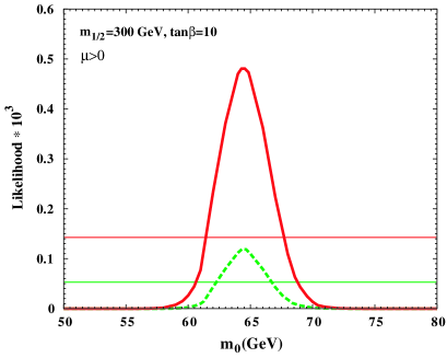
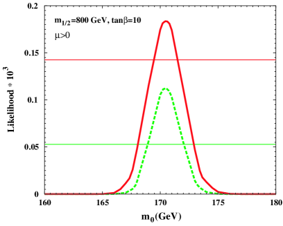
Figure 1: The likelihood function along slices in $m_{0}$ through the CMSSM parameter space for $\tan\beta=10,A_{0}=0,\mu>0$ and $m_{1/2}=300,800$ GeV in the left and right panels, respectively. The solid red curves show the total likelihood function and the green dashed curve is the likelihood function with $\Delta m_{t}=\Delta m_{b}=0$. Both analyses include the $g_{\mu}-2$ likelihood calculated using $e^{+}e^{-}$ data. The horizontal lines show the 68% confidence level of the likelihood function for each case.

Table 1: Likelihood values ($\times 10^{3}$), including $g_{\mu}-2$, for the 68%, 90%, and 95% CLs for different choices of $\tan\beta$ and the uncertainty in $m_{t}$.

$\tan\beta$	CL	$\Delta m_{t}=5$ GeV	$\Delta m_{t}=1$ GeV	$\Delta m_{t}=0.5$ GeV	$\Delta m_{t}=0$ GeV
	68%	0.14	0.13	0.087	0.046
10	90%	3.0 $\times 10^{-3}$	1.4 $\times 10^{-4}$	2.5 $\times 10^{-4}$	0.021
	95%	2.9 $\times 10^{-5}$	6.2 $\times 10^{-5}$	1.1 $\times 10^{-4}$	0.011
	68%	2.2 $\times 10^{-4}$	2.0 $\times 10^{-4}$	2.7 $\times 10^{-4}$	1.1$\times 10^{-3}$
35	90%	2.8 $\times 10^{-5}$	5.0 $\times 10^{-5}$	7.5 $\times 10^{-5}$	1.8$\times 10^{-4}$
	95%	1.1 $\times 10^{-5}$	2.7 $\times 10^{-5}$	3.9 $\times 10^{-5}$	6.8$\times 10^{-5}$
	68%	5.3 $\times 10^{-4}$	5.7 $\times 10^{-4}$	5.4 $\times 10^{-4}$	7.0 $\times 10^{-4}$
50	90%	8.7 $\times 10^{-5}$	7.7 $\times 10^{-5}$	1.0 $\times 10^{-4}$	1.9 $\times 10^{-4}$
	95%	2.3 $\times 10^{-5}$	3.2 $\times 10^{-5}$	4.6 $\times 10^{-5}$	8.2 $\times 10^{-5}$

Table 2: Likelihood values ($\times 10^{3}$), excluding $g_{\mu}-2$, for the 68%, 90%, and 95% CLs for different choices of $\tan\beta$ and the uncertainty in $m_{t}$.

$\tan\beta$	CL	$\Delta m_{t}=5$ GeV	$\Delta m_{t}=1$ GeV	$\Delta m_{t}=0.5$ GeV	$\Delta m_{t}=0$ GeV
	68%	0.059	1.6 $\times 10^{-3}$	9.6 $\times 10^{-4}$	0.052
10	90%	5.6 $\times 10^{-5}$	1.3 $\times 10^{-4}$	2.4 $\times 10^{-4}$	0.024
	95%	4.0 $\times 10^{-5}$	7.9 $\times 10^{-5}$	1.3 $\times 10^{-4}$	0.011
	68%	2.4 $\times 10^{-4}$	1.9 $\times 10^{-4}$	2.4 $\times 10^{-4}$	7.8$\times 10^{-4}$
35	90%	2.3 $\times 10^{-5}$	5.0 $\times 10^{-5}$	7.7 $\times 10^{-5}$	1.6$\times 10^{-4}$
	95%	1.2 $\times 10^{-5}$	2.8 $\times 10^{-5}$	4.0 $\times 10^{-5}$	7.5$\times 10^{-5}$
	68%	3.3 $\times 10^{-4}$	3.5 $\times 10^{-4}$	4.3 $\times 10^{-4}$	6.4 $\times 10^{-4}$
50	90%	4.2 $\times 10^{-5}$	6.4 $\times 10^{-5}$	1.0 $\times 10^{-4}$	1.8 $\times 10^{-4}$
	95%	2.0 $\times 10^{-5}$	3.4 $\times 10^{-5}$	5.0 $\times 10^{-5}$	8.5 $\times 10^{-5}$

When $\mu<0$, the $g_{\mu}-2$ information plays a more important role, as exemplified in Fig. 2, where we show the likelihood in the coannihilation region for $m_{1/2}=800$ GeV. For $m_{1/2}=300$ GeV, the likelihood is severely suppressed (see the discussion below) and we do not show it here.

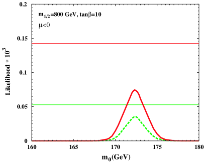
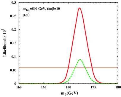
Figure 2: As in Fig. 1 for $\tan\beta=10,A_{0}=0,\mu<0$ and $m_{1/2}=800$ GeV. The $g_{\mu}-2$ constraint is included (excluded) in the left (right) panels. In the right panel the 68% CLs for both cases are incidentally closed to each other.

We now discuss the components of the likelihood function which affect the relative heights along the peaks shown in Fig. 1. In the case $m_{1/2}=300$ GeV, the likelihood increases when the errors in $m_{t}$ and $m_{b}$ are included, due to two dominant effects. 1) The total integrated likelihood is decreased when the errors are turned on (by a factor of $\sim 2$ when $g_{\mu}-2$ is included and by a factor of $\sim 3$ when it is omitted, for $\tan\beta=10$), so the normalization constant, ${\cal N}$, becomes larger, and 2) since $m_{1/2}=300$ GeV corresponds to the lower limit on $m_{1/2}$ due to the experimental bound on the Higgs mass, the Higgs contribution to the likelihood increases when the uncertainties in the heavy quark masses are included. When $m_{1/2}=800$ GeV, it is primarily the normalization effect which results in an overall increase. The Higgs mass contribution at this value of $m_{1/2}$ is essentially ${\cal L}_{h_{exp}}=1$. We remind the reader that the value of the likelihood itself has no meaning. Only the relative likelihoods (for a given normalization) carry any statistical information, which is conveyed here partially by the comparison to the respective 68% CL likelihood values.

In Fig. 3, we extend the previous slices through the CMSSM parameter space to the focus-point region at large $m_{0}$. The solid (red) curve corresponds to the same likelihood function shown by the solid (red) curve in Fig. 1, and the peak at low $m_{0}$ is due to the coannihilation region. The peak at $m_{0}\simeq 2500(4500)$ GeV for $m_{1/2}=300(800)$ GeV is due to the focus-point region . The $g_{\mu}-2$ constraint is not taken into account in the upper two figures of this panel. Also shown in Fig. 3 are the 68%, 90%, and 95% CL lines, corresponding to the iso-likelihood values of the fully integrated likelihood function corresponding to the solid (red) curve. As one can see, one of the effects of the $g_{\mu}-2$ constraint (even at its recently reduced significance) is a suppression of the likelihood function in the focus-point region.

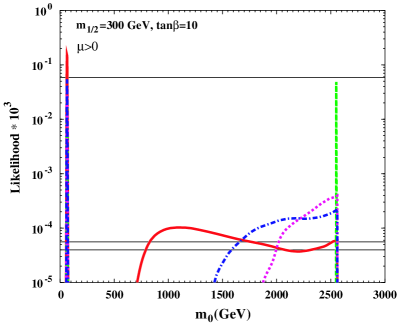
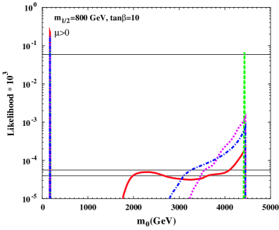
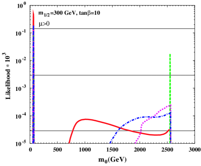
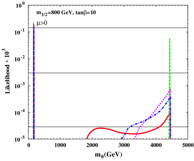
Figure 3: As in Fig. 1, but for slices at fixed $m_{1/2}$ that include also the focus-point region at large $m_{0}$. The red (solid) curves are calculated using the current errors in $m_{t}$ and $m_{b}$, the green dashed curve with no error in $m_{t}$, the violet dotted lines with $\Delta m_{t}=0.5$ GeV, and the blue dashed-dotted lines with $\Delta m_{t}=1$ GeV. In the upper two figures, the $g_{\mu}-2$ constraint has not been applied.

The focus-point peak is suppressed relative to the coannihilation peak at low $m_{0}$ because of the theoretical sensitivity to the experimental uncertainty in the top mass. We recall that the likelihood function is proportional to $\sigma^{-1}$, and that $\sigma$ which scales with $\partial(\Omega_{\chi}h^{2})/\partial m_{t}$, is very large at large $m_{0}$ [22]. This sensitivity is shown in Fig. 4, which plots both $\Omega_{\chi}h^{2}$ and $\partial(\Omega_{\chi}h^{2})/\partial m_{t}$ for the cut corresponding to Fig. 3c. Notice that, for the two values of $m_{0}$ with $\Omega_{\chi}h^{2}\sim 0.1$, corresponding to the coannihilation and focus-point regions, the error due to the uncertainty in $m_{t}$ is far greater in the focus-point region than in the coannihilation region. Thus, even though the exponential in ${\cal L}_{\Omega_{\chi}h^{2}}$ is of order unity near the focus-point region when $\Omega_{\chi}h^{2}\simeq 0.1$, the prefactor is very small due the large uncertainty in the top mass. This accounts for the factor of $\mathrel{\raise 1.29167pt\hbox{$>$\kern-7.5pt\lower 4.30554pt\hbox{$\sim$}}}1000$ suppression seen in Fig. 3 when comparing the two peaks of the solid red curves.

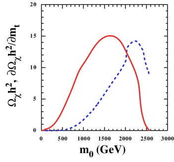
Figure 4: The value of $\Omega_{\chi}h^{2}$ (solid) and $\partial\Omega h^{2}/\partial m_{t}$ (dashed) as functions of $m_{0}$ for $\tan\beta=10,A_{0}=0,\mu>0$ and $m_{1/2}=300$ GeV, corresponding to the slice shown in Fig. 3c.

We note also that there is another broad, low-lying peak at intermediate values of $m_{0}$. This is due to a combination of the effects of $\sigma$ in the prefactor and the exponential. We expect a bump to occur when the Gaussian exponential is of order unity, i.e., $\Omega_{\chi}h^{2}\sim\sqrt{2}\Delta m_{t}\,\partial\Omega_{\chi}h^{2}/\partial m_{t}$. From the solid curve in Fig. 4, we see that $\Omega_{\chi}h^{2}\sim 10$ at large $m_{0}$ for our nominal value $m_{t}$ = 175 GeV, but it varies significantly as one samples the favoured range of $m_{t}$ within its present uncertainty. The competition between the exponential and the prefactor would require a large theoretical uncertainty in $\Omega_{\chi}h^{2}$: $\partial\Omega_{\chi}h^{2}/\partial m_{t}\sim 2$ for $\Delta m_{t}=5$ GeV. From the dashed curve in Fig. 4, we see that this occurs when $m_{0}\sim 1000$ GeV, which is the position of the broad secondary peak in Fig. 3a. At higher $m_{0}$, $\sigma$ continues to grow, and the prefactor suppresses the likelihood function until $\Omega_{\chi}h^{2}$ drops to $\sim 0.1$ in the focus-point region.

As is clear from the above discussion, the impact of the present experimental error in $m_{t}$ is particularly important in this region. This point is further demonstrated by the differences between the curves in each panel, where we decrease ad hoc the experimental uncertainty in $m_{t}$. As $\Delta m_{t}$ is decreased, the intermediate bump blends into the broad focus-point peak. Once again, this can be understood from Fig. 4, where we see that as $\Delta m_{t}$ is decreased, we require a large sensitivity to $m_{t}$ in order to get an increase in ${\cal L}$. This happens at higher $m_{0}$, and thus explains the shift in the intermediate bump to higher $m_{0}$ as $\Delta m_{t}$ decreases. When the uncertainties in $m_{t}$ and $m_{b}$ are set to 0, we obtain a narrow peak in the focus-point region. This is suppressed relative to the coannihilation peak, due to the effect of the $g_{\mu}-2$ contribution to the likelihood.

We can now understand better Tables 1 and 2 for $\tan\beta=10$. For the cases with $\Delta m_{t}\neq 0$ in Table 1 and $\Delta m_{t}=5$ GeV in Table 2, the coannihilation peak is much higher than the focus-point peak, so that the 68% CL (or even the 80% CL) does not include the focus point. To reach the 90% CL, we need to include some part of the focus point, and this explains why the 68% CL is much higher than the 90% CL. The $\Delta m_{t}=1$ GeV case in Table 2 is a peculiar one in which the integral over the coannihilation peak is already around 68% of the total integral and, because the focus point peak is flat and broad, we do not need to change the level much to get the 90% CL. In the cases with $\Delta m_{t}=0$, and also $\Delta m_{t}=0.5$ GeV in Table 2, the focus-point peak is also relatively high and already contributes at the 68% CL. Therefore we do not see an order of magnitude change between the 68% CL and the 90% CL.

As one would expect, the effect of the $g_{\mu}-2$ constraint is more pronounced when $\mu<0$. This is seen in Fig. 5 for the cut with $m_{1/2}=300$ GeV. The most startling feature is the absence of the coannihilation peak at low $m_{0}$ when the $g_{\mu}-2$ constraint is applied. In this case, the focus-point region survives, because the sparticle masses there are large enough for the supersymmetric contribution to $g_{\mu}-2$ to be acceptably small. The broad plateau at intermediate $m_{0}$ is suppressed in this case, and the likelihood does not reach the 95% CL when $\Delta m_{t}=5$ GeV. Another effect of the Higgs mass likelihood can be seen by comparing the coannihilation regions for the two signs of $\mu$ when $m_{1/2}=300$ GeV and the $g_{\mu}-2$ constraint is not applied. Because the Higgs mass constraint is stronger when $\mu<0$ , the coannihilation peak is suppressed when $\mu<0$ relative to its height when $\mu>0$. We note that part of the suppression here is due to the $b\to s\gamma$ constraint, which also favours positive $\mu$.

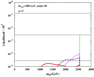
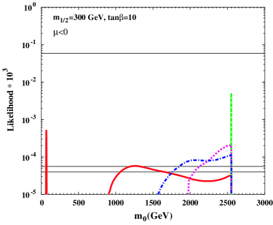
Figure 5: As in Fig. 3, but for $\mu<0$ and $m_{1/2}=300$ GeV, including (excluding) the $g_{\mu}-2$ contribution to the global likelihood in the left (right) panel.

We show in Fig. 6 the likelihood function along cuts in the $(m_{1/2},m_{0})$ plane for $\tan\beta=35,A_{0}=0,\mu<0$ and $m_{1/2}=1000$ GeV (left panels) and $1500$ GeV (right panels). The $g_{\mu}-2$ contribution to the likelihood is included in the bottom panels, but not in the top panels. The line styles are the same as in Fig. 3, and we note that the behaviours in the focus-point regions are qualitatively similar. However, at $m_{0}\sim 1000$ GeV the likelihood function exhibits double-peak structures reflecting the locations of the coannihilation strip and the rapid-annihilation funnels, whose widths depend on the assumed error in $m_{t}$, as can be seen by comparing the different line styles.

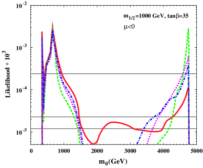
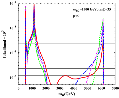
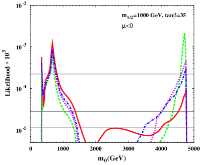
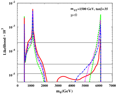
Figure 6: As in Fig. 3 for $\tan\beta=35,A_{0}=0,\mu<0$ and $m_{1/2}=1000,1500$ GeV in the left and right panels. The $g_{\mu}-2$ constraint is included (excluded) in the bottom (top) panels.

Fig. 7 displays the likelihood function along cuts in the $(m_{1/2},m_{0})$ plane for $\tan\beta=50,A_{0}=0,\mu>0$ and $m_{1/2}=800$ GeV (left panels) or $1600$ GeV (right panels). The $g_{\mu}-2$ contribution to the likelihood is included in the bottom panels, but not in the top panels. The line styles are the same as in Fig. 3, and we note that the coannihilation and focus-point regions even link up somewhat below the 95% CL in the case of $m_{0}=800$ GeV, if the present error in $m_{t}$ is assumed, but only if the $g_{\mu}-2$ contribution to the likelihood is discarded. In this case, we can not resolve the difference between the coannihilation and funnel peaks.

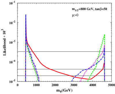
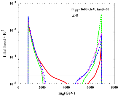
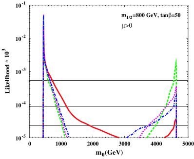
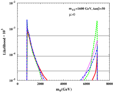
Figure 7: As in Fig. 3 for $\tan\beta=50,A_{0}=0,\mu>0$ and $m_{1/2}=800,1600$ GeV in the left and right panels. The $g_{\mu}-2$ constraint is included (excluded) in the bottom (top) panels.

4 Likelihood Contours in the $(m_{1/2},m_{0})$ Planes

Using the fully normalized likelihood function ${\cal L}_{tot}$ obtained by combining both signs of $\mu$ for each value of $\tan\beta$, we now determine the regions in the $(m_{1/2},m_{0})$ planes which correspond to specific CLs. For a given CL, $x$, an iso-likelihood contour is determined such that the integrated volume of ${\cal L}_{tot}$ within that contour is equal to $x$, when the total volume is normalized to unity. The values of the likelihood corresponding to the displayed contours are tabulated in Table 1 (with $g_{\mu}-2$) and Table 2 (without $g_{\mu}-2$).

Fig. 8 extends the previous analysis to the entire $(m_{1/2},m_{0})$ plane for $\tan\beta=10$ and $A_{0}=0$, including both signs of $\mu$. The darkest (blue), intermediate (red) and lightest (green) shaded regions are, respectively, those where the likelihood is above 68%, above 90%, and above 95%. Overall, the likelihood for $\mu<0$ is less than that for $\mu>0$, even without including any information about $g_{\mu}-2$ due to the Higgs and $b\to s\gamma$ constraints. Only the bulk and coannihilation-tail regions appear above the 68% level, but the focus-point region appears above the 90% level, and so cannot be excluded.

The highly non-Gaussian behaviour of the likelihood shown in Fig. 8 can be understood when comparing this figure to Fig. 3(a,b). At fixed $m_{1/2}$ and for a given CL, portions of the likelihood function above the horizontal lines in 3(a,b) correspond to shaded regions in Fig. 8. The broad low-lying bump or plateau in the likelihood function at intermediate values of $m_{0}$ is now reflected in the extended features seen in Fig. 8. The extent of this plateau is somewhat diminished for $\mu<0$.

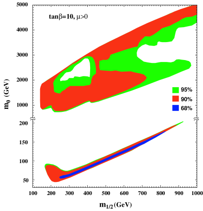
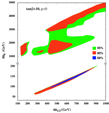
Figure 8: Contours of the likelihood at the 68%, 90% and 95% levels for $\tan\beta=10$, $A_{0}=0$ and $\mu>0$ (left panel) or $\mu<0$ (right panel), calculated using information of $m_{h}$, $b\to s\gamma$ and $\Omega_{CDM}h^{2}$ and the current uncertainties in $m_{t}$ and $m_{b}$, but without using any information about $g_{\mu}-2$.

The bulk region is more apparent in the left panel of Fig. 8 for $\mu>0$ than it would be if the experimental error in $m_{t}$ and the theoretical error in $m_{h}$ were neglected. Fig. 9 complements the previous figures by showing the likelihood functions as they would appear if there were no uncertainty in $m_{t}$, keeping the other inputs the same and using no information about $g_{\mu}-2$. We see that, in this case, both the coannihilation and focus-point strips rise above the 68% CL.

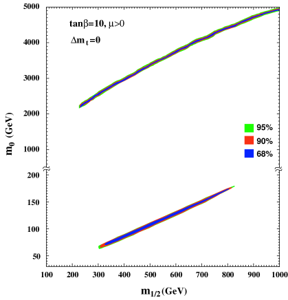
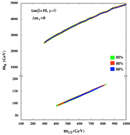
Figure 9: As in Fig. 8 but assuming zero uncertainty in $m_{t}$.

Fig. 10 is also for $\tan\beta=10$ and $A_{0}=0$, including both signs of $\mu$. This time, we include also the $g_{\mu}-2$ likelihood, calculated on the basis of the $e^{+}e^{-}$ annihilation estimate of the Standard Model contribution. This figure represents an extension of Fig. 3(c,d). In this case, very low values of $m_{1/2}$ and $m_{0}$ are disfavoured when $\mu>0$. Furthermore, for $\mu<0$ the likelihood is suppressed and no part of the coannihilation tail is above the 68% CL. In addition, none of the focus point region lies above the 90% CL for either positive or negative $\mu$. However, neither of these can be excluded completely, since there are $\mu<0$ zones within the 90% likelihood contour, and focus-point zones within the 95% likelihood contour.

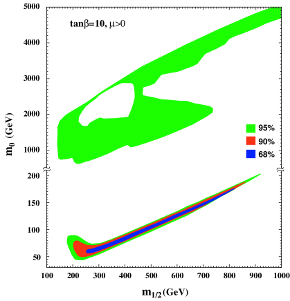
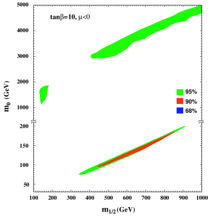
Figure 10: Likelihood contours as in Fig. 8, but also including the information obtained by comparing the experimental measurement of $g_{\mu}-2$ with the Standard Model estimate based on $e^{+}e^{-}$ data.

It is important to note that the results presented thus far are somewhat dependent on the range chosen for $m_{1/2}$, which has so far been restricted for $\tan\beta=10$ to $\leq 1$ TeV. In Fig. 11, we show the the $\tan\beta=10$ plane for $\mu>0$ and $\mu<0$ allowing $m_{1/2}$ up to 2 TeV, including the $g_{\mu}-2$ constraint. Comparing this figure with Fig. 10, we see that a considerable portion of the focus-point region is now above the 90% CL due to the enhanced volume contribution at large $m_{1/2}$.

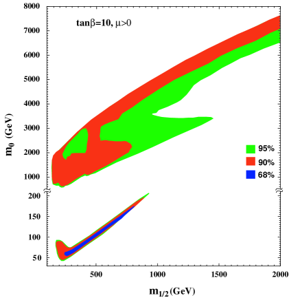
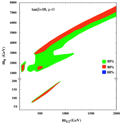
Figure 11: Likelihood contours as in Fig. 10, but extending the range for $m_{1/2}$ up to 2 TeV.

Fig. 12 is for $\tan\beta=35$, $A_{0}=0$ for both $\mu>0$ and $\mu<0$. Fig. 13 includes the $g_{\mu}-2$ likelihood, calculated on the basis of the $e^{+}e^{-}$ annihilation estimate of the Standard Model contribution, which is not included in the previous figure. In this case, regions at small $m_{1/2}$ and $m_{0}$ are disfavoured by the $b\to s\gamma$ constraint, as seen in both figures with $\mu<0$. At larger $m_{1/2}$, the coannihilation region is broadened by a merger with the rapid-annihilation funnel that appears for large $\tan\beta$. The optional $g_{\mu}-2$ constraint would prefer $\mu>0$, and in the $\mu<0$ half-plane it favours larger $m_{1/2}$ and $m_{0}$, as seen when the left and right panels are compared.

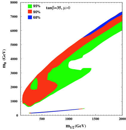
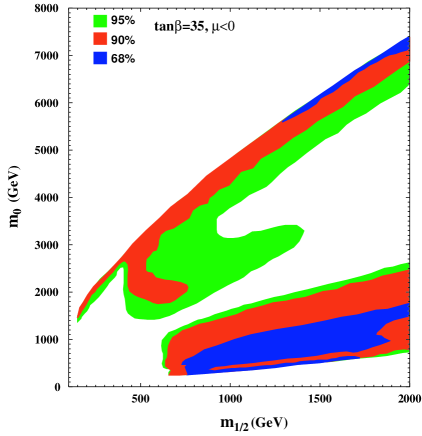
Figure 12: Likelihood contours as in Fig. 8, but for $\tan\beta=35$, $A_{0}=0$ and $\mu>0$ ($\mu<0$) in the left (right) panel, calculated using information of $m_{h}$, $b\to s\gamma$ and $\Omega_{CDM}h^{2}$ and the current uncertainties in $m_{t}$ and $m_{b}$, without the indicative information from $g_{\mu}-2$.

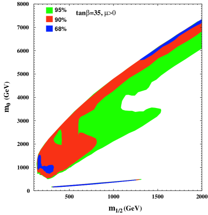
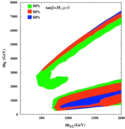
Figure 13: Likelihood contours as in Fig. 12, including the indicative information from $g_{\mu}-2$.

Fig. 14 is for $\tan\beta=50$, $A_{0}=0$ and $\mu>0$. Again, the right panel includes the $g_{\mu}-2$ likelihood, calculated on the basis of the $e^{+}e^{-}$ annihilation estimate of the Standard Model contribution, which is not included in the left panel. In this case, the disfavouring of regions at small $m_{1/2}$ and $m_{0}$ by the $b\to s\gamma$ constraint is less severe than in the case of $\tan\beta=35$ and $\mu<0$, but is still visible in both panels. The coannihilation region is again broadened by a merger with the rapid-annihilation funnel. In the absence of the $g_{\mu}-2$ constraint, both the coannihilation and the focus-point regions feature strips allowed at the 68% CL, and these are linked by a bridge at the 95% CL. However, when the optional $g_{\mu}-2$ constraint is applied, this bridge disappears, the 90% and 95% CL strips in the focus-point region becomes much thinner, and the 68% strip disappears in this region.

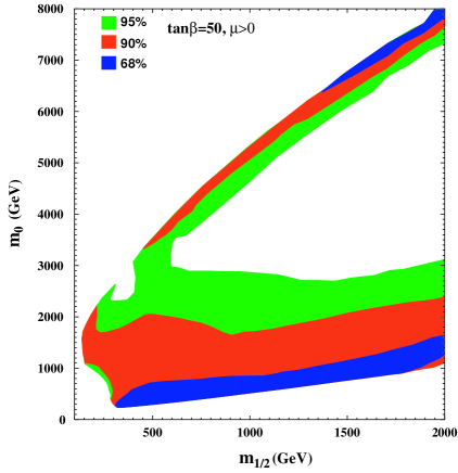
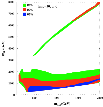
Figure 14: Likelihood contours as in Fig. 12, but for $\tan\beta=50$, $A_{0}=0$ and $\mu>0$, without (left panel) and with (right panel) the indicative information from $g_{\mu}-2$.

5 Summary

We have presented in this paper a new global likelihood analysis of the CMSSM, incorporating the likelihoods contributed by $m_{h}$, $b\to s\gamma$, $\Omega_{CDM}h^{2}$ and (optionally) $g_{\mu}-2$. We have discussed extensively the impacts of the current experimental uncertainties in $m_{t}$ and $m_{b}$, which affect each of $m_{h}$, $b\to s\gamma$ and $\Omega_{CDM}h^{2}$. In particular, the widths of the coannihilation and focus-point strips are sensitive to the uncertainties in $m_{t}$ and $m_{b}$, and a low-lying plateau in the likelihood is found with the present uncertainty $\Delta m_{t}=5$ GeV.

We recall that the absolute values of the likelihood integrals are not in themselves meaningful, but their relative values do carry some information. Generally speaking, the global likelihood function reaches higher values in the coannihilation region than in the focus-point region, as can be seen by comparing the entries with and without parentheses in Table 3. This tendency would have been reversed if the uncertainty in $m_{t}$ had been neglected, as seen in Table 4, but the preference for the coannihilation region is in any case not conclusive.

Table 3 also displays the integrated likelihood function for different values of $\tan\beta$ and the sign of $\mu$, exhibiting a weak general preference for $\mu>0$ if the $g_{\mu}-2$ information is used. If this information is not used, $\mu<0$ is preferred for $\tan\beta=35$, but $\mu>0$ is still preferred for $\tan\beta=10$. There is no significant preference for any value between $\tan\beta=10$ and the upper limits $\mathrel{\hbox to0.0pt{\raise 2.15277pt\hbox{$>$}\hss}{\lower 2.15277pt\hbox{$\sim$}}}35$ and $\mathrel{\hbox to0.0pt{\raise 2.15277pt\hbox{$>$}\hss}{\lower 2.15277pt\hbox{$\sim$}}}50$ where electroweak symmetry breaking ceases to be possible in the CMSSM, though we do find a weak preference for $\tan\beta=50$ and $\mu>0$.

Table 3: Integrals of the global likelihood function integrated over the $(m_{1/2},m_{0})$ planes for various values of $\tan\beta$, in the coannihilation and funnel (focus-point) region. We use the range $m_{1/2}\leq 2\,TeV$, except for the second row of $\tan\beta=10$ case, where the range $m_{1/2}\leq 1\,TeV$ is used.

	incl. $g_{\mu}-2$		without $g_{\mu}-2$
$\tan\beta$	$\mu>0$	$\mu<0$	$\mu>0$	$\mu<0$
10	41.7 (5.9)	2.1 (4.8)	2329 (1052)	1147 (984)
	41.7 (2.9)	2.1 (1.7)	2329 (476)	1147 (387)
35	33.9 (11.6)	25.9 (5.5)	1428 (1596)	8690 (1270)
50	231.9 (6.84)		13096 (1117)

Table 4: As in Table 3, but assuming zero uncertainty in $m_{t}$.

	incl. $g_{\mu}-2$		without $g_{\mu}-2$
$\tan\beta$	$\mu>0$	$\mu<0$	$\mu>0$	$\mu<0$
10	44.9 (69.1)	2.6 (67.7)	2425 (12916)	1485 (13442)
	44.9 (21.4)	2.6 (20.2)	2425 (3922)	1485 (4144)
35	33.5 (90.9)	26.4 (58.3)	1451 (15377)	8837 (12589)
50	195.0 (60.4)		13877 (10188)

In the foreseeable future, the analysis in this paper could be refined with the aid of improved measurements of $m_{t}$ at the Fermilab Tevatron collider, by refined estimates of $m_{b}$, by better determinations of $\Omega_{CDM}h^{2}$ and more experimental and theoretical insight into $g_{\mu}-2$, in particular. One could also consider supplementing our phenomenological analysis with arguments based on naturalness or fine-tuning, which would tend to disfavour larger values of $m_{1/2}$ and $m_{0}$. However, in the absence of such theoretical arguments, our analysis shows that long strips in the coannihilation and focus-point regions cannot be excluded on the basis of present data. The preparations for searches for supersymmetry at future colliders should therefore not be restricted to low values of $m_{1/2}$ and $m_{0}$.

Acknowledgments
We thank Martin Grünewald and Peter Igo-Kemenes for help with the Higgs likelihood, and Geri Ganis for help with the $b\to s\gamma$ likelihood. The work of K.A.O., Y.S., and V.C.S. was supported in part by DOE grant DE–FG02–94ER–40823.

References

-
[1]
LEP Higgs Working Group for Higgs boson searches, OPAL Collaboration,
ALEPH Collaboration, DELPHI Collaboration and L3
Collaboration,
Phys. Lett. B 565 (2003) 61 [arXiv:hep-ex/0306033].
Searches for the neutral Higgs bosons of the MSSM: Preliminary
combined results using LEP data collected at energies up to 209 GeV,
LHWG-NOTE-2001-04, ALEPH-2001-057, DELPHI-2001-114, L3-NOTE-2700,
OPAL-TN-699, arXiv:hep-ex/0107030; LHWG Note/2002-01,
http://lephiggs.web.cern.ch/LEPHIGGS/papers/July2002_SM/index.html. - [2] S. Chen et al. [CLEO Collaboration], Phys. Rev. Lett. 87 (2001) 251807 [arXiv:hep-ex/0108032]; BELLE Collaboration, BELLE-CONF-0135. See also K. Abe et al. [Belle Collaboration], Phys. Lett. B 511 (2001) 151 [arXiv:hep-ex/0103042]; B. Aubert et al. [BaBar Collaboration], arXiv:hep-ex/0207076.
- [3] G. W. Bennett et al. [Muon g-2 Collaboration], Phys. Rev. Lett. 89 (2002) 101804 [Erratum-ibid. 89 (2002) 129903] [arXiv:hep-ex/0208001].
- [4] M. Davier, S. Eidelman, A. Hocker and Z. Zhang, arXiv:hep-ph/0308213.
- [5] J. R. Ellis, T. Falk, G. Ganis, K. A. Olive and M. Srednicki, Phys. Lett. B 510 (2001) 236 [arXiv:hep-ph/0102098].
- [6] A. B. Lahanas and V. C. Spanos, Eur. Phys. J. C 23 (2002) 185 [arXiv:hep-ph/0106345].
- [7] J. R. Ellis, K. A. Olive and Y. Santoso, New J. Phys. 4 (2002) 32 [arXiv:hep-ph/0202110].
- [8] Some additional recent papers include: V. D. Barger and C. Kao, Phys. Lett. B 518 (2001) 117 [arXiv:hep-ph/0106189]; L. Roszkowski, R. Ruiz de Austri and T. Nihei, JHEP 0108 (2001) 024 [arXiv:hep-ph/0106334]; A. Djouadi, M. Drees and J. L. Kneur, JHEP 0108 (2001) 055 [arXiv:hep-ph/0107316]; U. Chattopadhyay, A. Corsetti and P. Nath, Phys. Rev. D 66 (2002) 035003 [arXiv:hep-ph/0201001]; H. Baer, C. Balazs, A. Belyaev, J. K. Mizukoshi, X. Tata and Y. Wang, JHEP 0207 (2002) 050 [arXiv:hep-ph/0205325]; R. Arnowitt and B. Dutta, arXiv:hep-ph/0211417; J. R. Ellis, K. A. Olive, Y. Santoso and V. C. Spanos, Phys. Lett. B 573 (2003) 163 [arXiv:hep-ph/0308075].
- [9] C. L. Bennett et al., Astrophys. J. Suppl. 148 (2003) 1 [arXiv:astro-ph/0302207].
- [10] D. N. Spergel et al., Astrophys. J. Suppl. 148 (2003) 175 [arXiv:astro-ph/0302209].
- [11] J. R. Ellis, K. A. Olive, Y. Santoso and V. C. Spanos, Phys. Lett. B 565 (2003) 176 [arXiv:hep-ph/0303043].
- [12] A. B. Lahanas and D. V. Nanopoulos, Phys. Lett. B 568 (2003) 55 [arXiv:hep-ph/0303130].
- [13] H. Baer and C. Balazs, JCAP 0305 (2003) 006 [arXiv:hep-ph/0303114].
- [14] U. Chattopadhyay, A. Corsetti and P. Nath, Phys. Rev. D 68 (2003) 035005 [arXiv:hep-ph/0303201].
- [15] R. Arnowitt, B. Dutta and B. Hu, arXiv:hep-ph/0310103.
- [16] W. de Boer, M. Huber, C. Sander and D. I. Kazakov, arXiv:hep-ph/0106311.
- [17] M. Battaglia et al., Eur. Phys. J. C 22 (2001) 535 [arXiv:hep-ph/0106204].
- [18] S. Heinemeyer, W. Hollik and G. Weiglein, Comput. Phys. Commun. 124 (2000) 76 [arXiv:hep-ph/9812320]; S. Heinemeyer, W. Hollik and G. Weiglein, Eur. Phys. J. C 9 (1999) 343 [arXiv:hep-ph/9812472].
- [19] S. P. Martin, Phys. Rev. D 67 (2003) 095012 [arXiv:hep-ph/0211366] and talk at SUSY03, Tucson, Arizona (2003).
- [20] C. Degrassi, P. Gambino and G. F. Giudice, JHEP 0012 (2000) 009 [arXiv:hep-ph/0009337], as implemented by P. Gambino and G. Ganis.
- [21] M. Carena, D. Garcia, U. Nierste and C. E. Wagner, Phys. Lett. B 499 (2001) 141 [arXiv:hep-ph/0010003]; D. A. Demir and K. A. Olive, Phys. Rev. D 65 (2002) 034007 [arXiv:hep-ph/0107329]; T. Hurth, arXiv:hep-ph/0106050.
- [22] J. R. Ellis and K. A. Olive, Phys. Lett. B 514 (2001) 114 [arXiv:hep-ph/0105004].
- [23] J. L. Feng, K. T. Matchev and T. Moroi, Phys. Rev. Lett. 84 (2000) 2322 [arXiv:hep-ph/9908309]; J. L. Feng, K. T. Matchev and T. Moroi, Phys. Rev. D 61 (2000) 075005 [arXiv:hep-ph/9909334]; J. L. Feng, K. T. Matchev and F. Wilczek, Phys. Lett. B 482 (2000) 388 [arXiv:hep-ph/0004043].
- [24] K. L. Chan, U. Chattopadhyay and P. Nath, Phys. Rev. D 58 (1998) 096004 [arXiv:hep-ph/9710473].
- [25] A. Romanino and A. Strumia, Phys. Lett. B 487 (2000) 165 [arXiv:hep-ph/9912301].
- [26] A. B. Lahanas, N. E. Mavromatos and D. V. Nanopoulos, arXiv:hep-ph/0308251.
- [27] J. R. Ellis, T. Falk and K. A. Olive, Phys. Lett. B 444 (1998) 367 [arXiv:hep-ph/9810360]; J. R. Ellis, T. Falk, K. A. Olive and M. Srednicki, Astropart. Phys. 13 (2000) 181 [Erratum-ibid. 15 (2001) 413] [arXiv:hep-ph/9905481].