Light front field theory
of quark matter at finite temperature

Abstract

A light front field theory for finite temperature and density is currently being developed. It will be used here to describe the transition region from quark matter to nuclear matter relevant in heavy ion collisions and in the early universe. The energy regime addressed is extremely challenging, both theoretically and experimentally. This is because of the confinement of quarks, the appearance of bound states and correlations, special relativity, and nonlinear phenomena that lead to a change of the vacuum structure of quantum chromodynamics. In the region of the phase transition it eventually leads to a change of the relevant degrees of freedom. We aim at describing this transition from quarks to hadronic degrees of freedom in a unified microscopic approach.

1 Introduction

Lattice calculations of quantum chromodynamics (QCD) give firm evidence that nuclear matter undergoes a phase transition to a plasma state at a certain temperature $T_{c}$ of about 170 to 180 MeV. Calculations have been performed at a chemical potential $\mu=0$. Recent results are for staggered fermions [1, 2] and renormalization group improved Wilson fermions [3]. The low density region reflects, e.g., the scenario during the evolution of the early universe. To achieve information from lattice calculations at small $\mu$ several methods have recently been developed, i.e., multiparameter reweighting [4, 5], Taylor expansion at $\mu\simeq 0$ [6, 7], imaginary $\mu$ [8, 9, 10]. The region of validity is approximately $\mu\lesssim T$ [11]. Effective approaches to QCD indicate an extremely rich phase diagram also for $\mu>T$ [12]. Experimentally the QCD phase diagram is accessible to heavy ion collisions. In particular relativistic heavy ion collision at SPS/CERN and RHIC/BNL explore the region where hadronic degrees of freedom are expected to be dissolved. Some results of RHIC are now available that give hints of a non-hadronic state of matter [13].

On the other hand light-front quantization of QCD can provide a rigorous alternative to lattice QCD [15]. Although the calculational challenge in real QCD of 3+1 dimension seems large (as does lattice QCD) it starts also from the fundamental QCD. The light-front quantization of QCD has the particular advantage that it is completely formulated in physical degrees of freedom. It has emerged as a promising method for solving problems in the strong coupling regime. Light front quantization makes it possible to investigate quantum field theory in a Hamiltonian formulation [14]. This makes it well suited for its application to systems of finite temperature (and density). The relevant field theory has to be quantized on the light front as well, which is presently being developed [16, 17, 18, 19, 20, 21, 22, 23, 24, 25, 26, 27]. I present the light-front field theory at finite temperatures and densities in the next section. For the time being it is applied to the Nambu-Jona-Lasinio model (NJL) model [28, 29] that is a powerful tool to investigate the non-perturbative region of QCD as it exhibits spontaneous breaking of chiral symmetry and the appearance of Goldstone bosons in a transparent way. Finally, going a step further I shall give the general in-medium light cone time ordered Green functions that allow us to treat quark correlations that lead to hadronization.

2 Light front thermal field theory

The four-momentum operator $P^{\mu}$ on the light-front is given by (notation of Ref. [15])

$$P^{\mu}=\int d\omega_{+}\;T^{+\mu}(x),$$ (1)

where $T^{\mu\nu}(x)$ denotes the energy momentum tensor defined through the Lagrangian of the system and $S_{\mu}$ is the quantization surface. The Hamiltonian is given by $P^{-}$. To investigate a grand canonical ensemble we need the number operator,

$$N=\int d\omega_{+}\;j^{+}(x),$$ (2)

where $j^{\nu}(x)$ is the conserved current. These are the necessary ingredients to generalize the covariant partition operator at finite temperature [30, 31, 32] to the light-front. The grand canonical partition operator on the light-front is given by

$$Z_{G}=\exp\left\{\int d\omega_{+}\;[-\beta_{\nu}T^{+\nu}(x)+\alpha J^{+}(x)]\right\},$$ (3)

where $\alpha=\mu/T$, with the Lorentz scalars temperature $T$ and chemical potential $\mu$. The velocity of the medium is given by the time-like vector $u_{\nu}u^{\nu}=1$ [30], and $\beta_{\nu}=u_{\nu}/T$. We choose the medium to be at rest, $u^{\nu}=(u^{-},u^{+},\vec{u}^{\perp})=(1,1,0,0)$. The grand partition operator then becomes

$$Z_{G}=e^{-K/T},\quad K\equiv\frac{1}{2}(P^{-}+P^{+})-\mu N$$ (4)

with $P^{\pm}$ and $N$ defined in (1) and (2). The density operator for a grand canonical ensemble [33, 34] in equilibrium follows

$$\rho_{G}=(\mathrm{Tr}\ e^{-K/T})^{-1}\;e^{-K/T}.$$ (5)

The corresponding Fermi distribution functions of particles $f^{+}\equiv f$ and antiparticles $f^{-}$ are given by

$$f^{\pm}(k^{+},\vec{k}_{\perp})=\left[\exp\left\{\frac{1}{T}\left(\frac{1}{2}k^{-}_{\mathrm{on}}+\frac{1}{2}k^{+}\mp\mu\right)\right\}+1\right]^{-1}$$ (6)

and $k^{-}_{\mathrm{on}}=(\vec{k}_{\perp}^{2}+m^{2})/k^{+}$. This fermionic distribution function (for particles) on the light-front has first been given in [16]. The fermi function for the canonical ensemble can be achieved by simply setting $\mu=0$. This then coincides with the distribution function given recently in Ref. [21] (up to different metric conventions).

The light-front time-ordered Green function for fermions is

$$i{\cal G}_{\alpha\beta}(x-y)=\theta(x^{+}-y^{+})\;\langle\Psi_{\alpha}(x)\bar{\Psi}_{\beta}(y)\rangle-\theta(y^{+}-x^{+})\;\langle\bar{\Psi}_{\beta}(y)\Psi_{\alpha}(x)\rangle.$$ (7)

We note here that the light-cone time-ordered Green function differs from the Feynman propagator $S_{F}$ in the front form by a contact term $\gamma^{+}/2k^{+}$ and therefore coincides with the light-front propagator given previously in Ref. [35]. To evaluate the ensemble average $\langle\dots\rangle=\mathrm{Tr}(\rho_{G}\dots)$ of (7), we utilize the imaginary time formalism [33, 34]. We rotate the light-front time of the Green function to imaginary value. Hence the $k^{-}$-integral is replaced by a sum of light-front Matsubara frequencies $\omega_{n}$ according to [16],

$$\frac{1}{2}k^{-}\rightarrow i\omega_{n}-\frac{1}{2}k^{+}+\mu\equiv\frac{1}{2}k_{n}^{-}\rightarrow\frac{1}{2}z,$$ (8)

where $\omega_{n}=\pi\lambda T$, $\lambda=2n+1$ for fermions [$\lambda=2n$ for bosons]. In the last step we have performed an analytic continuation to the complex plane. For noninteracting Dirac fields the (analytically continued) imaginary time Green function becomes

$$G(z,\overline{k}) = \frac{\gamma k_{\mathrm{on}}+m}{z-k^{-}_{\mathrm{on}}+i\varepsilon}\frac{\theta(k^{+})}{k^{+}}(1-f^{+}(\overline{k}))+\frac{\gamma k_{\mathrm{on}}+m}{z-k^{-}_{\mathrm{on}}-i\varepsilon}\frac{\theta(k^{+})}{k^{+}}f^{+}(\overline{k})$$

$$+\frac{\gamma k_{\mathrm{on}}+m}{z-k^{-}_{\mathrm{on}}+i\varepsilon}\frac{\theta(-k^{+})}{k^{+}}f^{-}(-\overline{k})+\frac{\gamma k_{\mathrm{on}}+m}{z-k^{-}_{\mathrm{on}}-i\varepsilon}\frac{\theta(-k^{+})}{k^{+}}(1-f^{-}(-\overline{k})),$$

where $\overline{k}=(k^{+},\vec{k}_{\perp})$. For equilibrium the imaginary time formalism and the real time formalism are linked by the spectral function [33, 34, 26]. For $\mu=0$ this propagator coincides with that of [26], but differs from that of [21, 25].

3 Spontaneous symmetry breaking and restoration

3.1 NJL model on the light-front

The Nambu-Jona-Lasinio (NJL) originally suggested in [28, 29] has been reviewed in Ref. [36] as a model of quantum chromo dynamics (QCD), where also a generalization to finite temperature and finite chemical potential has been discussed. Its generalization to the light-front including a proper description of spontaneous symmetry breaking, which is not trivial, has been done in Ref. [37], which we use here. The Lagrangian is given by

$${\cal L}=\bar{\psi}(i\gamma\partial-m_{0})\psi+G\left((\bar{\psi}\psi)^{2}+(\bar{\psi}i\gamma_{5}\tau\psi)^{2}\right).$$ (10)

In mean field approximation the gap equation is

$$m=m_{0}-2G\langle\bar{\psi}\psi\rangle=m_{0}+2iG\lambda\int\frac{d^{4}k}{(2\pi)^{4}}\;\mathrm{Tr}S_{F}(k),$$ (11)

where $\lambda=N_{f}N_{c}$ in Hartree and $\lambda=N_{f}N_{c}+{\textstyle\frac{1}{2}}$ in Hartree-Fock approximation, $N_{c}$ ($N_{f}$) is the number of colors (flavors). For the isolated case $S_{F}(k)$ is the Feynman propagator. Taking only the lowest order in $1/N_{c}$ expansion of the 1-body or 2-body operators the light front gap equation can be achieved by a $k^{-}$ integration, where in addition $m_{0}\rightarrow\tilde{m}_{0}$ and $G\rightarrow\tilde{G}$ have to be renormalized to accommodate the expansion. For details see [37]. The propagator to be used in (11) is given in (2). The gap equation becomes

$$m(T,\mu)=\tilde{m}_{0}+2\tilde{G}\lambda\int\frac{dk^{+}d^{2}k_{\perp}}{2k^{+}(2\pi)^{3}}\;4m(T,\mu)(1-f^{+}(k^{+},\vec{k}_{\perp})-f^{-}(k^{+},\vec{k}_{\perp})).$$ (12)

To regularize (12) we require $k^{-}_{\mathrm{on}}+k^{+}<2\Omega$. As a consequence $k^{+}_{1}<k^{+}<k^{+}_{2}$ and

$$\vec{k}^{2}_{\perp} < 2\Omega k^{+}-(k^{+})^{2}-m^{2},$$ (13)

$$k^{+}_{1,2} = \Omega\mp\sqrt{\Omega^{2}-m^{2}}.$$ (14)

For the isolated case this regularization is fully equivalent to the Lepage-Brodsky one and the three-momentum cut-off. For the in medium case this $\Omega$ regularization leads to analytically the same expressions as given in [36] for the instantaneous case [27]. The calculation of the pion mass $m_{\pi}$, the pion decay constant $f_{\pi}$, and the condensate value are also available on the light-front [37].

3.2 Results

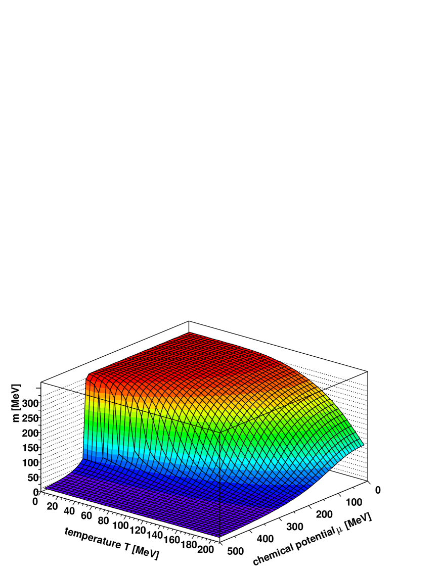
Figure 1: Effective quark mass as a function of temperature and chemical potential. The fall-off is related to the vanishing condensate $\langle\bar{u}u\rangle$, which shows the onset of chiral symmetry restoration. Critical temperature at $\mu=0$ is $T_{c}\simeq 190$ MeV.

Figure 2: Chiral phase transition as defined in [38]. The lower part is the chiral broken phase, whereas the upper part reflects the restored phase.

The model parameters are adjusted to the isolated system. We use the Hartree approximation, i.e. $\lambda=N_{c}N_{f}=6$. Parameter values are chosen to reproduce the pion mass $m_{\pi}=140$ MeV, the decay constant $f_{\pi}=93$ MeV, and to give a constituent quark mass of $m=336$ MeV, i.e. $\tilde{G}=5.51\times 10^{-6}$ MeV, $\tilde{m}_{0}=5.67$ MeV, and $\Omega=714$ MeV. The parameters are reasonably close to the cases used in the review Ref. [36]. The difference between the bare mass $\tilde{m}_{0}$ and the constituent mass is due to the finite condensate, which is $\langle\bar{u}u\rangle^{1/3}=-247$ MeV.

In hot and dense quark matter the surrounding medium leads to a change of the constituent quark mass due to the quasiparticle nature of the quark. The constituent mass as solution of (12) is plotted in Fig. 2 as a function of temperature and chemical potential. The fall-off is related to chiral symmetry restoration, which would be complete for $m_{0}=0$. It is related to the QCD phase transition. For $T\lesssim 60$ MeV the phase transition is first order, which is reflected by the steep change of the constituent mass. To keep close contact with the 3M results we have chosen for the $\Omega$ in-medium regulator mass $\Omega^{2}(T,\mu)=\Lambda_{\mathrm{3M}}^{2}+m^{2}(T,\mu)$ with $\Lambda_{\mathrm{3M}}=630$ MeV fixed for all $T$ and $\mu$.

We define the phase transition to occur at a temperature at which $m(T,\mu)$ is half of the isolated constituent quark mass [38]. The phase diagram is shown in Fig. 2. The line indicates the phase boundary separating the hadronic phase from the quark gluon plasma phase. Results presented in this section are based on an effective interaction in the $q\bar{q}$ channel. They have to be supplemented by the medium dependence of $f_{\pi}$ and $m_{\pi}$ that are currently underway.

4 Few-particle correlations

We are now interested in the $qq$ channel. Since we are going up to the three-particle system, we presently approximate the spin structure. To solve the full three-fermion problem on the light front even for the isolated case is quite a challenge. The spin structure is already rather complex, see e.g. [39]. Therefore the elementary spins are averaged Tr$\gamma=0$ (in the medium) and hence, for the time being, we are only dealing with bose type particles however subject to Fermi-Dirac statistics. Our main focus here is to see how such a three-particle system is dynamically influenced by a medium of finite temperature and density; ultimately, how nucleons are formed in the hot and dense environment of a plasma of quarks and gluons as the temperature and the density becomes smaller and how the relevant degrees of freedom in the Fermi function change as the many-particle system undergoes a change to hadronic degrees of freedom. To this end we need to formulate suitable few-body equations that describe clusters of quarks in a medium. In addition, because of the drastic mass change, see Fig. 2, these equations have to be relativistic ones. The equations derived here are based on a systematic quantum statistical framework formulated on the light front using a cluster expansion for the Green functions. The formalism has been given elsewhere [16]. We repeat here the basics to make a connection to the previous sections. The light-front time ordered cluster Green function is defined by

$$i{\cal G}_{\alpha\beta}(x-y)=\theta(x^{+}-y^{+})\;\langle A_{\alpha}(x)\bar{A}_{\beta}(y)\rangle\mp\theta(y^{+}-x^{+})\;\langle\bar{A}_{\beta}(y)A_{\alpha}(x)\rangle.$$ (15)

where all particles $A_{\alpha}(x)\equiv A_{\alpha}(x^{+},\underline{x})=\Psi_{\alpha_{1}}(x^{+},\underline{x_{1}})\Psi_{\alpha_{2}}(x^{+},\underline{x_{2}})\Psi_{\alpha_{3}}(x^{+},\underline{x_{3}})\dots$ are all taken at the same light front time $x^{+}$ and $\underline{x}=(x_{+},\vec{x}_{\perp})$. The upper (lower) sign stands for fermion (boson) type clusters. Because of the global light-cone time introduced, the dynamical equation for a cluster is equivalent to a Dyson equation with a complicated mass operator that contains an instantaneous part and a memory (or retardation) part. For the time being we neglect the memory term. This is equivalent to a mean field approximation for clusters leading to Faddeev-type three-body equations.

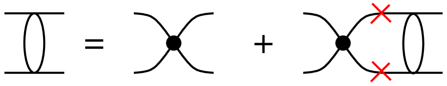
Figure 3: Equation for the two-body $t$-matrix with zero range interaction. The crosses refer to the Pauli-blocking factor.

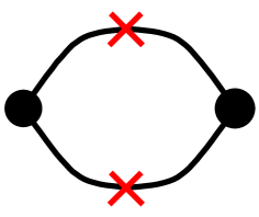
Figure 4: Loop diagram corresponding to the kernel of the integral equation (16).

For a simple zero range interaction the $t$ matrix, Fig. 4, separates and is given by the propagator $t(M_{2})$, i.e.

$$t(M_{2})=\left(i\lambda^{-1}-B(M_{2})\right)^{-1}.$$ (16)

The expression for $B(M_{2})$ is represented by the loop diagram of Fig. 4 and, in the rest system of the two-body system $P^{\mu}=(M_{2},M_{2},\vec{0}_{\perp})$, given by

$$B(M_{2})=-\frac{i}{(2\pi)^{3}}\int\frac{dxd^{2}k_{\perp}}{x(1-x)}\frac{1-f(x,\vec{k}^{2}_{\perp})-f(1-x,\vec{k}_{\perp}^{2})}{M_{2}^{2}-M_{20}^{2}},$$ (17)

where $M_{20}^{2}=(\vec{k}_{\perp}^{2}+m^{2})/x(1-x)$ and $f\equiv f^{-}$ given in (6) with $x=k^{+}/P^{+}_{2}$ where $\overline{P}_{2}=\overline{k}_{1}+\overline{k}_{2}$. For a fermi system there are two important effects occurring due to the blocking factors of (17). One is the dissociation limit (Mott effect) where $M_{2}(T_{d},\mu_{d})=2m(T_{d},\mu_{d})$. Above a certain temperature and density no bound states can be formed. The second effect is related to the appearance of a bose pole in the $t$ matrix. This happens for $M_{2}(T_{c},\mu_{c})=2\mu_{c}$ and defines the critical temperature below which the system becomes unstable and forms a new vacuum consisting of Cooper pairs or a condensate. This is related to superconductivity or superfluidity. In this case for $M_{2}^{2}\rightarrow M^{2}_{02}$, we get

$$f(x,\vec{k}^{2}_{\perp})\Big{|}_{M^{2}_{02}\rightarrow M_{2}^{2}=4\mu^{2}}=f(1-x,\vec{k}_{\perp}^{2})\Big{|}_{M^{2}_{02}\rightarrow M_{2}^{2}=4\mu^{2}}=\frac{1}{2},$$ (18)

i.e. both nominator and denominator of (17) are zero.

The three-particle case is driven by the Fadeev-type in medium equation

$$\Gamma(y,\vec{q}_{\perp})=\frac{i}{(2\pi)^{3}}\ t(M_{2})\int\frac{dxd^{2}k_{\perp}}{x(1-y-x)}\frac{1-f(x,\vec{k}^{2}_{\perp})-f(1-x-y,(\vec{k}+\vec{q})^{2}_{\perp})}{M^{2}_{3}-M_{03}^{2}}\;\Gamma(x,\vec{k}_{\perp}),$$ (19)

where we have introduced vertex functions $\Gamma$ and $t(M_{2})$ given before, and an invariant cut-off $M_{30}^{2}<\Lambda^{2}$. Here the mass of the virtual three-particle state (in the rest system $P^{\mu}=(M_{3},M_{3},\vec{0}_{\perp})$ is

$$M_{03}^{2}=\frac{\vec{k}^{2}_{\perp}+m^{2}}{x}+\frac{\vec{q}^{2}_{\perp}+m^{2}}{y}+\frac{(\vec{k}+\vec{q})^{2}_{\perp}+m^{2}}{1-x-y},$$ (20)

which is the sum of the on-shell minus-components of the three particles. The nucleon scale is introduced by setting $M_{3}=938$ MeV. The isolated quark mass used in these calculations is $m=386$ MeV.

Fig. 6 shows a shaded area that reflect the region where the transition from baryons to quarks (or quark diquarks) occur. The area is defined by use of different regularization masses. The chiral phase transition given before is indicated by the solid line. Fig. 6 shows the possible transition of quark matter to a superconducting phase.

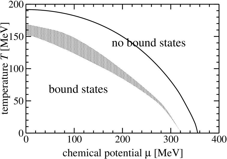
Figure 5: Nucleon dissociation region (shaded area due to different cut-offs). Solid line chiral phase transition of Fig. 2.

Figure 6: Phase diagram supplemented with critical temperature for color superconductivity. Different cut-offs: $\Lambda=4m$ (dot), $\Lambda=6m$ (dash), $\Lambda=8m$ (dash-dot).

5 Conclusion and Outlook

We have given a relativistic formulation of field theory at finite temperatures and densities utilizing the light front form. The proper partition operator (and the statistical operator) have been given for the grand canonical ensemble. The special case of a canonical ensemble is given for $\mu=0$. The resulting Fermi function depends on transverse and also on the $k^{+}$ momentum components. The $k^{+}$ components emerge in a natural way in a covariant approach. As an application we have revisited the NJL low energy model of QCD. We reproduce the phenomenology of the NJL model, in particular the gap-equation and the chiral phase transition. We have further given consistent relativistic three-quark equations valid in a dense medium of finite temperature. We find that the dissociation transition and the critical temperature for the color superconductivity agree qualitatively with results expected from other sources. However, the latter results are by no means final. We have shown that it is possible to write down meaningful consistent equations to solve the relativistic in-medium problem on the light front. The next steps would be to use the NJL model all through to give a consistent picture for the $q\bar{q}$ and the $qq$ channel. Further insight into this just emerging possibilities of treating relativistic many-particle systems on the light front might be provided by other theories, like 1+1 QCD, the Yukawa model, and finally real QCD.

Acknowledgment:

I gratefully acknowledge the fruitful collaboration with S. Mattiello, T. Frederico, and H.J. Weber, who have substantially contributed to the work I had the pleasure to present in this talk. I also thank S. Brodsky for his interest and discussion on this new approach. In particular, I would like to thank the organizers of the workshop for a fruitful and well organized meeting. Work supported by Deutsche Forschungsgemeinschaft, grant BE 1092/10.

References

- [1] C. Bernard et al. [MILC Collaboration], arXiv:hep-lat/0309118 and refs. therein
- [2] F. Karsch, E. Laermann and A. Peikert, Nucl. Phys. B 605 (2001) 579.
- [3] A. Ali Khan et al. [CP-PACS collaboration], Phys. Rev. D 64 (2001) 074510.
- [4] Z. Fodor and S. D. Katz, Phys. Lett. B 534, 87 (2002)].
- [5] Z. Fodor, S. D. Katz and K. K. Szabo, Phys. Lett. B 568, 73 (2003).
- [6] C. R. Allton et al., Phys. Rev. D 66, 074507 (2002).
- [7] C. R. Allton et al., Phys. Rev. D 68, 014507 (2003).
- [8] P. de Forcrand and O. Philipsen, Nucl. Phys. B 642, 290 (2002).
- [9] M. D’Elia and M. P. Lombardo, Phys. Rev. D 67, 014505 (2003).
- [10] P. de Forcrand and O. Philipsen, arXiv:hep-lat/0307020.
- [11] S. D. Katz, arXiv:hep-lat/0310051.
- [12] M. G. Alford, Nucl. Phys. Proc. Suppl. 117 (2003) 65.
- [13] U. W. Heinz, Nucl. Phys. A 721 (2003) 30.
- [14] P. A. Dirac, Rev. Mod. Phys. 21, 392 (1949).
- [15] S. J. Brodsky, H. C. Pauli and S. S. Pinsky, Phys. Rept. 301, 299 (1998), and refs. therein.
- [16] M. Beyer, S. Mattiello, T. Frederico and H. J. Weber, Phys. Lett. B 521, 33 (2001).
- [17] S. Mattiello, M. Beyer, T. Frederico and H. J. Weber, Few Body Syst. 31, 159 (2002).
- [18] S. J. Brodsky, Acta Phys. Polon. B 32, 4013 (2001).
- [19] S. J. Brodsky, Fortsch. Phys. 50, 503 (2002).
- [20] S.J. Brodsky, Nucl. Phys. Proc. Suppl. 108, 327 (2002).
- [21] V. S. Alves, A. Das and S. Perez, Phys. Rev. D 66, 125008 (2002).
- [22] S. Mattiello, M. Beyer, T. Frederico and H. J. Weber, Few Body Syst. Suppl. 14, 379 (2003)
- [23] H. A. Weldon, Phys. Rev. D 67, 085027 (2003).
- [24] H. A. Weldon, Phys. Rev. D 67, 128701 (2003).
- [25] A. Das and X. x. Zhou, arXiv:hep-th/0305097.
- [26] A. N. Kvinikhidze and B. Blankleider, arXiv:hep-th/0305115.
- [27] M. Beyer, S. Mattiello, T. Frederico and H. J. Weber, arXiv:hep-ph/0310222.
- [28] Y. Nambu and G. Jona-Lasinio, Phys. Rev. 122, 345 (1961).
- [29] Y. Nambu and G. Jona-Lasinio, Phys. Rev. 124, 246 (1961).
- [30] W. Israel, Annals Phys. 100, 310 (1976).
- [31] W. Israel, Physics 106A, 204 (1981).
- [32] H. A. Weldon, Phys. Rev. D 26, 1394 (1982).
- [33] L.P.Kadanov and G. Baym, Quantum Statistical Mechanics (Mc Graw-Hill, New York 1962).
- [34] A.L. Fetter, J.D. Walecka, Quantum Theory of Many-Particle Systems (McGraw-Hill, New York 1971) and Dover reprints 2003.
- [35] S.-J. Chang, R.G. Root, and T.-M. Yan, Phys. Rev. D7, 1133 (1973); S.J. Chang and T.-M. Yan, Phys. Rev. D7, 1147 (1973).
- [36] S.P. Klevansky, Rev. Mod. Phys. 64, 649 (1992).
- [37] W. Bentz, T. Hama, T. Matsuki and K. Yazaki, Nucl. Phys. A 651, 143 (1999).
- [38] M. Asakawa and K. Yasaki, Nucl. Phys. A504, 668 (1989).
- [39] M. Beyer, C. Kuhrts and H. J. Weber, Annals Phys. 269, 129 (1998).