Difference of $\tilde{\epsilon}$ and $\epsilon$ in fitting the partameters of CKM matrix.

Abstract

The difference between induced by box diagram value of $\tilde{\epsilon}$ and experimentally measured value of $\epsilon$ is estimated. It appeared to be around $5-10\%$, depending on the values of hadronic matrix elements. With this result, the fit of CKM marix parameters within the SM is performed.

1 Introduction.

It is well known that CP - violation in $K^{0}-\bar{K}^{0}$ mixing is described by the parameter $\tilde{\epsilon}$. Within the SM, this parameter is given by box diagrams. It depends in particular on the CKM matrix elements. On the other hand, the experimentally measured parameters are $\epsilon$ and $\epsilon^{\prime}$. $\epsilon$ and $\epsilon^{\prime}$ enter the measured ratios of decay amplitudes of kaons into $\pi\pi$ states. These amplitudes are superpositions of amplitudes $A(K^{0}\to(\pi\pi)_{I})=A_{I}e^{i\delta_{I}}$ of kaon decays into states with definite isospin $I=0,2$, $A_{I}$ are weak amplitudes, $\delta_{I}$ are strong rescattering phases(see Appendix for details). The parameter $\epsilon$ can be expressed as [1]:

$$\epsilon=\tilde{\epsilon}+i\frac{ImA_{0}}{ReA_{0}}.$$ (1)

Within the SM, $ImA_{0}$ originates from the so-called strong penguin diagrams. Amplitude $A_{2}$ also has an imaginary part which originates from electro-weak penguin diagrams. That is why $ImA_{0}>>ImA_{2}$. The ratio $\displaystyle{\frac{ImA_{0}}{ReA_{0}}}$ is much smaller than $\tilde{\epsilon}$ and when the fit of the CKM matrix parameters is performed, one equates the experimentally measured value of $|\epsilon|$ and theoretical expression for $|\tilde{\epsilon}|$, neglecting the term $\displaystyle{\frac{ImA_{0}}{ReA_{0}}}$, see [2],[3]. In particular it was claimed in [4] that the contribution of $\displaystyle{\frac{ImA_{0}}{ReA_{0}}}$ is ”at most a 2% correction to $\epsilon$”. The aim of the present paper is to take this usually neglected term into account.

In order to estimate the ratio $\displaystyle{\frac{ImA_{0}}{ReA_{0}}}$ we exploit the fact that it enters the expression for $\displaystyle{\frac{\epsilon^{\prime}}{\epsilon}}$[1]:

$$\frac{\epsilon^{\prime}}{\epsilon}=\frac{i}{\sqrt{2}}e^{i(\delta_{2}-\delta_{0})}\frac{1}{\epsilon}\left[\frac{ImA_{2}}{ReA_{0}}-w\frac{ImA_{0}}{ReA_{0}}\right]~{},$$ (2)

where $\displaystyle{w=\frac{ReA_{2}}{ReA_{0}}}$.

The ratio $\displaystyle{\frac{\epsilon^{\prime}}{\epsilon}}$ is experimentally measured and great amount of work was done in order to calculate it(see [5] - [10] and refs. therein). In particular the quantity $\displaystyle{\frac{ImA_{0}}{ReA_{0}}}$ was computed theoretically using different methods. We shall use the results of these computations.

We shall imply the following three step procedure for estimating $\displaystyle{\frac{ImA_{0}}{ReA_{0}}}$.

At first step we neglect $ImA_{0}$. Then $|\tilde{\epsilon}_{theor.}|$ coincides with $|\epsilon_{exp.}|$, and we reproduce the results of [2],[3].

At second step we take into account that $ImA_{0}\neq 0$, but neglect the contribution of EW penguins in Eq.(2). Then we extract the value of $\displaystyle{\frac{ImA_{0}}{ReA_{0}}}$ from experimentally measured quantity $\displaystyle{\frac{\epsilon^{\prime}}{\epsilon}}$ with the help of Eq.(2).

At third step we take into account the contribution of EW penguins: $ImA_{2}\neq 0$. The consequence is that one cannot extract $\displaystyle{\frac{ImA_{0}}{ReA_{0}}}$ from Eq.(2). So one has to use the results of theoretical computation of $\displaystyle{\frac{ImA_{0}}{ReA_{0}}}$.

Finally, we perform a fit of CKM matrix parameters, taking the term $\displaystyle{\frac{ImA_{0}}{ReA_{0}}}$ in Eq.(1) into account and using numerical estimate of it, obtained at step 3.

2 Difference between $\tilde{\epsilon}$ and $\epsilon$.

The quantities $\epsilon$ and $\tilde{\epsilon}$ are related by Eq.(1). Taking into account that the phase of $\tilde{\epsilon}$ is approximately $\frac{\pi}{4}$ [1] (see also Appendix), from Eq.(1) we deduce:

$$|\epsilon|=\left|\tilde{\epsilon}+i\frac{ImA_{0}}{ReA_{0}}\right|=\sqrt{\frac{1}{2}|\tilde{\epsilon}|^{2}+\left(\frac{1}{\sqrt{2}}|\tilde{\epsilon}|+\frac{ImA_{0}}{ReA_{0}}\right)^{2}}.$$ (3)

Thus:

$$|\tilde{\epsilon}|=-\frac{1}{\sqrt{2}}\frac{ImA_{0}}{ReA_{0}}+\sqrt{|\epsilon|^{2}-\frac{1}{2}\left(\frac{ImA_{0}}{ReA_{0}}\right)^{2}}\approx|\epsilon|-\frac{1}{\sqrt{2}}\frac{ImA_{0}}{ReA_{0}}.$$ (4)

The experimentally measured value is [11]:

$$|\epsilon^{exp}|=2.282(17)\times 10^{-3}.$$ (5)

Now we start our procedure of estimating $|\tilde{\epsilon}|$. At first step we neglect $\displaystyle{\frac{ImA_{0}}{ReA_{0}}}$ and obtain:

$$|\tilde{\epsilon}|=|\epsilon^{exp}|=2.282(17)\times 10^{-3}.$$ (6)

This formula is always used in the fits of CKM matrix parameters, see [2],[3].

Second step: We take into account that $ImA_{0}\neq 0$ but neglect $ImA_{2}$. Then Eq.(2) reduces to:

$$\frac{\epsilon^{\prime}}{\epsilon}\approx-\frac{i}{\sqrt{2}}e^{i(\delta_{2}-\delta_{0}-\frac{\pi}{4})}\frac{w}{|\epsilon|}\frac{ImA_{0}}{ReA_{0}}.$$ (7)

Taking into account that $(\delta_{0}-\delta_{2})_{exp}=42\pm 4^{o}$ [12], we obtain the following expression for $\displaystyle{\frac{ImA_{0}}{ReA_{0}}}$:

$$\frac{ImA_{0}}{ReA_{0}}\approx-\frac{\sqrt{2}|\epsilon|}{w}\frac{\epsilon^{\prime}}{\epsilon}.$$ (8)

Substituting experimental values from [11] we get:

$$\frac{\epsilon^{\prime}}{\epsilon}=1.8(4)\times 10^{-3},\quad w=0.045,\quad|\epsilon|=2.282(17)\times 10^{-3}\Longrightarrow$$

$$\frac{ImA_{0}}{ReA_{0}}=-(1.3\pm 0.3)\times 10^{-4}.$$ (9)

In this way we get the following value of $|\tilde{\epsilon}|$, which is the result of the second step:

$$|\tilde{\epsilon}|=2.37(2)\times 10^{-3}.$$ (10)

This number coincides with the value obtained in [13], Eqs.(9.3),(9.4).

Third step: Now let us take into account the presence of EW penguins: $ImA_{2}\neq 0$. Then Eq.(2) does not allow to extract $\displaystyle{\frac{ImA_{0}}{ReA_{0}}}$ from the experimental data and we need explicit theoretical result for $\displaystyle{\frac{ImA_{0}}{ReA_{0}}}$. As announced in the Introduction, such result was obtained in the literature while calculating theoretically $\displaystyle{\frac{\epsilon^{\prime}}{\epsilon}}$.

In order to calculate $\displaystyle{\frac{\epsilon^{\prime}}{\epsilon}}$ from Eq.(2) , one needs theoretical expressions for $ImA_{0}$ and $ImA_{2}$ (the values of $ReA_{0}$, $ReA_{2}$, $|\epsilon|$, $\delta_{0}-\delta_{2}$ and $w$ are well measured experimentally). Short review of the history of $\displaystyle{\frac{\epsilon^{\prime}}{\epsilon}}$ calculation can be found in [10]. The expressions for $ImA_{0}$ and $ImA_{2}$ are usually presented in the following form:

$$ImA_{0}=-\frac{G_{F}}{\sqrt{2}}Im(V_{td}V_{ts}^{*})P^{(0)}(1-\Omega_{IB}),$$

$$ImA_{2}=-\frac{G_{F}}{\sqrt{2}}Im(V_{td}V_{ts}^{*})P^{(2)},$$ (11)

where

$$P^{(I)}=\sum_{i}y_{i}\langle Q_{i}\rangle_{I},\quad I=0,2.$$ (12)

Here $V_{td}$ and $V_{ts}^{*}$ are CKM matrix elements, $G_{F}$ - Fermi constant, $\langle Q_{i}\rangle_{0,2}$ are matrix elements of 4-quark operators responsible for $K\rightarrow\pi\pi$ decays, $y_{i}$ being their Wilson coefficients, $\Omega_{IB}$ introduces a correction due to isospin breaking effects: $\displaystyle{\Omega_{IB}=\frac{1}{w}\frac{(ImA_{2})_{IB}}{ImA_{0}}}$.

From (2) we have:

$$\frac{ImA_{0}}{ReA_{0}}=-\frac{G_{F}}{\sqrt{2}ReA_{0}}Im(V_{td}V_{ts}^{*})P^{(0)}(1-\Omega_{IB}).$$ (13)

This formula contains the CKM matrix elements (which we are going to fit), but for the estimate of the small correction to $|\tilde{\epsilon}|$ we can use mean values from [15]: $Im(V_{td}V_{ts}^{*})=0.000127$. $ReA_{0}$ is well measured experimentally: $ReA_{0}=3.33\times 10^{-7}GeV$. Concerning $P^{(0)}(1-\Omega_{IB})$, we use data from the calculations of $\displaystyle{\frac{\epsilon^{\prime}}{\epsilon}}$ done in [8], which succeed in describing the experimental value of $\displaystyle{\frac{\epsilon^{\prime}}{\epsilon}}$.

Hadronic matrix elements were evaluated in [8] using large $N_{c}$ - expansion. From Table 2 of [8] we find the following range of values (corresponding to the quark condensate value $\left(<\bar{\psi}\psi>\right)^{\frac{1}{3}}=0.240-0.260\,GeV$ at $\mu=2\,GeV$): $P^{(0)}(1-\Omega_{IB})=(7.1\pm 2.1)\times 10^{-2}GeV^{3}$.

Substituting this into (13) we get: $\displaystyle{\frac{ImA_{0}}{ReA_{0}}}=(-2.23\pm 0.66)\times 10^{-4}$.

This leads to the following range of values for $|\tilde{\epsilon}|$:

$$2.39\times 10^{-3}<\tilde{\epsilon}<2.48\times 10^{-3}.$$ (14)

We have taken the paper [8] as an example, and similar estimates can be made using other results, obtained in the framework of $\displaystyle{\frac{\epsilon^{\prime}}{\epsilon}}$ calculation (see [5]-[10]).

The range of values for $|\tilde{\epsilon}|$ presented in Eq.(14) can be written as:

$$|\tilde{\epsilon}|=(2.44\pm 0.04)\times 10^{-3},$$ (15)

and we use it in Section 3 to perform the fit of the parameters of CKM matrix. As we see the value of $|\tilde{\epsilon}|$ is larger than that obtained at step 1 by $(5-10)\%$.

3 Fit of the parameters of CKM matrix

We use in our fit of the CKM matrix experimentally measured values of modulus of matrix elements $V_{ud}$,$V_{us}$,$V_{ub}$,$V_{cd}$,$V_{cs}$, $V_{cb}$ and also $\tilde{\epsilon}$, $\Delta m_{B_{d}}$ and $sin2\beta$.

We assume these experimentally measured data to be normally distributed. Also the theoretical uncertainties are treated as normally distributed. Let us note that other people treat theoretical uncertainties in other way [2], [3].

The most precise determination of $|V_{ud}|$ comes from the averaging data from nuclear and neutron $\beta$ decays [15]:

$$|V_{ud}|=0.9734\pm 0.0008.$$ (16)

From kaon semileptonic decays the element $|V_{us}|$ is determined with the better accuracy than in other methods (like hyperon semileptonic decays). We use the recent value [15]:

$$|V_{us}|=0.2196\pm 0.0026.$$ (17)

From the inclusive and exclusive $B$-decays governed by the transition $b\rightarrow ul^{-}{\bar{\nu}}_{l}$ we get [15]:

$$|V_{ub}|=0.0036\pm 0.0007.$$ (18)

The element $|V_{cd}|$ was measured in deep inelastic scattering of neutrinos and anti-neutrinos on nucleons with charm production [15]:

$$|V_{cd}|=0.224\pm 0.016.$$ (19)

The best accuracy in $|V_{cs}|$ comes from the measurement of the ratio of hadronic $W$-decays to leptonic $W$-decays [15]:

$$|V_{cs}|=0.996\pm 0.013.$$ (20)

The averaged value of $|V_{cb}|$ extracted from exclusive and inclusive semileptonic $B$-decays including $c$ quark is [15]:

$$|V_{cb}|=0.041\pm 0.002.$$ (21)

Theoretical expression for $|\tilde{\epsilon}|$ valid for $m_{t}>m_{W}$ was first obtained in [16]. In modern notations it looks like:

$$|\tilde{\epsilon}^{theo}|=\frac{G^{2}_{F}m^{2}_{W}m_{K}f^{2}_{K}}{12\sqrt{2}\pi^{2}\Delta m_{K}}B_{K}(\eta_{cc}S(x_{c},x_{c})Im[(V_{cs}V^{*}_{cd})^{2}]+\eta_{tt}S(x_{t},x_{t})Im[(V_{ts}V^{*}_{td})^{2}]$$

$$+2\eta_{ct}S(x_{c},x_{t})Im[V_{cs}V^{*}_{cd}V_{ts}V^{*}_{td}]).$$ (22)

Here, the $S(x_{i},x_{j})$ are usually called the Inami-Lim functions [17]:

$$S(x)\equiv S(x_{i},x_{j})_{i=j}=x\left(\frac{1}{4}+\frac{9}{4(1-x)}-\frac{3}{2(1-x)^{2}}\right)-\frac{3}{2}\left(\frac{x}{1-x}\right)^{3}\ln{x},$$

$$S(x_{i},x_{j})_{i\neq j}=x_{i}x_{j}\left[\left(\frac{1}{4}+\frac{3}{2(1-x_{i})}-\frac{3}{4(1-x_{i})^{2}}\right)\frac{1}{x_{i}-x_{j}}\ln{x_{i}}+(x_{i}\leftrightarrow x_{j})\right.$$

$$\left.-\frac{3}{4}\frac{1}{(1-x_{i})(1-x_{j})}\right],$$ (23)

where $x_{i}=m^{2}_{i}/m^{2}_{W}$ depend on the masses of $c$ quark and $t$ quark ($m_{c}=1.2\pm 0.2$ GeV[18], $m_{t}=174.3\pm 5.1$ GeV [18], $m_{W}=80.42\pm 0.04$ GeV [18]). The QCD corrections have been calculated to next-to-leading order: $\eta_{cc}=1.32\pm 0.32$ [19], $\eta_{tt}=0.574\pm 0.01$ [20], $\eta_{ct}=0.47\pm 0.04$ [21]. The kaon decay constant extracted from the $K^{+}\rightarrow\mu^{+}\nu$ decay width equals: $f_{K}=160.4\pm 1.9$ MeV [18]. The $K_{S}-K_{L}$ mass difference is $\Delta m_{K}=(3.491\pm 0.006)\times 10^{-15}$ GeV [18]. The world average for the bag parameter $B_{K}$ reads: $B_{K}=0.87\pm 0.06\pm 0.14_{quench}$ [22]. Fermi constant $G_{F}=1.16639(1)\times 10^{-5}GeV^{-2}$[18].

From the study of $B^{0}-\overline{B^{0}}$ oscillations the experimental value of $|V_{td}|$ should be extracted:

$$\Delta m_{B_{d}}=\frac{G^{2}_{F}}{6\pi^{2}}\eta_{B}m_{B_{d}}m^{2}_{W}S(x_{t})f^{2}_{B_{d}}B_{B_{d}}|V_{td}V^{*}_{tb}|^{2},$$ (24)

where $\eta_{B}=0.55\pm 0.01$ [20] is a QCD correction, $m_{B_{d}}=5.2794\pm 0.0005$ GeV [18] is the $B$ meson mass, $m_{W}$ is the $W$ boson mass, $S(x_{t})$ is the Inami-Lim function for the box diagram, $x_{t}=\frac{m^{2}_{t}}{m^{2}_{W}}$, $f_{B_{d}}$ is the $B$ meson decay constant, and $B_{B_{d}}$ is the so-called bag factor. We use the following numerical value: $f_{B_{d}}\sqrt{B_{d}}=230\pm 28\pm 28$ MeV [23].

From $B$ decays to CP eigenstates containing charmonium and neutral K-meson $\sin 2\beta$ is measured with good accuracy. The average result of Belle and BaBar is [24]:

$$\sin 2\beta=0.73\pm 0.05({\rm stat})\pm 0.035({\rm syst}).$$ (25)

Theoretical formula for $\sin 2\beta$ comes from the consideration of the unitarity triangle:

$$\sin 2\beta=\frac{2\bar{\eta}(1-\bar{\rho})}{\bar{\eta}^{2}+(1-\bar{\rho})^{2}}.$$ (26)

The $\chi^{2}$ expression which we minimize looks like:

$$\chi^{2}(A,\lambda,\rho,\eta)=\left(\frac{V^{theo}_{ud}-V^{exp}_{ud}}{\sigma_{V_{ud}}}\right)^{2}+\left(\frac{V^{theo}_{us}-V^{exp}_{us}}{\sigma_{V_{us}}}\right)^{2}+\left(\frac{V^{theo}_{ub}-V^{exp}_{ub}}{\sigma_{V_{ub}}}\right)^{2}$$

$$+\left(\frac{V^{theo}_{cd}-V^{exp}_{cd}}{\sigma_{V_{cd}}}\right)^{2}+\left(\frac{V^{theo}_{cs}-V^{exp}_{cs}}{\sigma_{V_{cs}}}\right)^{2}+\left(\frac{V^{theo}_{cb}-V^{exp}_{cb}}{\sigma_{V_{cb}}}\right)^{2}$$

$$+\left(\frac{\Delta m^{theo}_{B_{d}}-\Delta m^{exp}_{B_{d}}}{\sigma_{\Delta_{m}}}\right)^{2}+\left(\frac{|\widetilde{\epsilon}^{theo}|-|\widetilde{\epsilon}^{exp}|}{\sigma_{\widetilde{\epsilon}}}\right)^{2}+\left(\frac{sin2\beta^{theo}-sin2\beta^{exp}}{\sigma_{sin2\beta}}\right)^{2},$$

where theoretical expressions depend on the Wolfenstein parameters $A$, $\lambda$, $\rho$, $\eta$. Expression (3) was minimized varying $A$, $\lambda$, $\rho$, $\eta$.

Performing the fit we use the value of $|{\tilde{\epsilon}}^{theo}|$ from Eq.(15). The main uncertainty in $\tilde{\epsilon}^{theo}$ originates from that in $B_{K}$ and it dominates in $\sigma_{\tilde{\epsilon}}$. That is why we use $\sigma_{\tilde{\epsilon}}=0.4\times 10^{-3}$.

Here are our results:

$$\lambda=0.2229\pm 0.0021$$

$$A=0.83\pm 0.04$$

$$\bar{\eta}=0.35^{+0.05}_{-0.04}$$

$$\bar{\rho}=0.20^{+0.08}_{-0.09}$$

$$\chi^{2}/n.d.o.f.=8.1/5\;\;.$$

In Fig.1 you can see a set of bounds on the parameters $\bar{\rho}$ and $\bar{\eta}$ of the CKM matrix. They comprise three circles, two branches of a hyperbola, and two straight lines. Three circles originate from the $V_{ub}$ measurement (the green one), the measurement of $\Delta m_{B_{d}}$ (the red one) and from the lower bound on $\Delta m_{B_{s}}$ (the yellow one). The hyperbola originates from the measurement of CP violation in the mixing of $K$-mesons. Straight lines come from the measurement of CP asymmetry in $B_{d}^{0}(\bar{B}_{d}^{0})\to J/\Psi K$ decays.

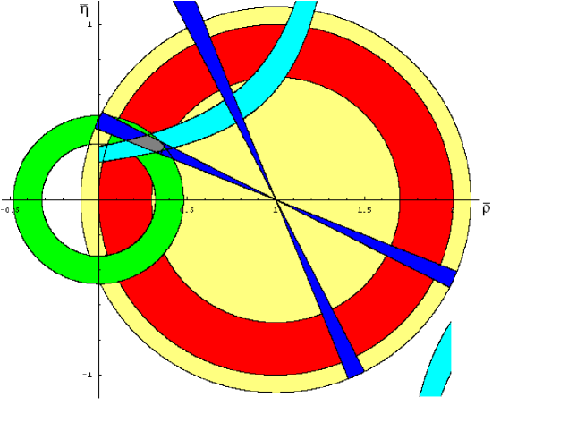
Figure 1: The domains at $(\bar{\rho},\bar{\eta})$ plane allowed at $1\sigma$ from $V_{ub}$, $\Delta m_{B_{d}}$, $\varepsilon_{K}$ and $\sin 2\beta$ measurements. 95%C.L. upper bound from the search of $\Delta m_{B_{s}}$ is shown as well.

4 Conclusions

Numerical difference of the quantities $\epsilon$ and $\tilde{\epsilon}$ (which describe $CP$-violation in $K$-mesons) was estimated in the Standard Model. Fit of CKM matrix patameters accounted for this difference was performed.

Appendix A Basic formulas for $K^{0}$-$\bar{K}^{0}$ system

It is known that states $K^{0}$ and $\bar{K}^{0}$ are not mass eigenstates. Mass eigenstates are their linear combinations:

$$K_{+}=\frac{1}{\sqrt{1+\mid\tilde{\varepsilon}\mid^{2}}}\left[\frac{K^{0}+\bar{K}^{0}}{\sqrt{2}}+\tilde{\varepsilon}\frac{K^{0}-\bar{K}^{0}}{\sqrt{2}}\right],$$ (28)

$$K_{-}=\frac{1}{\sqrt{1+\mid\tilde{\varepsilon}\mid^{2}}}\left[\frac{K^{0}-\bar{K}^{0}}{\sqrt{2}}+\tilde{\varepsilon}\frac{K^{0}+\bar{K}^{0}}{\sqrt{2}}\right].$$

Let’s denote matrix elements of the effective Hamiltonian between $K^{0}$ and $\bar{K}^{0}$ states as follows:

$$<K^{0}\mid H\mid K^{0}>=<\bar{K}^{0}\mid H\mid\bar{K}^{0}>=M-\frac{i}{2}\Gamma,$$

$$<K^{0}\mid H\mid\bar{K}^{0}>=M_{12}-\frac{i}{2}\Gamma_{12},$$

$$<\bar{K}^{0}\mid H\mid K^{0}>=M_{12}^{*}-\frac{i}{2}\Gamma_{12}^{*}.$$ (29)

The eigenvalues and eigenvectors of this matrix Hamiltonian are:

$$\lambda_{\pm}=M-\frac{i}{2}\Gamma\pm\sqrt{(M_{12}-\frac{i}{2}\Gamma_{12})(M_{12}^{*}-\frac{i}{2}\Gamma_{12}^{*})},$$

$$\left\{\begin{array}[]{l}M_{+}=pM^{0}+q\bar{M}^{0}\\ M_{-}=pM^{0}-q\bar{M}^{0}\end{array}\right.\;\;,\;\;\frac{q}{p}=\sqrt{\frac{M_{12}^{*}-\frac{i}{2}\Gamma_{12}^{*}}{M_{12}-\frac{i}{2}\Gamma_{12}}}.$$ (32)

Introducing quantity $\tilde{\varepsilon}$ according to the following definition:

$$\frac{q}{p}=\frac{1-\tilde{\varepsilon}}{1+\tilde{\varepsilon}},$$ (33)

we come to Eq.(28).

Taking into account that $\Gamma_{12}$ is real and $\displaystyle{\frac{ImM_{12}}{ReM_{12}}}\sim 0.1$ [13] we get the following expression:

$$\frac{q}{p}\approx 1-\frac{iImM_{12}}{M_{12}-\frac{i}{2}\Gamma_{12}}.$$ (34)

Eigenvalues of Hamiltonian may be written as $\lambda_{\pm}=(m_{\pm}-\frac{i}{2}\Gamma_{\pm})^{2}$, where $m_{\pm}$ are masses of corresponding states and $\Gamma_{\pm}$ - their widths. Then denoting $K_{+}$ and $K_{-}$ states as $K_{S}$ and $K_{L}$ respectively, we have $\lambda_{-}-\lambda_{+}=2m_{K}(m_{L}-m_{S}-\frac{i}{2}(\Gamma_{L}-\Gamma_{S}))$. On the other hand $\lambda_{-}-\lambda_{+}=-2\sqrt{(M_{12}-\frac{i}{2}\Gamma_{12})(M_{12}^{*}-\frac{i}{2}\Gamma_{12}^{*})}\sim-2(M_{12}-\frac{i}{2}\Gamma_{12}).$ This leads to:

$$\frac{q}{p}\approx 1+\frac{iImM_{12}/m_{K}}{(m_{L}-m_{S}-\frac{i}{2}(\Gamma_{L}-\Gamma_{S}))}\approx 1-2\tilde{\epsilon}.$$ (35)

Taking into account that $\Gamma_{S}<<\Gamma_{L}$ and $\Delta m_{LS}\approx\Gamma_{S}/2$, we obtain:

$$\tilde{\epsilon}\approx-\frac{iImM_{12}/2m_{K}}{(\Delta m_{LS}-\frac{i}{2}(\Gamma_{L}-\Gamma_{S}))}\approx e^{-i\frac{3\pi}{4}}\frac{ImM_{12}/2m_{K}}{\sqrt{2}\Delta m_{LS}}.$$ (36)

Thus calculating $ImM_{12}$ within the SM we find the theoretical prediction for $\tilde{\epsilon}$. (Let us note that since $ImM_{12}$ is negative, the phase of $\tilde{\epsilon}$ approximately equals $\frac{\pi}{4}$).

Now we proceed to decays of kaons into pairs of pions, whose amplitudes are well measured experimentally.

It is convenient to deal with the amplitudes of the decays into the states with definite isospin:

$$A(K^{0}\to\pi^{+}\pi^{-})=\frac{a_{2}}{\sqrt{3}}e^{i\xi_{2}}e^{i\delta_{2}}+\frac{a_{0}}{\sqrt{3}}\sqrt{2}e^{i\xi_{0}}e^{i\delta_{0}}$$

$$A(\bar{K}^{0}\to\pi^{+}\pi^{-})=\frac{a_{2}}{\sqrt{3}}e^{-i\xi_{2}}e^{i\delta_{2}}+\frac{a_{0}}{\sqrt{3}}\sqrt{2}e^{-i\xi_{0}}e^{i\delta_{0}}$$

$$A(K^{0}\to\pi^{0}\pi^{0})=\sqrt{\frac{2}{3}}a_{2}e^{i\xi_{2}}e^{i\delta_{2}}-\frac{a_{0}}{\sqrt{3}}e^{i\xi_{0}}e^{i\delta_{0}}$$

$$A(\bar{K}^{0}\to\pi^{0}\pi^{0})=\sqrt{\frac{2}{3}}a_{2}e^{-i\xi_{2}}e^{i\delta_{2}}-\frac{a_{0}}{\sqrt{3}}e^{-i\xi_{0}}e^{i\delta_{0}}$$ (37)

where “2” and “0” are the values of ($\pi\pi$) isospin, $\xi_{2,0}$ are the (small) weak phases which originate from CKM matrix and $\delta_{2,0}$ are the strong phases of $\pi\pi$-rescattering.

Experimentally measured quantities are:

$$\eta_{+-}=\frac{A(K_{L}\to\pi^{+}\pi^{-})}{A(K_{S}\to\pi^{+}\pi^{-})},$$

$$\eta_{00}=\frac{A(K_{L}\to\pi^{0}\pi^{0})}{A(K_{S}\to\pi^{0}\pi^{0})}.$$ (38)

For the amplitudes of $K_{L}$ and $K_{S}$ decays into $\pi^{+}\pi^{-}$ we obtain:

$$A(K_{L}\to\pi^{+}\pi^{-})=\frac{1}{\sqrt{2}}\left[\frac{a_{2}}{\sqrt{3}}e^{i\delta_{2}}2i\sin\xi_{2}+\frac{a_{0}}{\sqrt{3}}\sqrt{2}e^{i\delta_{0}}2i\sin\xi_{0}\right]+$$

$$+\frac{\tilde{\epsilon}}{\sqrt{2}}\left[\frac{a_{2}}{\sqrt{3}}e^{i\delta_{2}}2\cos\xi_{2}+\frac{a_{0}}{\sqrt{3}}\sqrt{2}e^{i\delta_{0}}2\cos\xi_{0}\right],$$

$$A(K_{S}\to\pi^{+}\pi^{-})=\frac{1}{\sqrt{2}}\left[\frac{a_{2}}{\sqrt{3}}e^{i\delta_{2}}2\cos\xi_{2}+\frac{a_{0}}{\sqrt{3}}\sqrt{2}e^{i\delta_{0}}2\cos\xi_{0}\right],$$ (39)

where in the last equation we omit the terms which are proportional to the product of two small factors, $\tilde{\epsilon}$ and $\sin\xi_{0,2}$. For the ratio of these amplitudes we get:

$$\eta_{+-}=\frac{A(K_{L}\to\pi^{+}\pi^{-})}{A(K_{S}\to\pi^{+}\pi^{-})}=\tilde{\epsilon}+i\frac{\sin\xi_{0}}{\cos\xi_{0}}+\frac{ie^{i(\delta_{2}-\delta_{0})}}{\sqrt{2}}\frac{a_{2}\cos\xi_{2}}{a_{0}\cos\xi_{0}}\left[\frac{\sin\xi_{2}}{\cos\xi_{2}}-\frac{\sin\xi_{0}}{\cos\xi_{0}}\right],$$

where we neglect the terms of the order of $(a_{2}/a_{0})^{2}\sin\xi_{0,2}$, because $a_{2}/a_{0}\approx 1/22$.

The analogous treatment of $K_{L,S}\to\pi^{0}\pi^{0}$ decay amplitudes leads to:

$$\eta_{00}=\frac{A(K_{L}\to\pi^{0}\pi^{0})}{A(K_{S}\to\pi^{0}\pi^{0})}=\tilde{\epsilon}+i\frac{\sin\xi_{0}}{\cos\xi_{0}}-ie^{i(\delta_{2}-\delta_{0})}\sqrt{2}\frac{a_{2}\cos\xi_{2}}{a_{0}\cos\xi_{0}}\left[\frac{\sin\xi_{2}}{\cos\xi_{2}}-\frac{\sin\xi_{0}}{\cos\xi_{0}}\right].$$

Introducing conventional quantities $\epsilon=\frac{2}{3}\eta_{+-}+\frac{1}{3}\eta_{00}$ and $\epsilon^{\prime}=\frac{1}{3}\eta_{+-}-\frac{1}{3}\eta_{00}$, we get:

$$\epsilon^{\prime}=\frac{i}{\sqrt{2}}e^{i(\delta_{2}-\delta_{0})}\frac{1}{ReA_{0}}\left[ImA_{2}-wImA_{0}\right]$$

$$\epsilon=\tilde{\epsilon}+i\frac{ImA_{0}}{ReA_{0}},$$ (40)

where $A_{2,0}\equiv e^{i\xi_{2,0}}a_{2,0}$, and $\displaystyle{w=\frac{ReA_{2}}{ReA_{0}}\approx\frac{a_{2}}{a_{0}}}$.

Equations (A) are our starting point in the present paper; see Introduction.