Neutrino Masses, Mixing and New Physics Effects

Abstract

We introduce a parametrization of the effects of radiative corrections from new physics on the charged lepton and neutrino mass matrices, studying how several relevant quantities describing the pattern of neutrino masses and mixing are affected by these corrections. We find that the ratio $\omega\equiv\sin\theta/\tan\theta_{\mathrm{atm}}$ is remarkably stable, even when relatively large corrections are added to the original mass matrices. It is also found that if the lightest neutrino has a mass around 0.3 eV, the pattern of masses and mixings is considerably more stable under perturbations than for a lighter or heavier spectrum. We explore the consequences of perturbations on some flavor relations given in the literature. In addition, for a quasi-degenerate neutrino spectrum it is shown that: (i) starting from a bi-maximal mixing scenario, the corrections to the mass matrices keep $\tan\theta_{\mathrm{atm}}$ very close to unity while they can lower $\tan\theta_{\odot}$ to its measured value; (ii) beginning from a scenario with a vanishing Dirac phase, corrections can induce a Dirac phase large enough to yield $CP$ violation observable in neutrino oscillations.

I Introduction

Our present knowledge of neutrino masses and mixing is mainly provided by various neutrino oscillation experiments, which give us information on the two independent mass squared differences, as well as on the three angles characterizing the leptonic mixing matrix. In the future, the study of $CP$ violation in neutrino oscillations may allow to determine the Dirac-type phase entering in the leptonic mixing matrix, and neutrinoless double $\beta$ decay experiments may provide the value of the effective Majorana mass. Despite the great achievements of oscillation experiments, there is still much to be learned about neutrinos. One of the most problematic issues in neutrino physics is the lack of information on the mass spectrum, since the mass squared differences do not fix the absolute scale of neutrino masses. Indeed, the spectrum can exhibit a strong hierarchy, as in the case of quarks and charged leptons, or on the contrary, be quasi-degenerate.

At present, there are different extensions of the standard model (SM) which propose mechanisms for the generation of neutrino masses through the enlargement of the SM particle content. The addition of heavy right-handed neutrino singlets constitutes a simple and economical way to give left-handed neutrinos small masses through the seesaw mechanism seesaw1 ; seesaw2 ; seesaw3 ; seesaw4 . Another simple possibility relies on the extension of the scalar sector with a heavy $\mathrm{SU}(2)_{L}$ triplet, with or without supersymmetry (SUSY) Cheng:qt ; Gelmini:1980re ; Wetterich:1981bx ; Rossi:2002zb . Within supersymmetric models, neutrino masses can also arise from $R$-parity violating interactions Diaz:2003as , where the atmospheric and solar neutrino mass scales are generated at the tree level and radiatively, respectively. Recently, a new supersymmetric source of neutrino masses and mixings has been found considering non-renormalizable lepton number violating interactions in the Kähler potential Casas:2002sn rather than in the effective superpotential. All the above scenarios predict the existence of light Majorana massive neutrinos. Suppressed Dirac neutrino masses are unnatural in conventional theories since they usually require extremely small Yukawa couplings. However, this problem can be surmounted by endowing the particle content of the theory with extra fermion or scalar fields and/or introducing new symmetries dirac1 ; dirac1b ; dirac2 ; dirac3 ; dirac4 . Naturally small Dirac neutrino masses also arise in extra-dimensional theories as a consequence of the small overlap between the wavefunctions of the usual left-handed neutrinos in the brane and the sterile right-handed ones in the bulk (or in other branes) extra1 ; extra2 ; extra3 ; barenboim ; extra4 ; extra5 .

In addition to the mechanism for the generation of neutrino masses, one of the most intriguing aspects of leptonic physics is the experimental evidence that two of the lepton mixing angles are large, in contrast to the small mixing observed in the quark sector. The deep understanding of the neutrino mass suppression mechanism and the bi-large leptonic mixing constitutes one of the most challenging questions in particle physics. A theory of leptonic flavor should provide a plausible explanation for the bi-large mixing, as well as for the neutrino mass spectrum. At the same time, it should predict relations among these quantities. There have been in the literature a large number of suggestions in this direction, consisting in the introduction of flavor symmetries or the assumption of specific textures for the leptonic mass matrices models ; reviews .

The tree-level predictions of any theory of leptonic flavor are subject to higher order corrections, which are computable if the particle content and parameters of the new physics model are specified. Still, in the absence of a “standard theory” of lepton flavor, it is pertinent to ask ourselves about the possible consequences of the (unknown) radiative corrections on the tree-level predictions of the model. The aim of this paper is to investigate these effects, focusing on: (i) the modification of the tree-level values for the ratio of mass squared differences, mixing angles and CP violation parameters; (ii) the effect on various flavor relations. This task will be carried out in two steps. We will first propose a parametrization for the unknown radiative corrections to the lepton mass matrices, based on rather general arguments on weak-basis independence. In this parametrization, the formal structure of the corrections is fixed, up to undetermined complex coefficients. Then, the possible effects of the radiative corrections is investigated taking these coefficients as random, and performing a statistical analysis of the average behavior of the parameters and flavor relations under consideration.

It is important to note here the difference between our framework and other studies in the literature regarding random neutrino matrices murayama ; vissani ; masina ; espinosa . In these analyses, the neutrino mass matrices are taken as random at the tree level, with a subsequent discussion of the predictions for the neutrino mass spectrum and mixing angles. In contrast with this approach, in this paper we take the tree-level charged lepton and neutrino mass matrices as fixed by some theory of leptonic flavor, and consider random perturbations (from radiative corrections) to them anarch . These corrections are not completely arbitrary: the different terms of the perturbations must have a determined formal structure (which is dictated by weak basis independence) but have random coefficients.

This paper is organized as follows. In Section II we briefly review the current status of neutrino oscillation data. The parametrization of the unknown corrections to the lepton mass matrices is derived in Section III. In Section IV we present our results, discussing (i) the effect of perturbations on masses and mixing parameters; (ii) the influence on some flavor relations obtained for some specific patterns in the literature; (iii) the consequences of the corrections in some special limits of interest. Our conclusions are summarized in Section V.

II Neutrino oscillations: present status

All presently available neutrino oscillation data can be accommodated within the framework of three mixed massive neutrinos Giunti:2003qt . The first KamLAND results Eguchi:2002dm select the large mixing angle MSW solution as the only surviving explanation for the solar neutrino problem. In addition, dominant solar neutrino conversion based on non-oscillation solutions are now excluded valle1 ; valle2 . Recently, the Sudbury Neutrino Observatory (SNO) has released the improved measurements of the salt enhanced phase Ahmed:2003kj which, together with all the solar and KamLAND neutrino data, allow for a better determination of the oscillation parameters. In particular, the high-$\Delta m^{2}$ region ($\Delta m_{\odot}^{2}>10^{-4}\,{\rm eV^{2}}$) is now only accepted at the $3\sigma$ level and maximal solar mixing is ruled out by more than $5\sigma$, rejecting in this way the possibility of bi-maximal leptonic mixing Balantekin ; fogli ; maltoni ; aliani ; petcov ; creminelli ; deHolanda:2003nj . Concerning the atmospheric neutrino sector, the water Cherenkov Super-Kamiokande (SK) Fukuda:1998mi and long-baseline KEK-to-Kamioka (K2K) Ahn:2002up experiments indicate that neutrino flavor conversion due to neutrino oscillations in the $\nu_{\mu}\rightarrow\nu_{\tau}$ channel provide by far the most acceptable and natural explanation for the observed $\nu_{\mu}$ disappearance.

Regarding the absolute values of neutrino masses, the situation is not so satisfactory. At present, the most stringent direct bound on the neutrino mass is provided by the Mainz Bonn:jw and Troitsk Lobashev:uu experiments, which have set a maximum value for $m_{\nu_{e}}$ of $2.2\,{\rm eV}$. Neutrinoless double beta-decay measurements may also be valuable to disentangle the pattern of neutrino masses, although in this case certain subtleties have to be considered Joaquim:2003pn .

Throughout this paper we adopt the neutrino mass ordering $m_{1}<m_{2}<m_{3}$ in such a way that, for the hierarchical (HI), inverted-hierarchical (IH) and quasi-degenerate (QD) neutrino mass spectra one has

HI $$\rightarrow m_{1}\ll m_{2}\,,\,m_{3}\,,~{}\Delta m_{\odot}^{2}=\Delta m^{2}_{21}\,;$$

IH $$\rightarrow m_{1}\ll m_{2}\,,\,m_{3}\,,~{}\Delta m_{\odot}^{2}=\Delta m^{2}_{32}\,;$$

QD $$\rightarrow m_{1}\simeq m_{2}\simeq m_{3}\,,~{}\Delta m_{\odot}^{2}=\Delta m^{2}_{21}\,,\,$$ (1)

where $\Delta m_{\odot}^{2}$ and $\Delta m_{\rm atm}^{2}=\Delta m^{2}_{31}\gg\Delta m_{\odot}^{2}$ are the solar and atmospheric neutrino mass squared differences, respectively. At the $1\sigma$ level, the allowed ranges for $\Delta m_{\odot}^{2}$ and $\Delta m_{\rm atm}^{2}$ are deHolanda:2003nj ; Fogli:2003th

$$\Delta m_{\odot}^{2}=(6.5-8.5)\times 10^{-5}\,{\rm eV}^{2}\,,$$

$$\Delta m_{\rm atm}^{2}=(2.6\pm 0.4)\times 10^{-3}\,{\rm eV}^{2}\,,$$ (2)

with the best-fit values

$$\Delta m_{\odot}^{2}=7.13\times 10^{-5}\,{\rm eV}^{2}\,,$$

$$\Delta m_{\rm atm}^{2}=2.6\times 10^{-3}\,{\rm eV}^{2}\,.$$ (3)

For three light Majorana neutrinos, the leptonic mixing matrix $U$ can be written as

$$U=\left(\begin{array}[]{ccc}U_{e1}&U_{e2}&U_{e3}\\ U_{\mu 1}&U_{\mu 2}&U_{\mu 3}\\ U_{\tau 1}&U_{\tau 2}&U_{\tau 3}\end{array}\right)=U_{\delta}\,\text{diag}(e^{-i\alpha},e^{-i\beta},1)\,,$$ (7)

where $\alpha$ and $\beta$ are Majorana-type phases and $U_{\delta}$ can be parametrized in the form

$$U_{\delta}=\left(\begin{array}[]{ccc}c_{3}c_{2}&s_{3}c_{2}&s_{2}e^{-i\delta}\\ -s_{3}c_{1}-c_{3}s_{1}s_{2}e^{i\delta}&c_{3}c_{1}-s_{3}s_{1}s_{2}e^{i\delta}&s_{1}c_{2}\\ s_{3}s_{1}-c_{3}c_{1}s_{2}e^{i\delta}&-c_{3}s_{1}-s_{3}c_{1}s_{2}e^{i\delta}&c_{1}c_{2}\end{array}\right)$$ (11)

with $s_{i}\equiv\sin\theta_{i}$, $c_{i}\equiv\cos\theta_{i}$ $(i=1,2,3)$ and $\delta$ the Dirac-type $CP$-violating phase. For Dirac neutrinos $U$ reduces to $U_{\delta}$, due to the absence of Majorana phases. Depending on the type of neutrino mass spectrum, the solar, atmospheric and CHOOZ Apollonio:1999ae mixing angles ($\theta_{\odot}$, $\theta_{\rm atm}$ and $\theta$, respectively) can be extracted from $U$ in the following way: for the HI and QD neutrino mass spectra,

$$\tan\theta_{\odot}=\frac{|U_{e2}|}{|U_{e1}|}=\tan\theta_{3}\,\,,\,\,\tan\theta_{\rm atm}=\frac{|U_{\mu 3}|}{|U_{\tau 3}|}=\tan\theta_{1}\,,$$

$$\sin\theta=|U_{e3}|=\sin\theta_{2}\,,$$ (12)

and for an IH spectrum,

$$\tan\theta_{\odot}=\frac{|U_{e3}|}{|U_{e2}|}\,\,,\,\,\tan\theta_{\rm atm}=\frac{|U_{\mu 1}|}{|U_{\tau 1}|}\,\,,\,\,\sin\theta=|U_{e1}|\,.$$ (13)

In this case the expression of $\theta_{\odot}$, $\theta_{\mathrm{atm}}$ and $\theta$ in terms of $\theta_{1-3}$ in the parametrization of Eq. (11) is not simple. From the global analyses performed in Refs. deHolanda:2003nj and Fogli:2003th , the solar and atmospheric mixing angles are constrained to lay in the $1\sigma$ intervals

$$\tan^{2}\theta_{\odot}=(0.33-0.47)\,\,,\,\,\sin^{2}2\theta_{\rm atm}=1.00^{+0.00}_{-0.05}\,,$$ (14)

with the best-fit values

$$\tan^{2}\theta_{\odot}=0.39\,\,,\,\,\sin^{2}2\theta_{\rm atm}=1.00\,.$$ (15)

For $\sin\theta$ we quote the result from combined analysis of the solar neutrino, CHOOZ and KamLAND data performed in Ref. Fogli:2002au ,

$$\sin\theta<0.18\,,$$ (16)

with a 95% confidence level (CL).

The upcoming long-baseline neutrino oscillation experiments will face the challenge of detecting $CP$-violating effects induced by the Dirac phase $\delta$ Lindner:2002vt . The difference of the $CP$-conjugated neutrino oscillation probabilities $P(\nu_{e}\rightarrow\nu_{\mu})-P(\bar{\nu}_{e}\rightarrow\bar{\nu}_{\mu})$ is proportional to the quantity

$${\cal J} \equiv{\rm Im}\left[\,U_{e1}U_{\mu 2}U_{e2}^{\ast}U_{\mu 1}^{\ast}\,\right]$$

$$=\frac{1}{8}\sin 2\theta_{1}\;\sin 2\theta_{2}\;\sin 2\theta_{3}\;\sin\delta\,.$$ (17)

Present estimates indicate that for $|\mathcal{J}|\gtrsim 10^{-2}$ it will be possible to observe $CP$ violation effects in these experiments.

III Parametrizing the new physics contributions to lepton masses

Before electroweak symmetry breaking (EWSB), the terms of the Lagrangian that originate the charged lepton and light Majorana neutrino masses can be written as

$$\mathcal{L}=-Y^{e}_{ij}\,\bar{\ell}_{Li}\,\phi\,e_{Rj}+\frac{A_{ij}}{\Lambda}(\bar{\ell}_{Li}\,i\sigma_{2}\,\phi^{*})\,(\phi^{\dagger}\,i\sigma_{2}\,\ell_{Lj}^{c})+\mathrm{H.c.}\,,$$ (18)

where $\ell_{Li}=(\nu_{Li}~{}e_{Li})^{T}$, $\phi=(\phi^{+}~{}\phi^{0})^{T}$ is the SM Higgs doublet and $Y^{e}$ is the usual $3\times 3$ matrix of the charged lepton Yukawa couplings. The second term is a neutrino mass operator weinberg generated by physics above the electroweak scale, being $A$ a $3\times 3$ symmetric matrix of dimensionless couplings of order unity and $\Lambda$ the scale at which this interaction is generated. These vertices can be depicted by the Feynman diagrams in Fig. 1, where the flavor dependence of each vertex is explicitly shown. The arrows in the scalar lines indicate the flow of the positive charge for the $T=1/2$ component of the doublet.

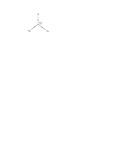
Figure 1: Feynman diagrams corresponding to the vertices in Eq. (18). In each vertex the flavor dependence is explicitly shown.

There are different mechanisms that may lead to the neutrino mass operator given in Eq. (18). In particular, it may be originated by a heavy scalar triplet $\Delta$, which is conveniently written in matrix form as

$$\Delta=\left(\begin{array}[]{cc}\Delta^{+}&\sqrt{2}\Delta^{++}\\ \sqrt{2}\Delta^{0}&-\Delta^{+}\end{array}\right)\,.$$ (19)

This scalar triplet couples to the lepton and Higgs doublets as

$$\mathcal{L}_{\Delta}=Y^{\Delta}_{ij}\,\bar{\ell}_{i}\,\Delta^{\dagger}\,i\sigma_{2}\,\ell_{j}^{c}+g_{\Delta\phi}\,\phi^{\dagger}\Delta\,i\sigma_{2}\,\phi^{*}+\mathrm{H.c.}\,,$$ (20)

where $Y^{\Delta}$ is a matrix of Yukawa couplings and $g_{\Delta\phi}$ has dimension of mass. The exchange of the heavy triplet results in an effective neutrino mass operator, given by

$$\frac{A_{ij}}{\Lambda}=Y^{\Delta}_{ij}\frac{g_{\Delta\phi}}{m_{\Delta}^{2}}\,,$$ (21)

with $m_{\Delta}$ the mass of the triplet.

Another possibility is the exchange of heavy right-handed neutrinos $\nu_{R}$ (the seesaw mechanism). In this case, the relevant terms are

$$\mathcal{L}_{\nu_{R}}=-Y^{\nu}_{ij}\,\bar{\ell}_{Li}\,i\sigma_{2}\,\phi^{*}\,\nu_{Rj}-\frac{1}{2}M_{Rij}\,\overline{\nu_{Ri}^{c}}\nu_{Rj}+\mathrm{H.c.}\,,$$ (22)

with $Y^{\nu}$ is the Dirac neutrino Yukawa coupling matrix and $M_{R}$ the heavy right-handed neutrino mass matrix. The integration of the heavy neutrino fields generates an effective mass operator for the light neutrinos of the form

$$\frac{A_{ij}}{\Lambda}=-\frac{1}{2}(Y^{\nu}M_{R}^{-1}Y^{\nu T})_{ij}\,.$$ (23)

After EWSB, the terms in Eq. (18) yield the mass terms for the charged leptons and left-handed neutrinos. Using matrix notation in flavor space, the mass terms can be written as

$$\mathcal{L}_{m}=-\bar{e}_{L}M_{e}e_{R}-\frac{1}{2}\bar{\nu}_{L}M_{L}\nu_{L}^{c}\,,$$ (24)

where $M_{e}=v\,Y^{e}$ and $M_{L}=2A\,v^{2}/\Lambda$, with $v=174$ GeV the vacuum expectation value (VEV) of the SM Higgs boson.

Our parametrization of the new physics effects is obtained after general considerations on weak basis independence. For convenience, let us define

$$\hat{M}_{L}\equiv\varepsilon\,A=\frac{\varepsilon\Lambda}{2v^{2}}\,M_{L}\equiv\frac{M_{L}}{\mathcal{N}}\,,$$ (25)

with $\varepsilon$ a dimensionless parameter to be specified later. Under the change of weak basis

$$\ell_{L}=V_{L}~{}\ell^{\prime}_{L}\,,\quad e_{R}=V_{R}^{e}~{}e^{\prime}_{R}$$ (26)

we have

$$Y^{e}\to V_{L}^{\dagger}\,Y^{e}\,V_{R}^{e}\,,\quad\hat{M}_{L}\to V_{L}^{\dagger}\hat{M}_{L}V_{L}^{*}\,.$$ (27)

Let us assume that some perturbations arising from radiative corrections are added to the “tree-level” matrices $Y^{e}$ and $\hat{M}_{L}$,

$$Y^{e}\to Y^{e}+\delta Y^{e}\,,\quad\hat{M}_{L}\to\hat{M}_{L}+\delta\hat{M}_{L}\,.$$ (28)

The matrices $\delta Y^{e}$, $\delta\hat{M}_{L}$ are functions of $Y^{e}$, $\hat{M}_{L}$ and other SM and new physics parameters. Under the change of basis defined in Eqs. (26), the perturbations must transform as

$$\delta Y^{e}\to V_{L}^{\dagger}\,\delta Y^{e}\,V_{R}^{e}\,,\quad\delta\hat{M}_{L}\to V_{L}^{\dagger}\,\delta\hat{M}_{L}\,V_{L}^{*}\,,$$ (29)

since the physical observables must be independent of the choice of weak basis. These transformation laws imply that the perturbations have the form anarch

$$\delta Y^{e} = \lambda_{e}\,Y^{e}+\zeta_{e}\,Y^{e}Y^{e\dagger}Y^{e}+\eta_{e}\,\hat{M}_{L}\hat{M}_{L}^{\dagger}Y^{e}+\cdots\,,$$

$$\delta\hat{M}_{L} = \lambda_{L}\,\hat{M}_{L}+\zeta_{L}\,\hat{M}_{L}\hat{M}_{L}^{\dagger}\hat{M}_{L}$$ (30)

$$+\eta_{L}\left(Y^{e}Y^{e\dagger}\hat{M}_{L}+\hat{M}_{L}Y^{e*}Y^{eT}\right)+\cdots\,,$$

where the $\lambda_{i}$, $\zeta_{i}$ and $\eta_{i}$ coefficients ($i=e,L$) are functions of $Y^{e}$, $\hat{M}_{L}$ and of the coupling constants, which are invariant under the transformations of Eqs. (26) and in general complex. The higher order terms in this expansion are expected to be smaller. The effect of the $\lambda_{i}$ terms in Eqs. (30) is to rescale the masses by common factors $(1+\lambda_{e})$ for charged leptons and $(1+\lambda_{L})$ for neutrinos, without affecting neither the mass hierarchy nor the mixing. The $\zeta_{i}$ terms also rescale the masses, but with a different factor for each lepton: $m_{e_{j}}\to m_{e_{j}}\,(1+\zeta_{e}\,m_{e_{j}}^{2}/v^{2})$ for charged leptons and $m_{j}\to m_{j}\,(1+\zeta_{L}\,m_{j}^{2}/\mathcal{N}^{2})$ for neutrinos. Hence, the $\zeta_{i}$ terms modify the mass hierarchies. The $\eta_{i}$ terms are the lowest-order ones which modify the leptonic mixing.

For some SM extensions, in principle there may exist a matrix $X$ (not necessarily square) of couplings between the leptons and other particles, transforming as $Y^{e}$ or $\hat{M}_{L}$ either on the left or on the right side. For instance, if $X$ transforms under the change of basis in Eqs. (26) as

$$X\to V_{L}^{\dagger}\,X\,V_{R}^{X}\,,$$ (31)

this matrix would contribute to $\delta Y^{e}$ and $\delta\hat{M}_{L}$ with terms $XX^{\dagger}Y^{e}$ and $(XX^{\dagger}\hat{M}_{L}+\hat{M}_{L}X^{*}X^{T})$, respectively. Such possibility will not be considered in the following, and in this respect our analysis is not be the most general one. We thus assume $Y^{e}$ and $\hat{M}_{L}$ as the only sources of flavor violation in the lepton sector. This case can naturally arise if some symmetry relates the couplings in Eq. (18) with the ones between the leptons and the new particles.

It is worthwhile showing some examples of Feynman diagrams which contribute to the different terms in Eqs. (30) within the SM, including also the effective neutrino mass operator in Eq. (18) as part of the SM vertices. The $\lambda_{i}$ terms result from diagrams with minimal flavor structure, as for example diagrams (a) and (b) in Fig. 2, with the exchange of a $B$ boson with flavor-universal couplings. The remaining terms in Eqs. (30) require the exchange of one or more $\phi$ doublets. In particular, the $\zeta_{e}$ and $\eta_{L}$ terms arise from diagrams like (c) and (d) in Fig. 2, respectively. At the one loop level the terms with $\eta_{e}$ and $\zeta_{L}$ are absent, and to generate them it is necessary to consider two-loop corrections, for instance diagrams (e) and (f), respectively.

(a)	(b)
(c)	(d)
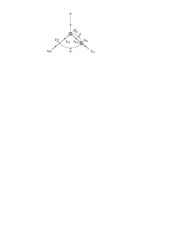
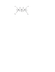
(e)	(f)

Figure 2: Examples of SM diagrams giving corrections to the $\ell_{L}\phi\,e_{R}$ and $\ell_{L}\ell_{L}^{c}\phi^{*}\phi^{*}$ vertices. In each vertex the flavor dependence is explicitly shown.

In new physics scenarios there are additional interactions that may or may not be suppressed by a large scale $\Lambda^{\prime}$. These interactions mediate Feynman diagrams giving further corrections to the $\ell_{L}\phi\,e_{R}$ and $\ell_{L}\ell_{L}^{c}\phi^{*}\phi^{*}$ vertices. Several examples of new physics contributions to these operators can be found in Ref. smirnov . We remark that, if the particle content and parameters of the new physics model are specified, the corrections to the charged lepton and neutrino mass matrices can be completely determined. However, in the absence of any experimental indication favoring any of the theories beyond the SM, the $\lambda_{i}$, $\zeta_{i}$, $\eta_{i}$ coefficients cannot be predicted. Then, it is sensible to perform a statistical analysis in order to determine, under certain assumptions, how much the tree-level predictions can change due to radiative corrections from new physics, parametrized according to Eq. (30), leaving $\lambda_{i}$, $\zeta_{i}$, $\eta_{i}$ as unknown parameters. The size of these coefficients is expected to be similar, because all the terms in Eqs. (30) can be generated at the one loop level (although the terms with $\eta_{e}$ and $\zeta_{L}$ appear at next-to-leading order within the SM, they may arise at leading order in other models, e.g. with a scalar triplet). On the other hand, the higher order terms omitted in Eqs. (30), involving products of 5 matrices or more, are expected to be suppressed by a factor $\sim 10$ with respect to the leading ones.

One crucial issue for our analysis is the value of the parameter $\varepsilon$ in Eq. (25), which accounts for the normalization of $\hat{M}_{L}$. The size of this parameter reflects the suppression of the new interactions, and determines the relative importance of $\hat{M}_{L}$ with respect to $Y^{e}$ in the expressions used for the perturbations. We consider two limiting scenarios:

(i) In the first scenario we take $\varepsilon=1$, in which case $\hat{M}_{L}=A$ with matrix elements of order unity. This corresponds to a situation where there are new interactions which are not suppressed by a large scale $\Lambda^{\prime}$. In this scenario, the terms $\zeta_{L}\,\hat{M}_{L}\hat{M}_{L}^{\dagger}\hat{M}_{L}$ and $\eta_{e}\,\hat{M}_{L}\hat{M}_{L}^{\dagger}Y^{e}$ in Eqs. (30) are not negligible, and have an important influence on the neutrino mass hierarchy and mixing, respectively.

(ii) In the second scenario we assume $\varepsilon\ll 1$, so that these two terms (which have two or more powers of $\hat{M}_{L}$) can be omitted in Eqs. (30), resulting in

$$\delta Y^{e}|_{\mathrm{S2}} = \lambda_{e}\,Y^{e}+\zeta_{e}\,Y^{e}Y^{e\dagger}Y^{e}+\cdots\,,$$

$$\delta\hat{M}_{L}|_{\mathrm{S2}} = \lambda_{L}\,\hat{M}_{L}+\eta_{L}\left(Y^{e}Y^{e\dagger}\hat{M}_{L}+\hat{M}_{L}Y^{e*}Y^{eT}\right)$$ (32)

$$+\cdots\,.$$

This scenario corresponds to a new physics model in which the new interactions are suppressed by a large scale $\Lambda^{\prime}\sim\Lambda$, for instance in models based in the seesaw mechanism. In the limit $\varepsilon\ll 1$, the normalization of $\hat{M}_{L}$ is irrelevant.

From Eqs. (32) we see that in scenario 2 the expressions for the perturbations are formally similar to the one loop RG equations within the SM. Therefore, in this scenario the results obtained within our framework are expected to be similar to the results of RG evolution, bearing in mind that in the case of the RG equations the coefficients $\lambda_{i}$, $\zeta_{e}$ and $\eta_{L}$ are fixed, while in our case they are unknown in principle.

If the neutrinos are not Majorana but Dirac particles, the Yukawa term of the Lagrangian originating their masses reads

$$\mathcal{L}_{D}=-Y^{\nu}_{ij}\,\bar{\ell}_{Li}\,i\sigma_{2}\phi^{*}\,\nu_{Rj}+\mathrm{H.c.}$$ (33)

For this term and the charged lepton one, the change of basis analogous to Eqs. (26) reads

$$\ell_{L}=V_{L}~{}\ell^{\prime}_{L}\,,\quad e_{R}=V_{R}^{e}~{}e^{\prime}_{R}\,,\quad\nu_{R}=V_{R}^{\nu}~{}\nu^{\prime}_{R}\,.$$ (34)

Under this transformation, the Yukawa matrices transform as

$$Y^{e}\to V_{L}^{\dagger}\,Y^{e}\,V_{R}^{e}\,,\quad Y^{\nu}\to V_{L}^{\dagger}\,Y^{\nu}\,V_{R}^{\nu}\,.$$ (35)

This allows to obtain the expressions for the perturbations for Dirac neutrinos,

$$\delta Y^{e} = \lambda_{e}\,Y^{e}+\zeta_{e}\,Y^{e}Y^{e\dagger}Y^{e}+\eta_{e}\,Y^{\nu}\hat{Y}^{\nu\dagger}Y^{e}+\cdots\,,$$

$$\delta Y^{\nu} = \lambda_{\nu}\,Y^{\nu}+\zeta_{\nu}\,Y^{\nu}Y^{\nu\dagger}Y^{\nu}+\eta_{\nu}\,Y^{e}Y^{e\dagger}Y^{\nu}$$ (36)

$$+\cdots\,.$$

In the following, we will generally refer to the case where neutrinos are Majorana particles, and quote the results for Dirac neutrinos when relevant.

IV Numerical results

Using the parametrization of new physics contributions given in Eqs. (30), (32), (36), we study the changes in the pattern of neutrino masses and mixings due to these corrections. For this purpose, we take the unknown coefficients $\lambda_{i}$, $\zeta_{i}$, $\eta_{i}$ as random complex parameters, generated with a Gaussian distribution centered at zero and, for simplicity, we assume that the standard deviations coincide:

$$\langle|\lambda_{i}|^{2}\rangle^{\frac{1}{2}}=\langle|\zeta_{i}|^{2}\rangle^{\frac{1}{2}}=\langle|\eta_{i}|^{2}\rangle^{\frac{1}{2}}\equiv\kappa\,.$$ (37)

Contrarily to what could be expected, this is not a serious bias in the analysis, because the moduli of the random parameters are not constrained to be all equal, and only the standard deviations of the distributions are assumed to be the same. The phases of $\lambda_{i}$, $\zeta_{i}$ and $\eta_{i}$ are generated uniformly between $0$ and $2\pi$. In our study the following procedure is applied: we fix a value of $\kappa$ and generate a large set of matrices using Eqs. (30), (32) or (36), as appropriate, with random coefficients $\lambda_{i}$, $\zeta_{i}$, $\eta_{i}$. These matrices are diagonalized in order to obtain the masses and the neutrino mixing matrix. We then select some observable, and examine its distribution over the set of matrices. For each value of $\kappa$, the $1\sigma$ limits on this observable are defined as the boundaries of the 68.3% confidence level central interval, evaluated from the sample of random matrices. These $1\sigma$ limits reflect the “average” behavior of the observable under consideration, when arbitrary perturbations are added to the original matrices. It must be emphasized that the maximum and minimum values can be very different from the average values, and some situations are found where in average the observable does not change appreciably under perturbations, but for fine-tuned values of the random parameters it does.

In the numerical analysis we take initial “tree-level” matrices $Y^{e}$ and $\hat{M}_{L}$ ($Y^{\nu}$ for Dirac neutrinos) reproducing the current experimental data summarized in Section II. The charged lepton masses are taken at the scale $M_{Z}$ koide . We assume $\sin\theta=0.15$ and fix the Dirac and Majorana phases to be $\delta=\pi/2$, $\alpha=\pi/3$ and $\beta=\pi/5$. We analyze separately the two possibilities of a HI or a QD spectrum. For the case of an inverted hierarchy the results turn out to be very similar to those found for a normal hierarchy, and we do not present them. We summarize our input values in Table 1. In scenario 1, we take $\hat{M}_{L}$ with the mass of the heaviest neutrino normalized to unity. The normalization of $\hat{M}_{L}$ is irrelevant in scenario 2, as shown in the previous section.

Parameter	Value
$m_{e}$	$0.487$ MeV
$m_{\mu}$	0.103 GeV
$m_{\tau}$	1.747 GeV
$m_{1}$	$\left\{\mbox{\begin{tabular}[]{l}$10^{-5}$ eV (HI)\\ 1 eV (QD)\end{tabular}}\right.$
$\Delta m_{\odot}^{2}$	$7.13\times 10^{-5}$ eV
$\Delta m_{\mathrm{atm}}^{2}$	$2.6\times 10^{-3}$ eV
$\tan\theta_{\odot}$	0.62
$\tan\theta_{\mathrm{atm}}$	1
$\sin\theta$	0.15
$\delta$	$\pi/2$
$\alpha$	$\pi/3$
$\beta$	$\pi/5$

Table 1: Input parameters used for the unperturbed mass matrices.

IV.1 Stability of mass and mixing parameters

Let us discuss how the parameters $r\equiv\Delta m^{2}_{\odot}/\Delta m^{2}_{\mathrm{atm}}$, $\tan\theta_{\odot}$, $\tan\theta_{\mathrm{atm}}$ and $\sin\theta$ change when corrections are added to the mass matrices. Our aim is to investigate whether these quantities are stable or not, and to what extent they get modified by the perturbations. We first present the results for scenario 1, and later discuss the differences with scenario 2 and the results for Dirac neutrinos.

Regarding the ratio of mass squared differences $r$, we observe in Fig. 3 that the corrections to the matrices have a large impact on this quantity, both in the cases of a HI or QD spectrum. This plot (and the remaining ones in this section) must be interpreted with caution: it does not provide any limit on the size of the corrections, on the basis of the experimental measurement of $r$, because the initial “tree-level” value we use for $r$ needs not be equal to the observed value. Instead, the meaning of the plot is that $r$ is not stable under perturbations, and from an initial value chosen to be $r=0.027$ one can obtain values between 0.021 and 0.034, for a HI spectrum and $\kappa=0.2$.

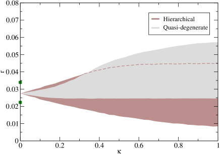
Figure 3: Effect of the perturbations on the ratio $r$ in scenario 1. For illustration, the present $1\sigma$ limits are displayed on the vertical axis.

The effect of the perturbations on $\tan\theta_{\odot}$ is quite different for a HI or QD spectrum. In the former case, $\tan\theta_{\odot}$ is very stable even for relatively large perturbations, as can be noticed in Fig. 4. On the contrary, for quasi-degenerate neutrinos, the value of $\tan\theta_{\odot}$ can change significantly with new physics corrections. This fact suggests that, if neutrinos are quasi-degenerate, the underlying tree-level pattern of lepton mass matrices could correspond to bi-maximal mixing, being the observed value $\tan\theta_{\odot}\simeq 0.6$ the result of radiative corrections. We will analyze in detail this possibility at the end of this section.

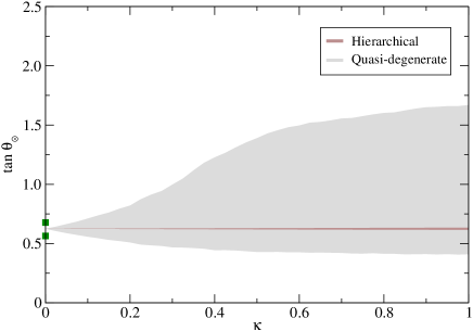
Figure 4: Effect of the perturbations on $\tan\theta_{\odot}$ in scenario 1. For illustration, the present $1\sigma$ limits are displayed on the vertical axis.

The behavior of $\tan\theta_{\mathrm{atm}}$ is the opposite to the one observed for $\tan\theta_{\odot}$, as it can be perceived from Fig. 5: for a HI spectrum this parameter is modified by perturbations on the mass matrices, while for a QD spectrum it is fairly stable. This shows that, for the case of quasi-degenerate neutrinos, the experimental observation of $\tan\theta_{\mathrm{atm}}\simeq 1$ must correspond to $\tan\theta_{\mathrm{atm}}\simeq 1$ in the mass matrices, because this prediction is not altered by the corrections. On the other hand, for a HI spectrum the observation of $\tan\theta_{\mathrm{atm}}\simeq 1$ could be either a coincidence, or result from a specific symmetry leading naturally to this value and making higher order corrections very small.

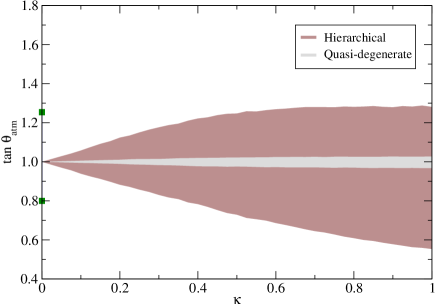
Figure 5: Effect of the perturbations on $\tan\theta_{\mathrm{atm}}$ in scenario 1. For illustration, the present $1\sigma$ limits are displayed on the vertical axis.

The analysis of $\sin\theta$ (which equals $|U_{e3}|$ for a normal hierarchy) shows that it does not change under perturbations for a QD spectrum, but it is considerably modified when the neutrino masses are hierarchical (see Fig. 6). However, one striking feature of our analysis is that the ratio

$$\omega=\frac{\sin\theta}{\tan\theta_{\mathrm{atm}}}$$ (38)

remains practically constant even when large perturbations are added to $Y^{e}$ and $\hat{M}_{L}$: for $\kappa=1$ $\sin\theta$ and $\tan\theta_{\mathrm{atm}}$ change by more than $\pm 40$%, while their ratio changes less than 1%, as can be noticed in Fig. 7.

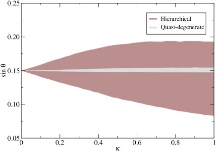
Figure 6: Effect of the perturbations on $\sin\theta$ in scenario 1.

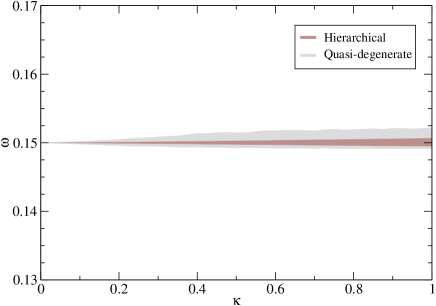
Figure 7: Effect of the perturbations on the ratio $\omega=\sin\theta/\tan\theta_{\mathrm{atm}}$ in scenario 1.

This feature may have important consequences for model building. When $\sin\theta$ is experimentally measured, the ratio $\omega$ will be an excellent tool to investigate the structure of the lepton mass matrices, because it is very insensitive to radiative corrections (as long as these corrections do not have any additional source of flavor violation, which is the framework we consider). This ratio will then allow to test experimentally, with a “clean” observable, the textures for lepton mass matrices implied by flavor symmetries proposed in the literature.

The remaining parameters to be investigated are the $CP$ violating phases, for which the results depend on the initial values used (see Table 1). For a HI spectrum, the Dirac phase $\delta$ remains virtually constant at its initial value, while the Majorana phases $\alpha$ and $\beta$ vary over a wide range, $0.6\leq\alpha\leq 2$, $0.4\leq\beta\leq 2.2$ for $\kappa=1$. For a QD spectrum, the Majorana phases remain within $\pm 10$% of their initial value for $\kappa=1$, while the Dirac phase varies in the interval $1\leq\delta\leq 1.8$.

In scenario 2, the behavior is very different for a HI spectrum. In this case, we find that $r$, $\tan\theta_{\odot}$, $\tan\theta_{\mathrm{atm}}$, $\sin\theta$ and the three $CP$ violating phases remain constant when the perturbations in Eqs. (32) are added to the matrices. In the SM these quantities exhibit a similar behavior under RG evolution RGevol , as its expressions are formally identical to ours. On the other hand, in the case of a QD spectrum, the differences between scenarios 1 and 2 are not significant, and the discussion above applies also to scenario 2. This contrast can be understood in view of the analysis of the dependence on the neutrino masses presented in Section IV.2 below.

For Dirac neutrinos, the results are found to be rather similar to the ones obtained in scenario 2. For a HI spectrum the parameters under consideration do not change when the perturbations in Eqs. (36) are included. For a QD spectrum, however, they are modified, following practically the same behavior that can be observed in the plots for scenario 1 shown in this section.

Finally, we note that the results on $r$, $\tan\theta_{\odot}$ and $\tan\theta_{\mathrm{atm}}$ are almost independent on the value of $\sin\theta$ used. Other quantities obviously depend on the particular value of $\sin\theta$, as for example $\mathcal{J}$, which is proportional to $\sin\theta$. The choice of the $CP$-violating phases is only relevant for the “tree-level” values of quantities that depend on them, like $\mathcal{J}$ and $m_{ee}$. For a QD spectrum, the deviations of $r$, $\tan\theta_{\odot}$, $\tan\theta_{\mathrm{atm}}$, $\sin\theta$ and $\omega$ are very similar, and for a HI spectrum the influence of phases on these quantities is completely negligible. We have also checked that our results do not change when the next terms in the expansion of Eqs. (30) (with products of 5 matrices) are included, even in the unrealistic limit where these terms have similar coefficients. We have found that the quantities that are stable remain stable, and the quantities that change under perturbations exhibit an analogous behavior with the inclusion of these terms.

IV.2 Dependence on the neutrino masses

We have verified that the influence of the perturbations on some parameters depends strongly on the type of neutrino spectrum, namely the deviations of $\tan\theta_{\odot}$ are negligible for a HI spectrum while they are large if the neutrinos are quasi-degenerate. It is then convenient to analyze the dependence of the deviations on the mass of the lightest neutrino, which we take between $10^{-5}$ eV and 2.2 eV (the direct bound from the Mainz and Troitsk experiments). In Figs. 8–11 we plot the effect of the corrections on $r$, $\tan\theta_{\odot}$, $\tan\theta_{\mathrm{atm}}$ and $\sin\theta$, respectively, for $\kappa=0.2$.

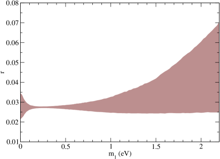
Figure 8: Effect of the perturbations on $r$ for $\kappa=0.2$, as a function of the mass of the lightest neutrino, in scenario 1.

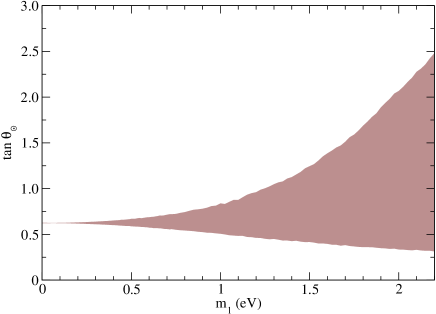
Figure 9: Effect of the perturbations on $\tan\theta_{\odot}$ for $\kappa=0.2$, as a function of the mass of the lightest neutrino, in scenario 1.

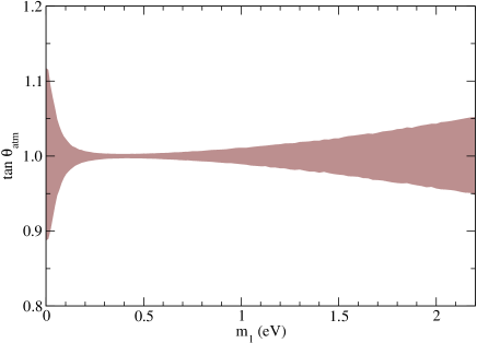
Figure 10: Effect of the perturbations on $\tan\theta_{\mathrm{atm}}$ for $\kappa=0.2$, as a function of the mass of the lightest neutrino, in scenario 1.

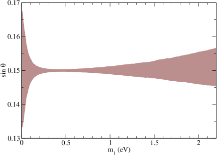
Figure 11: Effect of the perturbations on $\sin\theta$ for $\kappa=0.2$, as a function of the mass of the lightest neutrino, in scenario 1.

It is apparent that these parameters are remarkably more stable in the region around $m_{1}=0.3$ eV than for the rest of values of $m_{1}$. This can be understood as follows: the only two terms that influence the mixing are $\eta_{e}\,\hat{M}_{L}\hat{M}_{L}^{\dagger}Y^{e}$ and $\eta_{L}\left(Y^{e}Y^{e\dagger}\hat{M}_{L}+\hat{M}_{L}Y^{e*}Y^{eT}\right)$. Of these, the former is relevant only for a HI spectrum, whereas for a QD spectrum it does not have any influence. On the contrary, the latter term is important for a QD spectrum but its impact is negligible if the neutrino masses are hierarchical. Hence, the deviations in $\tan\theta_{\mathrm{atm}}$ and $\sin\theta$ appearing in the left part of Figs. 10 and 11 are due to the $\eta_{e}$ term, and the deviations in $R$, $\tan\theta_{\odot}$, $\tan\theta_{\mathrm{atm}}$ and $\sin\theta$ that can be seen in the right side of Figs. 8–11 are a consequence of the $\eta_{L}$ term. The deviations in $r$ in the left hand side of Fig. 8 is an effect of the $\zeta_{L}$ term, which does not contribute to the mixing.

The region $m\simeq 0.3$ eV is of special interest, since these neutrino masses will be probed in forthcoming experiments like KATRIN, which is planned to start in 2007. If the mass of the lightest neutrino happens to be in this range, this will mean that the corrections to the tree-level mass matrices will have a much smaller impact on the hierarchy of mass squared differences and the mixing. The same is also true for the Dirac and Majorana phases. For completeness, in Fig. 12 we show the $1\sigma$ limits on $\omega$ for the same range of $m_{1}$. We observe that this ratio remains virtually constant in the whole interval.

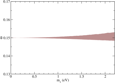
Figure 12: Effect of the perturbations on $\omega$ for $\kappa=0.2$, as a function of the mass of the lightest neutrino, in scenario 1.

For scenario 2 and for Dirac neutrinos, the dependence on the lightest neutrino mass is much simpler. For a HI spectrum, all the quantities studied are stable, and in these cases the effects of perturbations are as in Figs.  8–12 but without the deviations present in the left part of some of these plots.

IV.3 Stability of flavor relations

We are interested in finding flavor relations which are stable under perturbations of the mass matrices. By “stability” we mean that, if these relations hold for the tree-level matrices, they still hold to a good approximation when perturbations are added. With some exceptions, most flavor relations found in the literature correspond to Majorana neutrinos with a HI spectrum. In scenario 2, the parameters $r$, $\tan\theta_{\odot}$, $\tan\theta_{\mathrm{atm}}$ and $\sin\delta$, as well as the $CP$ violating phases, remain constant for a HI spectrum. Therefore, any flavor relation among these parameters is stable. In scenario 1, most of the flavor relations studied are affected by the random perturbations. For illustration, we show the effect of perturbations on some relations. For texture A1 in Ref. barbieri , there are two predictions,

$$\sin\theta = \frac{1}{2}\tan\theta_{\mathrm{atm}}\sin 2\theta_{\odot}\sqrt{r}\,,$$

$$\frac{|m_{ee}|}{m_{\mathrm{atm}}} = \sin^{2}\theta_{\odot}\sqrt{r}\,,$$ (39)

where $m_{ee}$ is the effective mass for neutrinoless double beta decay processes, and $m_{\mathrm{atm}}\equiv\sqrt{\Delta m_{\mathrm{atm}}^{2}}$. In order to test the stability of these relations under the radiative corrections considered here, we define the ratios

$$R_{\mathrm{I}} = \frac{1}{2}\frac{\tan\theta_{\mathrm{atm}}}{\sin\theta}\sin 2\theta_{\odot}\sqrt{r}\,,$$

$$R_{\mathrm{II}} = \frac{\sin^{2}\theta_{\odot}\sqrt{r}}{|m_{ee}|/m_{\mathrm{atm}}}\,,$$ (40)

which equal unity for the tree-level matrices. These ratios are plotted in Figs. 13 and 14, respectively, where we have used $\sin\theta=0.074$, $\delta=\alpha=0$, $\beta=0.85$, so that the initial matrices fulfill these relations. The rest of parameters is taken from Table 1.

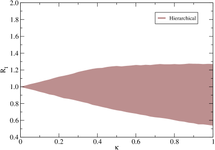
Figure 13: Effect of the perturbations on the ratio $R_{\mathrm{I}}$, in scenario 1.

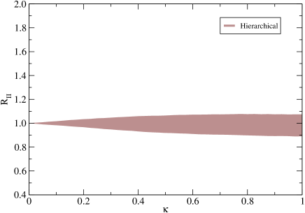
Figure 14: Effect of the perturbations on the ratio $R_{\mathrm{II}}$, in scenario 1.

From Fig. 13 we see that the first relation is modified when corrections are added to the mass matrices. At any rate, the deviations on this relation are much smaller than the changes in $r$, $\tan\theta_{\mathrm{atm}}$ and $\sin\theta$ (see Figs. 3 – 6). We also notice from Fig. 14 that the accuracy of the second relation is hardly affected by perturbations on the mass matrices. This feature makes its experimental test cleaner, and less dependent on unknown corrections to the tree-level textures. For texture B1 of Ref. barbieri (see also Ref. tanimoto ) we have

$$\sin\theta=\frac{1}{2}\tan\theta_{\mathrm{atm}}\tan 2\theta_{\odot}\sqrt{r\cos 2\theta_{\odot}}\,.$$ (41)

which differs from the first of Eqs. (39) by factors depending on $\theta_{\odot}$. Since $\theta_{\odot}$ is stable for a HI spectrum, the effect of corrections on this relation is similar, and the plot obtained is identical to Fig. 13. Another interesting relation is ross

$$\sin\theta=\sqrt{\frac{m_{e}}{m_{\mu}}}\,.$$ (42)

The left-hand side of this equation varies with the perturbations, but the right-hand side does not. We define

$$R_{\mathrm{III}}=\frac{1}{\sin\theta}\sqrt{\frac{m_{e}}{m_{\mu}}}$$ (43)

and set $\sin\theta=0.0688$ (with the rest of parameters as in Table 1) in order to test the stability of this relation. The result can be seen in Fig. 15.

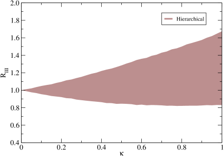
Figure 15: Effect of the perturbations on the ratio $R_{\mathrm{III}}$, in scenario 1.

The conclusion one may draw from the study of these examples is the following: if the new physics interactions are suppressed (this situation corresponds to scenario 2), the flavor relations are stable and, if they hold at tree-level, they also hold when the corrections in Eqs. (32) are included. On the other hand, if the new interactions are not suppressed and the corrections have the full form of Eqs. (30), with $\hat{M}_{L}$ of order unity (this possibility corresponds to scenario 1) some of these flavor relations are modified by the perturbations.

IV.4 Special limits

We have previously remarked that, for quasi-degenerate neutrinos, the perturbations in the mass matrices modify $\tan\theta_{\odot}$ but do not affect $\tan\theta_{\mathrm{atm}}$ significantly. Then, one interesting question naturally arises: Is it possible to have a QD spectrum with bi-maximal mixing at the tree level, so that the smaller value of $\tan\theta_{\odot}\simeq 0.6$ is due to effects of new physics? To test this hypothesis, we set $\tan\theta_{\odot}=\tan\theta_{\mathrm{atm}}=1$ in our matrices, with the rest of parameters as in Table 1, and analyze how $\tan\theta_{\odot}$ and $\tan\theta_{\mathrm{atm}}$ change when perturbations are added. For scenario 1, the results are displayed in Fig. 16. For scenario 2, the results are shown in Fig. 17.

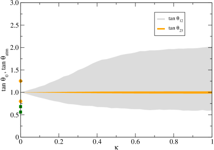
Figure 16: Effect of the perturbations on $\tan\theta_{\odot}$ and $\tan\theta_{\mathrm{atm}}$, for quasi-degenerate neutrinos and initial bi-maximal mixing, in scenario 1.

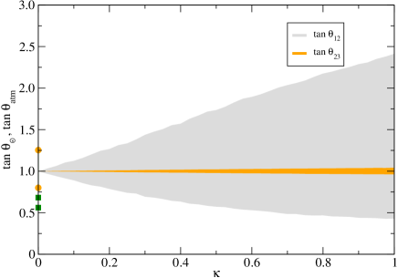
Figure 17: Effect of the perturbations on $\tan\theta_{\odot}$ and $\tan\theta_{\mathrm{atm}}$, for quasi-degenerate neutrinos and initial bi-maximal mixing, in scenario 2.

From these figures we conclude that in both scenarios it is possible that, from an initial bi-maximal pattern, large corrections to the mass matrices modify significantly $\tan\theta_{\odot}$, bringing it to its experimental value, while keeping $\tan\theta_{\mathrm{atm}}\simeq 1$. This result is only slightly dependent on the value of $\sin\theta$ used, and is valid for $m_{1}\gtrsim 0.6$ eV. For Dirac neutrinos the same effect is found, and the results are very similar to the ones in scenario 2.

Other interesting situation corresponds to $\sin\theta=0$ at the tree level. In this case, for a QD spectrum a nonzero $\sin\theta$ can be generated by the perturbations. If the neutrino masses are hierarchical, the value of $\sin\theta$ induced by the corrections is negligible. The results for scenarios 1 and 2 are displayed in Figs. 18 and 19, respectively. For Dirac neutrinos, the value of $\sin\theta$ generated is one order of magnitude smaller.

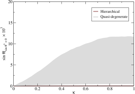
Figure 18: Effect of the perturbations on $\sin\theta$, for an initial vanishing value, in scenario 1.

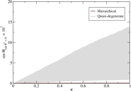
Figure 19: Effect of the perturbations on $\sin\theta$, for an initial vanishing value, in scenario 2.

Finally, we consider the situation when $\delta=0$ at the tree level but the Majorana phases are not zero. In this limit, the $CP$ violating parameter $\mathcal{J}$ in Eq. (17) vanishes. For a QD spectrum, the corrections to the mass matrices induce a Dirac phase (provided at least one of the Majorana phases is nonzero) large enough to yield $\mathcal{J}\sim 10^{-2}$, which may be observable by future long baseline neutrino oscillation experiments Lindner:2002vt . This is shown in Figs. 20 and 21, and holds for $m_{1}\gtrsim 0.7$ eV. Setting one of the initial Majorana phases to zero does not eliminate this effect, and for $\alpha=\pi/3$, $\beta=0$ the values of $\mathcal{J}$ obtained are up to 0.02, even larger than the ones shown in Figs. 20 and 21. For a HI spectrum, the phase $\delta$ generated is negligible. In the case of Dirac neutrinos, only the Dirac phase is physically meaningful, and the phases of the random parameters $\lambda_{i}$, $\zeta_{i}$ and $\eta_{i}$ are not enough to produce a relevant value of $\mathcal{J}$.

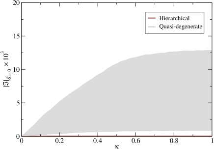
Figure 20: Effect of the perturbations on $\mathcal{J}$, for an initial vanishing Dirac phase, in scenario 1.

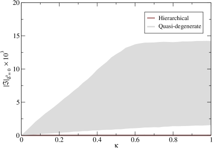
Figure 21: Effect of the perturbations on $\mathcal{J}$, for an initial vanishing Dirac phase, in scenario 2.

V Outlook

In this paper we have studied the possible effect of unknown corrections from new physics on the neutrino mass hierarchy, mixing and $CP$ violation at low energies. We have focused on the case when neutrinos are Majorana particles, but have discussed the results for Dirac neutrinos as well. We have proposed a general parametrization of the corrections to the tree-level mass matrices, based on weak basis invariance. Using this parametrization, we have examined the consequences of adding random perturbations to the mass matrices, as a means to explore the possible effects that radiative corrections might yield.

We have analyzed the stability against corrections of the ratio of mass squared differences and the mixing angles, for a hierarchical or quasi-degenerate neutrino spectrum. We have found that these quantities are generally modified by the perturbations, but the ratio $\omega=\sin\theta/\sin\theta_{\mathrm{atm}}$ is remarkably stable even under large corrections. This desirable property makes this quantity specially suited for the experimental test of specific textures of neutrino mass matrices, since it is hardly modified by unknown corrections to the tree-level matrices. We have also examined the stability of some flavor relations predicted by models in the literature.

The dependence of the deviations on the neutrino spectrum has also been investigated. We have found that the region of neutrino masses $m\simeq 0.3$ eV is specially stable. For neutrino masses around this value, the possible deviations in $r$, $\tan\theta_{\odot}$, $\tan\theta_{\mathrm{atm}}$, $\sin\theta$ and the $CP$ violating phases are rather small. This mass region is of special interest, since it will be tested in upcoming experiments.

We have addressed the question whether the tree-level mass matrices could correspond to bi-maximal mixing, being the observed value $\tan\theta_{\odot}\sim 0.6$ the result of radiative corrections. We have demonstrated that, from an initial bi-maximal pattern, in the case of a QD spectrum the corrections to the mass matrices can bring down $\tan\theta_{\odot}$ to its experimental value while keeping $\tan\theta_{\mathrm{atm}}$ very close to unity. This result holds both for Majorana and Dirac neutrinos, and for a lightest neutrino with a mass larger than $\simeq 0.6$ eV. Therefore, the possibility of bi-maximal mixing cannot be excluded for a QD spectrum. On the other hand, for a HI spectrum $\tan\theta_{\mathrm{atm}}$ is modified but $\tan\theta_{\odot}$ not, then bi-maximal mixing is highly unlikely in this case.

Other interesting limit examined is when $\sin\theta=0$ at the tree level. In this case, large corrections to the mass matrices could yield $\sin\theta\sim 10^{-2}$ if the neutrinos are quasi-degenerate. On the contrary, we have shown that for a HI spectrum or Dirac neutrinos the value of $\sin\theta$ generated by perturbations is negligible.

Finally, we have investigated the situation when the Dirac phase in the mixing matrix vanishes at the tree level. In this case, the Majorana phases present can induce a non-vanishing Dirac phase in the mixing matrix by means of the perturbations. This Dirac phase is large enough to yield $\mathcal{J}\gtrsim 10^{-2}$, leading to observable $CP$ violation effects in long baseline neutrino oscillation experiments.

- (1) M. Gell-Mann, P. Ramond and R. Slansky, in Supergravity, ed. by P. van Nieuwenhuizen and D. Z. Freedman (North Holland, Amsterdam, 1979), p.315.
- (2) S. L. Glashow, in Quarks and Leptons, Cargèse, 1979, edited by M. Levy et al. (Plenum, New York, 1980).
- (3) T. Yanagida, in Proc. of the Workshop on the Unified Theory and Baryon Number in the Universe, ed. by O. Sawada and A. Sugamoto (KEK report 79-18, 1979), p.95, Tsukuba, Japan.
- (4) R. N. Mohapatra and G. Senjanovic, Phys. Rev. Lett. 44, 912 (1980).
- (5) T. P. Cheng and L. F. Li, Phys. Rev. D 22, 2860 (1980).
- (6) G. B. Gelmini and M. Roncadelli, Phys. Lett. B 99, 411 (1981).
- (7) C. Wetterich, Nucl. Phys. B 187, 343 (1981).
- (8) A. Rossi, Phys. Rev. D 66, 075003 (2002) [hep-ph/0207006].
- (9) For a recent work see e.g. M. A. Díaz, M. Hirsch, W. Porod, J. C. Romão and J. W. Valle, Phys. Rev. D 68, 013009 (2003) [hep-ph/0302021], and references therein.
- (10) J. A. Casas, J. R. Espinosa and I. Navarro, Phys. Rev. Lett. 89, 161801 (2002) [hep-ph/0206276].
- (11) M. Roncadelli and D. Wyler, Phys. Lett. B 133, 325 (1983).
- (12) P. Roy and O. Shanker, Phys. Rev. Lett. 52, 713 (1984) [Erratum-ibid. 52, 2190 (1984)].
- (13) D. Chang and R. N. Mohapatra, Phys. Rev. Lett. 58, 1600 (1987).
- (14) M. Lindner, T. Ohlsson and G. Seidl, Phys. Rev. D 65, 053014 (2002) [hep-ph/0109264].
- (15) I. Gogoladze and A. Pérez-Lorenzana, Phys. Rev. D 65, 095011 (2002) [hep-ph/0112034].
- (16) K. R. Dienes, E. Dudas and T. Gherghetta, Nucl. Phys. B 557, 25 (1999) [hep-ph/9811428].
- (17) A. E. Faraggi and M. Pospelov, Phys. Lett. B 458, 237 (1999) [hep-ph/9901299].
- (18) D. O. Caldwell, R. N. Mohapatra and S. J. Yellin, Phys. Rev. Lett. 87, 041601 (2001) [hep-ph/0010353].
- (19) G. Barenboim, G. C. Branco, A. de Gouvea and M. N. Rebelo, Phys. Rev. D 64, 073005 (2001) [hep-ph/0104312].
- (20) H. Davoudiasl, P. Langacker and M. Perelstein, Phys. Rev. D 65, 105015 (2002) [hep-ph/0201128].
- (21) P. Q. Hung, Phys. Rev. D 67, 095011 (2003) [hep-ph/0210131].
- (22) See e.g. H. Fritzsch and J. Plankl, Phys. Lett. B 237, 451 (1990); K. S. Babu and S. M. Barr, Phys. Lett. B 381, 202 (1996) [hep-ph/9511446]; C. Jarlskog, M. Matsuda, S. Skadhauge and M. Tanimoto, Phys. Lett. B 449, 240 (1999) [hep-ph/9812282]; M. Jezabek and Y. Sumino, Phys. Lett. B 457, 139 (1999) [hep-ph/9904382]; G. C. Branco, M. N. Rebelo and J. I. Silva-Marcos, Phys. Rev. D 62, 073004 (2000) [hep-ph/9906368]; G. Altarelli, F. Feruglio and I. Masina, Phys. Lett. B 472, 382 (2000) [hep-ph/9907532]; H. Fritzsch and Z. z. Xing, Prog. Part. Nucl. Phys. 45, 1 (2000) [hep-ph/9912358]; E. K. Akhmedov, G. C. Branco, F. R. Joaquim and J. I. Silva-Marcos, Phys. Lett. B 498, 237 (2001) [hep-ph/0008010]; G. C. Branco and J. I. Silva-Marcos, Phys. Lett. B 526, 104 (2002) [hep-ph/0106125]; R. González Felipe and F. R. Joaquim, JHEP 0109, 015 (2001) [hep-ph/0106226]; S. F. King and G. G. Ross, Phys. Lett. B 520, 243 (2001) [hep-ph/0108112]; C. D. Froggatt, H. B. Nielsen and Y. Takanishi, Nucl. Phys. B 631, 285 (2002) [hep-ph/0201152]; K. S. Babu and R. N. Mohapatra, Phys. Lett. B 532, 77 (2002) [hep-ph/0201176]; F. S. Ling and P. Ramond, Phys. Lett. B 543, 29 (2002) [hep-ph/0206004]; S. Raby, Phys. Lett. B 561, 119 (2003) [hep-ph/0302027].
- (23) For reviews see e.g. G. Altarelli and F. Feruglio, Phys. Rept. 320, 295 (1999); I. Masina, Int. J. Mod. Phys. A 16, 5101 (2001) [hep-ph/0107220]; M. C. Gonzalez-Garcia and Y. Nir, Rev. Mod. Phys. 75, 345 (2003) [hep-ph/0202058]; V. Barger, D. Marfatia and K. Whisnant, hep-ph/0308123; S. F. King, hep-ph/0310204.
- (24) L. J. Hall, H. Murayama and N. Weiner, Phys. Rev. Lett. 84, 2572 (2000) [hep-ph/9911341].
- (25) F. Vissani, Phys. Lett. B 508, 79 (2001) [hep-ph/0102236].
- (26) G. Altarelli, F. Feruglio and I. Masina, JHEP 0301, 035 (2003) [hep-ph/0210342].
- (27) J. R. Espinosa, hep-ph/0306019.
- (28) J. A. Aguilar-Saavedra, Phys. Rev. D 67, 073026 (2003) [hep-ph/0212057].
- (29) See C. Giunti and M. Laveder, hep-ph/0310238, and references therein.
- (30) K. Eguchi et al. [KamLAND Collaboration], Phys. Rev. Lett. 90 (2003) 021802 [hep-ex/0212021].
- (31) M. Guzzo, P. C. de Holanda, M. Maltoni, H. Nunokawa, M. A. Tortola and J. W. Valle, Nucl. Phys. B 629 (2002) 479 [hep-ph/0112310 v3 KamLAND updated version].
- (32) J. Barranco, O. G. Miranda, T. I. Rashba, V. B. Semikoz and J. W. Valle, Phys. Rev. D 66 (2002) 093009 [hep-ph/0207326 v3 KamLAND updated version].
- (33) S. N. Ahmed et al. [SNO Collaboration], nucl-ex/0309004.
- (34) A. B. Balantekin and H. Yuksel, hep-ph/0309079.
- (35) G. L. Fogli, E. Lisi, A. Marrone and A. Palazzo, hep-ph/0309100.
- (36) M. Maltoni, T. Schwetz, M. A. Tortola and J. W. Valle, hep-ph/0309130.
- (37) P. Aliani, V. Antonelli, M. Picariello and E. Torrente-Lujan, hep-ph/0309156.
- (38) A. Bandyopadhyay, S. Choubey, S. Goswami, S. T. Petcov and D. P. Roy, hep-ph/0309174.
- (39) P. Creminelli, G. Signorelli and A. Strumia, JHEP 0105 (2001) 052 [hep-ph/0102234 v5].
- (40) P. C. de Holanda and A. Y. Smirnov, hep-ph/0309299.
- (41) Y. Fukuda et al. [Super-Kamiokande Collaboration], Phys. Rev. Lett. 81 (1998) 1562 [hep-ex/9807003].
- (42) M. H. Ahn et al. [K2K Collaboration], Phys. Rev. Lett. 90 (2003) 041801 [hep-ex/0212007].
- (43) J. Bonn et al., Prog. Part. Nucl. Phys. 48, 133 (2002).
- (44) V. M. Lobashev et al., Nucl. Phys. Proc. Suppl. 91, 280 (2001).
- (45) For updated analyses see e.g. F. R. Joaquim, Phys. Rev. D 68, 033019 (2003) [hep-ph/0304276]; H. Murayama and C. Peña-Garay, hep-ph/0309114; S. Pascoli and S. T. Petcov, hep-ph/0310003 and also F. Feruglio, A. Strumia and F. Vissani, Nucl. Phys. B 637, 345 (2002) [Addendum-ibid. B 659, 359 (2003)] [hep-ph/0201291 v5].
- (46) G. L. Fogli, E. Lisi, A. Marrone and D. Montanino, Phys. Rev. D 67, 093006 (2003) [hep-ph/0303064].
- (47) M. Apollonio et al. [CHOOZ Collaboration], Phys. Lett. B 466, 415 (1999) [hep-ex/9907037].
- (48) G. L. Fogli, E. Lisi, A. Marrone, D. Montanino, A. Palazzo and A. M. Rotunno, Phys. Rev. D 67, 073002 (2003) [hep-ph/0212127].
- (49) M. Lindner, hep-ph/0209083.
- (50) S. Weinberg, Phys. Rev. D 22, 1694 (1980).
- (51) M. Frigerio and A. Y. Smirnov, JHEP 0302, 004 (2003). [hep-ph/0212263]
- (52) H. Fusaoka and Y. Koide, Phys. Rev. D 57, 3986 (1998) [hep-ph/9712201].
- (53) For analyses on the impact of RG corrections in neutrino masses and mixing see e.g. P. H. Chankowski and S. Pokorski, Int. J. Mod. Phys. A 17, 575 (2002) [hep-ph/0110249]; S. Antusch, J. Kersten, M. Lindner and M. Ratz, hep-ph/0305273, and references therein.
- (54) R. Barbieri, T. Hambye and A. Romanino, JHEP 0303, 017 (2003) [hep-ph/0302118].
- (55) M. Honda, S. Kaneko and M. Tanimoto, JHEP 0309, 028 (2003) [hep-ph/0303227].
- (56) G. G. Ross and L. Velasco-Sevilla, Nucl. Phys. B 653, 3 (2003) [hep-ph/0208218].