Modeling quark-hadron duality for relativistic, confined fermions

Abstract

We discuss a model for the study of quark-hadron duality in inclusive electron scattering based on solving the Dirac equation numerically for a scalar confining linear potential and a vector color Coulomb potential. We qualitatively reproduce the features of quark-hadron duality for all potentials considered, and discuss similarities and differences to previous models that simplified the situation by treating either the quarks or all particles as scalars. We discuss the scaling results for PWIA and FSI, and the approach to scaling using the analog of the Callan-Gross relation for y-scaling.

I Introduction

Quark-hadron duality was first discovered experimentally in inclusive inelastic electron scattering by Bloom and Gilman bgduality , more than 30 years ago. In the past few years, quark-hadron duality has generated a lot of interest both on the experimental jlab ; prdmom and on the theoretical side closeisgur ; closezhao ; closewallym ; pp ; mpdirac ; pps ; donghe ; dongli ; kiev ; leyaouancped ; simula ; ijmvo ; jvod2 ; elba . Duality is a major point in the planned 12 GeV upgrade of CEBAF at Jefferson Lab 12gevwp . It is also the basis for using QCD sum rules qcdsr , and plays an important role in the study of semileptonic decays of heavy mesons richural ; semilep .

Quark-hadron duality implies that in certain kinematic regions, the appropriate average of hadronic observables is described by a perturbative quantum chromodynamics (pQCD) result. This is of great practical interest, as we are actually able to carry out a perturbative QCD calculation, in contrast to a full QCD or full hadronic calculation. Surprisingly, duality was experimentally shown to hold in inclusive inelastic electron scattering down to momentum transfers of $Q^{2}\approx 0.5$ GeV² jlab . Duality also holds in the semi-leptonic decay of heavy quarks isgurwise , and in the annihilation $e^{+}e^{-}\rightarrow hadrons$. The exact manner of averaging depends on the process.

Duality is not only a very interesting phenomenon by itself, but it also has extremely important applications. As duality connects the resonance region, i.e. the region where the final state invariant mass $W<2$ GeV, and the deep inelastic region, one may infer information on one from the other. The earliest example discussed was the extraction of the elastic nucleon form factor from the deep inelastic scaling curve dgp . In jiunrau , higher twist contributions were inferred from the resonance data. This connection afforded by duality opens up the large $x_{Bj}$ regime experimentally, as higher $Q^{2}$ measurements are difficult to obtain - note that the $(e,e^{\prime})$ cross section contains the Mott cross section as a factor, and the Mott cross section is proportional to $1/Q^{4}$. The large $x_{Bj}$ region is much easier to access in the resonance region, as the necessary $Q^{2}$ values there are much smaller.

One of the most exciting and promising applications of duality will be the measurement of the neutron polarization asymmetry $A_{1}^{n}$ at large $x_{Bj}$. There are many different theoretical predictions for this quantity, ranging from 0 (unbroken SU(6)) to 1 (pQCD) nathana1n . Experimental information on $A_{1}^{n}$ at large $x_{Bj}$ would greatly enhance our understanding of the valence quark spin distribution functions. There are very recent new data from Jefferson Lab, going up to $x_{Bj}=0.6$ a1data , with small error bars, but the deep valence region of $x_{Bj}\to 1$ remains inaccessible in deep inelastic scattering. If duality is well understood, one may take data in the resonance region, apply a proper averaging procedure, and thus obtain results for $A_{1}^{n}(x_{Bj}\rightarrow 1)$.

New theoretical approaches to a better understanding of duality have been based on modeling: one branch uses the non-relativistic constituent quark model, with some relativistic corrections, to describe duality closeisgur ; closewallym ; donghe ; dongli , and another branch starts the modeling with a relativistic one-body equation closezhao ; pp ; mpdirac ; pps ; ijmvo ; jvod2 . The former branch makes contact with the phenomenology. It was started by the pioneering work of Close and Isgur closeisgur , where the authors investigated how a summation over the appropriate sets of nucleon resonances leads to parton model results for the structure function ratios in the SU(6) symmetric quark model. This work was recently expanded closewallym to include the effects of SU(6) spin-flavor symmetry breaking. In donghe ; dongli , the authors considered the first five low-lying resonances. Our results belong to the latter branch. The goal of these modeling efforts is obvious: to gain an understanding of quark-hadron duality and the conditions under which it holds, by capturing just the essential physical conditions of this rather complex phenomenon. We imposed these basic requirements for a model: we require a relativistic description of confined valence quarks, and we treat the hadrons in the infinitely narrow resonance approximation.

This paper is the third in a series on modeling quark-hadron duality in inclusive electron scattering - the reaction in which quark-hadron duality was first observed by Bloom and Gilman. Previously, we simplified the situation by first assuming that all particles involved are scalars ijmvo , and then relaxed these constraints for beam electrons and exchange photons, and only assumed scalar quarks jvod2 . While these simplifications are physically significant, they allowed us to calculate all interesting quantities analytically or semi-analytically. We found that the features of quark-hadron duality were reproduced qualitatively in both models. Now, we have taken one more step towards a realistic description of the problem: previously, we simplified the problem by discussing scalar quarks, but now, we use proper spin-1/2 quarks in our model. This lays the foundation for investigating duality in polarization observables.

Also, for the first time, in this paper we present calculations for three different confining potentials. Previously, we used a linear potential in the Klein-Gordon equation, which leads to a ”relativistic oscillator”. Now, we present a scalar linear confining potential and combine it with a vector potential: either with a static color Coulomb potential or with a running color Coulomb potential.

The paper is organized as follows: first, we introduce the model and then give model results in PWIA. The next section discusses y-scaling: the connection between y-scaling and Bjorken scaling, y-scaling results from our two previous models, y-scaling in PWIA and FSI, and the sensitivity to different potentials. Then, we discuss our results for sum rules in PWIA and FSI. In the next section, we derive the analog of the Callan-Gross relation for y-scaling, and investigate the onset of scaling through this relation. Then, we summarize our results and give a brief outlook.

II The Model

Our model consists of a constituent quark bound to an infinitely heavy di-quark and is represented by the Dirac hamiltonian

$$\hat{H}=\bm{\alpha}\cdot\hat{\bm{p}}+\beta\left(m+V_{s}(r)\right)+V_{v}(r)\,,$$ (1)

where the scalar potential is a linear confining potential given by

$$V_{s}(r)=br,\qquad\qquad b=0.18{\rm GeV}^{2}\,.$$ (2)

We have used the constituent quark mass in this paper, as our main interest is the study of quark-hadron duality, which sets in at rather low $Q^{2}$, experimentally $Q^{2}\approx 0.5~{}GeV^{2}$ is enough. In this kinematic region, the appropriate degree of freedom is the constituent quark, which has acquired mass through spontaneous chiral symmetry breaking. We have used a value for the quark mass of $m=258.46~{}MeV$ - obtained previously in a fit to heavy mesons waw . Calculations will be presented where the vector color Coulomb potential is absent, that is $V_{c}(r)=0$, where the vector potential is the simple static Coulomb potential

$$V_{c}(r)=-\frac{4}{3}\frac{\alpha_{s}}{r}$$ (3)

with $\alpha_{s}=0.181$ and where the color Coulomb potential is corrected to allow for the running coupling constant in a manner similar to that used by Godfrey and Isgur godfreyisgur . This potential has the form

$$V_{cr}(r)=-\frac{4}{3r}\left(\alpha_{c}\frac{1+e^{-}\frac{\rho_{0}}{\delta}}{1+e^{\frac{\sqrt{b}r-\rho_{0}}{\delta}}}+\sum_{i=1}^{2}\alpha_{i}{\rm erf}(\gamma_{i}r)\right)$$ (4)

where

$$\alpha_{c} = 0.118$$

$$\rho_{0} = 0.04$$

$$\delta = 0.01$$

$$\alpha_{1} = 0.239$$

$$\alpha_{2} = 0.271$$

$$\gamma_{1} = 0.746\ {\rm GeV}$$

$$\gamma_{2} = 5.40\ {\rm GeV}$$ (5)

We assume that only the light quark carries a charge, and we choose unit charge for the light quark for simplicity. The inclusive cross section is given by the usual Rosenbluth equation

$$\frac{d^{2}\sigma}{d\Omega dE}=\sigma_{\rm Mott}\left\{\frac{Q^{4}}{\bm{q}^{4}}R_{L}(q,\nu)+\left(\frac{Q^{2}}{2\bm{q}^{2}}+\tan^{2}\frac{\theta}{2}\right)R_{T}(q,\nu)\right\}\,,$$ (6)

where $\sigma_{\rm Mott}$ is the Mott cross section, $\bm{q}$ is the three-momentum transfer from the electron to the target, $\nu$ is the energy transfer and $Q^{2}=\bm{q}^{2}-\nu^{2}$. The longitudinal and transverse response functions for the model are given by

$$R_{L}(q,\nu)=\sum_{f}\left|\left<\Psi_{f}\right|e^{i\bm{q}\cdot\bm{r}}\left|\Psi_{0}\right>\right|^{2}\delta\left(\nu+E_{0}-E_{f}\right)$$ (7)

and

$$R_{T}(q,\nu)=\sum_{f}\sum_{i=1}^{2}\left|\left<\Psi_{f}\right|e^{i\bm{q}\cdot\bm{r}}\alpha_{i}\left|\Psi_{0}\right>\right|^{2}\delta\left(\nu+E_{0}-E_{f}\right)\,,$$ (8)

where $E_{0}$ is the ground state energy. In terms of these response functions the structure functions are

$$W_{1}(Q^{2},\nu)=\frac{1}{2}R_{T}(q,\nu)$$ (9)

and

$$W_{2}(Q^{2},\nu)=\frac{Q^{4}}{\bm{q}^{4}}R_{L}(q,\nu)+\frac{Q^{2}}{2\bm{q}^{2}}R_{T}(q,\nu)\,.$$ (10)

The Dirac wave functions and energy eigenvalues are obtained by integrating the Dirac equation using the Runge-Kutta-Feldberg technique and solutions are obtained for energies up to 12 GeV with the radial quantum number of $n\cong 200$ and $|\kappa|\leq 70$.

In our model, we excite the bound quark from the ground state to higher energy states, and do not allow it to decay. Thus, we do not include any particle production in our model, and are strictly quantum-mechanical in this sense. We do not have any gluons in our model, either, which means that we do not encounter any radiative corrections. Since the response functions consist of a sum of delta functions, we choose to smear out the response functions by folding with a narrow gaussian for purposes of visualization. The smeared response functions are then given by

$$R_{L(T)}(q,\nu)=\frac{1}{\sqrt{\pi}\epsilon}\int_{-\infty}^{\infty}d\nu^{\prime}\,e^{-\frac{(\nu-\nu^{\prime})^{2}}{\epsilon^{2}}}R_{L(T)}^{unsmeared}(q,\nu^{\prime})\,.$$ (11)

Before presenting numerical results, we would like to remind our readers that, while the present model is more realistic than its predecessors, its results should not be compared quantitatively to inclusive electron scattering from a nucleon. Due to the assumption of an infinitely heavy antiquark (or diquark) to which the light quark is bound, our calculation most resembles inclusive electron scattering from a B-meson, which has never been measured. However, the goal of our work is to gain a qualitative understanding of duality, and the current simplification is no impediment to this.

III The Plane Wave Impulse Approximation

The analog to pQCD for this model is the plane wave impulse approximation where the bound quark is knocked into the continuum by the absorption of the virtual photon. The response tensor for this approximation is

$$W^{\mu\nu} = \frac{1}{8}\int\frac{d^{3}p}{(2\pi)^{3}}\frac{m}{E_{\bm{p}+\bm{q}}}\delta(\nu+E_{0}-E_{\bm{p}+\bm{q}})$$ (12)

$$\times{\rm Tr}\left[\gamma^{\mu}\frac{\gamma\cdot(p+q)+m}{2m}\,\gamma^{\nu}\left(\gamma\cdot n_{v}(p)+n_{s}(p)\right)\right]$$

where the vector and scalar momentum density distributions $n_{v}(p)$ and $n_{s}(p)$ are defined in terms of the ground state wave function

$$\Psi_{10\frac{1}{2}m}(\bm{p})=\left(\begin{array}[]{c}\psi^{(+)}_{10\frac{1}{2}}(p){\cal Y}_{0\frac{1}{2}}^{m}(\Omega_{p})\\ \psi^{(-)}_{10\frac{1}{2}}(p){\cal Y}_{1\frac{1}{2}}^{m}(\Omega_{p})\end{array}\right)$$ (13)

as

$$n_{v}(p)=\left(n_{v}^{0}(p),\frac{\bm{p}}{|\bm{p}|}n_{v}^{s}(p)\right)$$ (14)

with

$$n_{v}^{0}(p)=\frac{1}{2\pi}\left({\psi^{(+)}_{10\frac{1}{2}}}^{2}(p)+{\psi^{(-)}_{10\frac{1}{2}}}^{2}(p)\right)$$ (15)

and

$$n_{v}^{s}(p)=\frac{1}{\pi}\psi^{(+)}_{10\frac{1}{2}}(p)\psi^{(-)}_{10\frac{1}{2}}(p)\,;$$ (16)

and

$$n_{s}(p)=\frac{1}{2\pi}\left({\psi^{(+)}_{10\frac{1}{2}}}^{2}(p)-{\psi^{(-)}_{10\frac{1}{2}}}^{2}(p)\right)\,.$$ (17)

After performing the angular integrals, the response functions can be written as

$$R_{L}(q,\nu) = \frac{1}{16\pi^{2}q}\int^{y+2q}_{|y|}dp\,p\biggl{\{}(\nu+E_{0})n_{v}^{0}(p)+mn_{s}(p)$$ (18)

$$+\left.\frac{(\nu+E_{0})^{2}+p^{2}-q^{2}-m^{2}}{2p}n_{v}^{s}(p)\right\}$$

and

$$R_{T}(q,\nu) = \frac{1}{8\pi^{2}q}\int^{y+2q}_{|y|}dp\,p\biggl{\{}(\nu+E_{0})n_{v}^{0}(p)-mn_{s}(p)$$ (19)

$$-\left.\frac{(\nu+E_{0})^{2}-p^{2}+q^{2}-m^{2}}{2q}\ \frac{(\nu+E_{0})^{2}-p^{2}-q^{2}-m^{2}}{2pq}n_{v}^{s}(p)\right\}\,,$$

where

$$y=\sqrt{(\nu+E_{0})^{2}-m^{2}}-q\,.$$ (20)

IV y Scaling

Duality implies that we see scaling at high enough energy and momentum transfers, and that the results in the resonance region, for lower momentum transfers, oscillate around this scaling curve jlab . So, the first point that needs to be checked is the onset of scaling in our model. For our previous two models, we were able to show analytically that there is scaling, and that the scaling curves for PWIA and FSI coincide exactly. This result is in contrast to pp , where a $30\%$ difference was found between the PWIA and FSI scaling curves. In pp , a different one-body equation, a semi-relativistic Hamiltonian of the form $H=\sqrt{|\bm{p}|^{2}}+\sqrt{\sigma}r$ for massless quarks was used, whereas we have used a Klein-Gordon equation in our previous modeling, appropriate for spinless “quarks” with mass. Now that we use the Dirac equation, we will again have to investigate the important question if the two scaling curves coincide or not. The scaling behavior, and a possible violation of “FSI scaling curve = PWIA scaling curve” would have implications for our interpretation of deep inelastic scattering data, where one usually assumes that FSI can be neglected. The question if and how scaling may arise in the presence of FSI has been discussed in the literature before, both for non-relativistic greenberg ; gurvitzrinat ; harrington and relativistic lps approaches. Here, we are interested in duality, and need to compare the FSI scaling results with the PWIA scaling results.

Note that there is a certain arbitrariness in defining “scaling” - have we reached scaling only once all curves coincide perfectly, or is a minimal shift in the curves when, e.g., doubling the momentum, enough? In the following, our usage is that “scaling” is reached when the change in the curve is minimal for a very substantial change in the momentum transfer.

IV.1 Bjorken scaling and y-scaling

In our two previous papers on modelling duality ijmvo ; jvod2 , we have presented our results for the scaling functions at fixed $Q^{2}$ as functions of a scaling variable $u$. In the Bjorken limit, $Q^{2}\to\infty$, $u$ goes to $u_{Bj}=\frac{M}{m}x_{Bj}$, where $x_{Bj}=\frac{Q^{2}}{2M\nu}$ is Bjorken’s scaling variable, and $u_{Bj}$ is the appropriately rescaled version of $x_{Bj}$ for the case of a a target with infinite mass $M$. The values of the energy transfer $\nu$ accessed for various, fixed values of $Q^{2}$ are shown in Fig. 1 in the left panel.

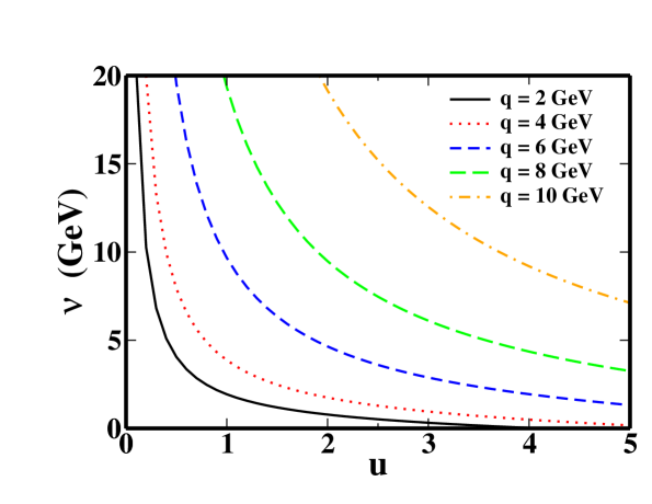
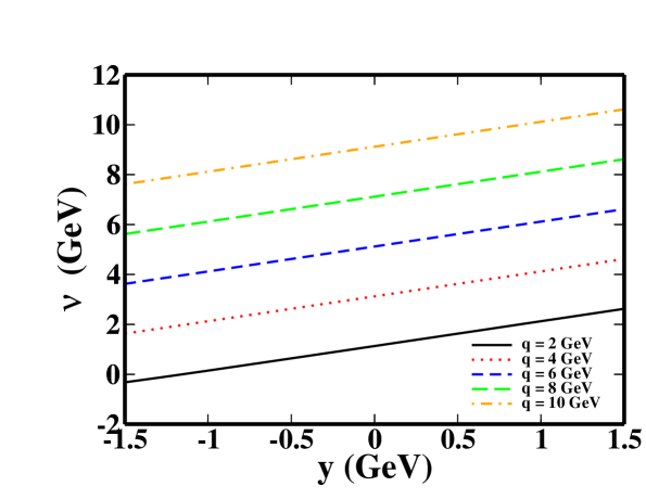
Figure 1: The transferred energy $\nu$ as a function of the scaling variable $u$ for various values of the four-momentum transfer $Q^{2}$ (top panel), and as a function of the scaling variable $y$ for various values of the three-momentum transfer $q$ (bottom panel).

We would like to point out that the previously used simplification of modelling the quark as a scalar has allowed us to obtain analytic results for the structure functions, giving us access to high energy transfers and high $Q^{2}$ without any practical, numerical problems. Now, however, we have to rely on a solely numerical solution of the Dirac equation, and cannot push to arbitrarily high $Q^{2}$ and $\nu$ values anymore. In particular, we find about 28000 energy eigenstates, all below $12~{}GeV$ energy. While this is an impressive number of states, it is clear from Fig. 1 that we will not be able to reach the high $Q^{2}$ values found necessary for scaling in our model jvod2 with energy transfers of less than $12~{}GeV$. Note that the peak of the structure function $\nu W_{2}$ is localized around $u\approx 2-3$, so the higher $Q^{2}$ values accessible at larger $u$ have little practical significance.

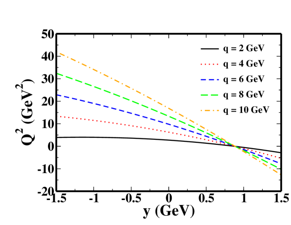
Figure 2: The transferred four-momentum $Q^{2}$ as a function of the scaling variable $y$ for various values of the three-momentum transfer $q$.

The matrix elements take their simplest form if calculated as functions of $q$. Therefore, we consider y-scaling in this paper, and use the scaling variable as defined in Eq.(20),

$$y=\sqrt{(\nu+E_{0})^{2}-m^{2}}-q\,.$$

This variable leads to scaling for fixed $|\bf{q}|$ $=q$ elba . The kinematics accessed in a y-scaling analysis are shown in Figs. 1 and 2. Fig. 1, bottom panel, shows the values of the energy transfer $\nu$ accessed in the range from $y=-2~{}GeV$ to $y=2~{}GeV$ - this is the range in which we have non-negligible contributions to our response functions and structure functions. Fig. 2 shows that we are now probing a different kinematic region than in $u$-scaling: we access both spacelike and timelike values of the four-momentum transfer $Q^{2}$. At lower, negative $y$ values, $Q^{2}$ is spacelike and rather large. In this region, we can easily reach large values associated with scaling in $u$ or $x$-type variables. The accessed $Q^{2}$ values decrease slowly with increasing $y$, and at a point where $y_{0}=E_{0}+O(\frac{1}{q})$, we reach the photopoint, $Q^{2}=0$. Note that due to the fact that $y_{0}$ is independent of $q$ in first approximation, the photopoint is reached at the same $y$ value independent of the considered three-momentum transfer $q$. For $y>y_{0}$, we probe the timelike region. Note that one also reaches timelike values of $Q^{2}$ for $y<-2q-E_{0}+O(\frac{1}{q})$; in this region, however, we find zero strength of the responses, and it is practically irrelevant for our case.

IV.2 Comparison with previous results

In order to provide a connection between $u$-scaling and $y$-scaling, we show our results for our two previous models with scalar quarks for $y$-scaling. We start out with the all-scalar results discussed in ijmvo . In ijmvo , we treated beam, exchange particle and quark target as scalars. This simplified treatment allows for an analytic solution of the problem. With all particles being scalars, only one structure function appears, there is little structure, and scaling sets in around $Q^{2}\approx 15~{}GeV^{2}$. Scaling for the PWIA sets in at very low $Q^{2}$ of about $2~{}GeV^{2}$. Keep in mind that we scatter from an infinitely heavy target, so that a comparison of numerical values for $Q^{2}$ for the onset of scaling with actual nucleon data is meaningless.

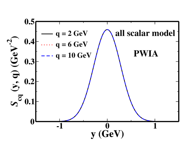
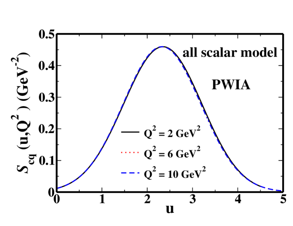
Figure 3: The scaling function ${\cal{S}}_{cq}$ of the all-scalar model ijmvo is plotted versus $y$ for several values of the three-momentum transfer $q$ in the top panel, and it is plotted versus $u$ for several values of the four-momentum transfer $Q^{2}$ in the bottom panel. The results shown have been calculated in PWIA.

Fig. 3 (top panel) shows the corresponding $y$-scaling plot for the PWIA. One can see clearly that for $q=2~{}GeV$, scaling has already set in. Obviously, there are no resonance bumps in the PWIA plot, as the final state is a fictitious “free quark”. In the bottom panel of Fig. 3, we show the same PWIA scaling function, plotted for fixed four-momentum transfer $Q^{2}$ versus $u$. The overall features of the curves, plotted either way, are the same: they are smooth and scale quickly. In the $u$-scaling plot, one sees that scaling has set in at $Q^{2}=6~{}GeV^{2}$, and the changes from the lower value of $Q^{2}=2~{}GeV^{2}$ to $Q^{2}=6~{}GeV^{2}$ are tiny.

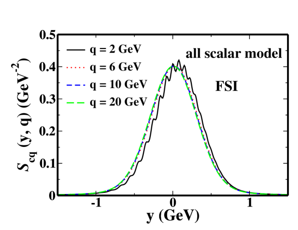
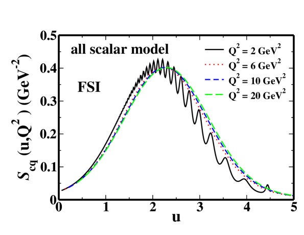
Figure 4: The scaling function ${\cal{S}}_{cq}$ of the all-scalar model is plotted versus $y$ for several values of the three-momentum transfer $q$ in the top panel, and it is plotted versus $u$ for several values of the four-momentum transfer $Q^{2}$ in the bottom panel. The results shown have been calculated including final state interactions (FSI).

Fig. 4, top panel, shows the $y$-scaling plot for the all-scalar model including FSI. Here, one can see that scaling does take a while to set in - the lowest value for $q$ that is displayed, $q=2~{}GeV$, still shows the typical resonance bump structure. However, the overall shape even at low $q$ is already very close to the scaling curve, but slightly shifted towards higher $y$ values. The scaling curve is approximated reasonably at $q=6~{}GeV$, and the curves start to coincide with each other once $q=10~{}GeV$ is reached.

This is contrasted with the $u$-scaling plot for the all-scalar model including FSI in the bottom panel of Fig. 4. One can see how the resonance bumps at lower $Q^{2}$ give way to smooth curves at larger values of the four-momentum transfer. One can see that scaling sets in just in the same way, independent of which set of kinematic variables one chooses for plotting. For practical reasons - the current matrix elements take their simplest form as a function of $q$ - we choose to present our results as functions of $q$ and $y$.

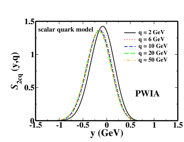
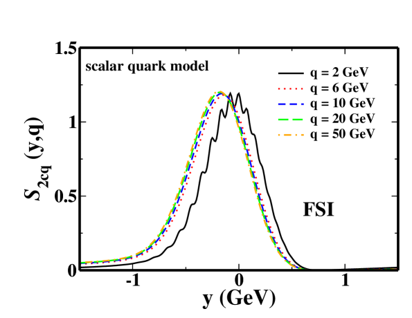
Figure 5: The scaling function ${\cal{S}}_{2cq}$ of the “scalar quark” model is plotted versus $y$ for several values of the three-momentum transfer $q$. The results shown in the top panel have been calculated in PWIA, i.e. for the bound-free transition. The results shown in the bottom panel have been calculated including final state interactions (FSI), i.e. for the bound-bound transition.

Now, we will proceed to show the $y$ scaling results for the ”scalar quark model” jvod2 , too. This will allow us to study the transition from a simple model to a more sophisticated version, and to point out differences and common features. In jvod2 , we included the proper spins for the beam electrons and the exchange photons, but still treated the quark as a scalar. We will refer to this model as the ”scalar quark model” in the present paper. This model has a conserved current, and a much richer structure, due to the fact that the photon can have transverse and longitudinal polarization, which leads to two structure functions. In Fig. 5, top panel, the PWIA results definitely scale more slowly than for the all scalar model. Scaling is reached at $q=20~{}GeV$. Not surprisingly, the FSI results, shown in the bottom panel of Fig. 5, exhibit an even slower scaling. Even from $q=20~{}GeV$ to $q=50~{}GeV$, a small difference is visible in the scaling curves. This is the slowest onset of $y$-scaling which we have encountered so far, and this mirrors precisely what we expected from our previous $u$-scaling results. Now we are in a good position to progress to the main topic of this paper, the results for proper spin-$1/2$ quarks. Our study of the onset of scaling for PWIA and FSI will allow us to draw some conclusions about the onset of $u$ scaling for the FSI case, even if we can’t calculate for the necessary $Q^{2}$ numerically. First, we are going to present results for the PWIA for three different potentials.

IV.3 y-scaling in PWIA

First, we show our results for PWIA, where we expect scaling to set in at lower momentum transfers than for the FSI results. For the FSI results, the scaling curve is generated in our model by many overlapping resonances, and one needs to reach kinematics where a sufficient number of resonances is accessible to see scaling.

The scaling variable y is defined by (20) and by inverting to find $\nu$ as a function of $y$ and $q$, the response functions can be written as functions of $q$ and $y$. For example the PWIA response functions (18) and (19) can be rewritten as

$$R_{L}(q,y) = \frac{1}{16\pi^{2}q}\int_{|y|}^{y+2q}dpp\biggl{\{}\sqrt{(y+q)^{2}+m^{2}}n^{0}_{v}(p)+m\,n_{s}(p)$$ (21)

$$\left.+\frac{y^{2}+2qy+p^{2}}{2p}\,n^{s}_{v}(p)\right\}$$

and

$$R_{T}(q,y) = \frac{1}{8\pi^{2}q}\int_{|y|}^{y+2q}dpp\biggl{\{}\sqrt{(y+q)^{2}+m^{2}}n^{0}_{v}(p)-m\,n_{s}(p)$$ (22)

$$\left.-\frac{y^{2}+2qy+2q^{2}-p^{2}}{2q}\,\frac{y^{2}+2qy-p^{2}}{2pq}\,n^{s}_{v}(p)\right\}\,.$$

In the limit of large $q$ the PWIA response functions become

$$\lim_{q\rightarrow\infty}R_{L}(q,y) = \frac{1}{16\pi^{2}}\int_{|y|}^{\infty}dpp\left\{n^{0}_{v}(p)+\frac{y}{p}\,n^{s}_{v}(p)\right\}$$ (23)

and

$$\lim_{q\rightarrow\infty}R_{T}(q,y) = \frac{1}{8\pi^{2}}\int_{|y|}^{\infty}dpp\left\{n^{0}_{v}(p)-\frac{y}{p}\,n^{s}_{v}(p)\right\}\,.$$ (24)

These response functions therefore scale in $y$. Note that the longitudinal response is shifted toward positive $y$ while the transverse is shifted toward negative $y$, since $n_{v}^{s}(p)$ is positive. The overall peak heights of the longitudinal and transverse responses in PWIA have roughly a $1:2$ ratio.

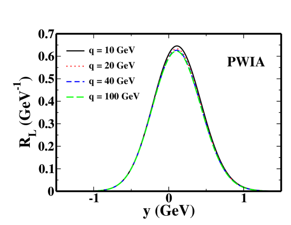
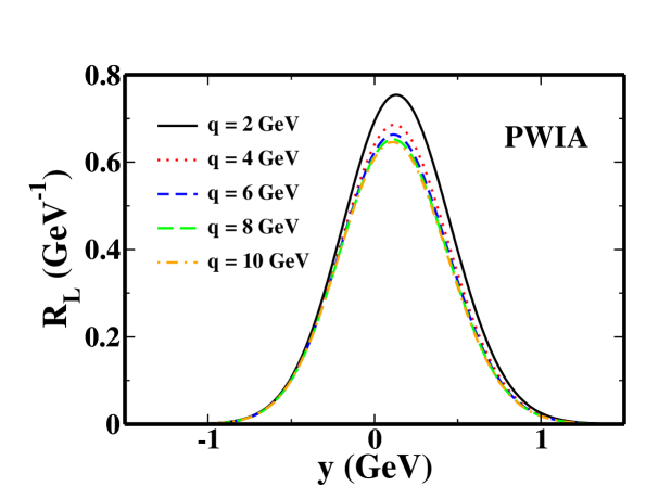
Figure 6: The longitudinal response function $R_{L}$ is plotted versus $y$ for several low (bottom panel) and high (top panel) values of the three-momentum transfer $q$. The results shown have been calculated in PWIA, using the linear potential.

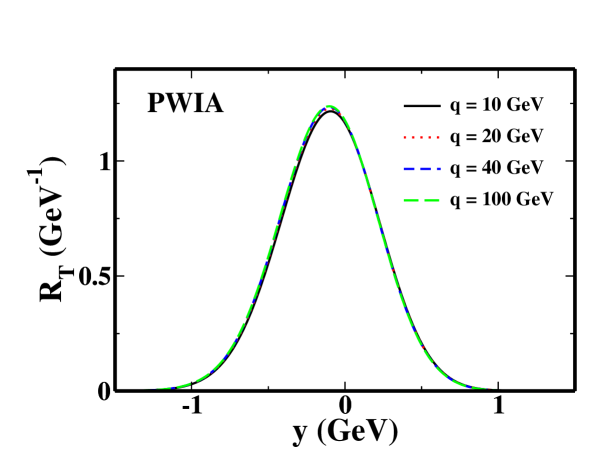
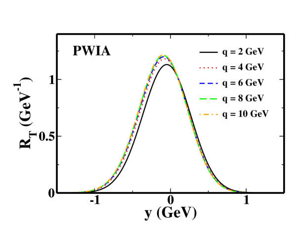
Figure 7: The transverse response function $R_{T}$ is plotted versus $y$ for several low (bottom panel) and high (top panel) values of the three-momentum transfer $q$. The results shown have been calculated in PWIA, using the linear potential.

We start by investigating the behavior of the PWIA responses for the linear potential: $V_{s}=br,V_{v}=0$. In Fig. 6, bottom panel, we show the longitudinal response $R_{L}$ for various, lower three-momentum transfers $q$. Here, one sees clearly that both the peak height and the width of the peak are reduced significantly by increasing $q$ for $q<10~{}GeV$. The peak position also shifts very slightly to lower $y$ values. In Fig. 6, top panel, we show the longitudinal response $R_{L}$ for various, high three-momentum transfers $q$. There is a small but visible change in going from $q=10~{}GeV$ to $q=20~{}GeV$. Scaling is reached for $q=40~{}GeV$, and the curves corresponding to even higher momentum transfers coincide.

In Fig. 7, we show the corresponding results for the transverse response function $R_{T}$. For the low momentum transfers, bottom panel, one sees that increasing $q$ leads to an increase in peak height and width, along with a small shift of the peak position towards lower $y$ values. The top panel with the high momentum transfers shows that scaling sets in faster for $R_{T}$ than for $R_{L}$. Changes are smaller from one $q$ value to the next, and the curves coincide once $q=40~{}GeV$.

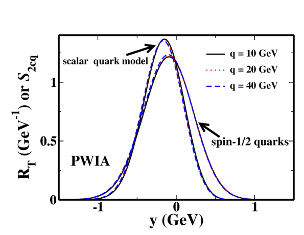
Figure 8: A comparison of the onset of scaling for the “scalar quark” model and the model with quark spin. The transverse response function $R_{T}$ and the scaling function ${\cal{S}}_{2cq}$ of the “scalar quark” model are plotted versus $y$. The results shown have been calculated in PWIA, and have already been shown in Figs. 7,5.

It is interesting to consider the onset of scaling when making our modeling more realistic: in the transition from the “all scalar” to the “scalar quark” model, we observed a considerable slowdown in the onset of scaling, due to the additional structure, and to the more complicated form of the terms. Now, we have added the proper spin to the quarks, but interestingly, we see no significant change in the scaling behavior. This is illustrated in Fig. 8, where we show high $q$ results for the scalar quark model and our current model. While the two models obviously lead to different scaling curves, the onset of scaling occurs at roughly the same momentum transfers in both cases. From this, we have to conclude that the spin of the quark does not play a significant role in the onset of scaling.

IV.4 y-scaling in FSI

Now we will show the scaling behavior with FSI included. For reasons of numerical feasibility, we restrict ourselves to momentum transfers of $q\leq 10~{}GeV$.

Figure 9 shows the longitudinal (top panel) and transverse responses (bottom panel) as a function of $y$ for momentum transfers from $2$ to $10$ GeV with a width of $\epsilon=0.02$ GeV for smoothing (recall Eq. (11)).

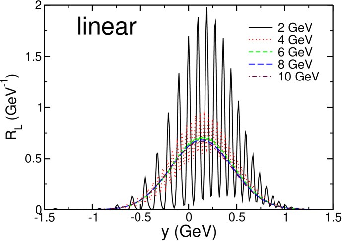
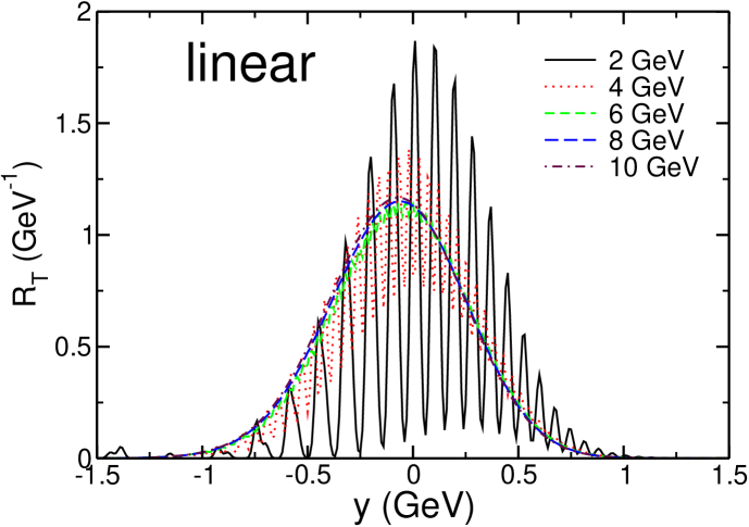
Figure 9: The longitudinal response function $R_{L}$ (top panel) and the transverse response function $R_{T}$ are plotted versus $y$ for several values of the three-momentum transfer $q$. The results shown have been calculated including FSI, using the linear potential.

As the momentum transfer increases, the average response moves to lower $y$ and since the density of states is also increasing the curves become increasingly smooth. The longitudinal response approaches the asymptotic result from above, while the transverse response approaches it from below. The low $q$ curves with the visible resonance bumps oscillate around the smoother curves obtained for higher momentum transfer.

Before comparing the scaling curves obtained in PWIA and with FSI, we need to investigate the influence of our smoothing procedure for the delta-function in energy. This is an artifact of our model, as we assume that the resonances do not decay. In jvod2 , we used a Breit-Wigner type smoothing procedure, and the width $\Gamma$ had some influence on the numerically obtained scaling curves. However, for the scalar quarks discussed in jvod2 , we could find an analytic expression for the scaling curve with FSI. This is not the case here, so this matter deserves careful investigation. The PWIA calculation does not suffer from this problem, as the knocked-out, “free” quark can have any energy, in contrast to the fixed-energy resonance final states included in FSI. Therefore, comparing the FSI and PWIA scaling curves is not entirely straightforward.

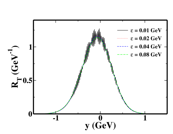
Figure 10: The transverse response calculated for the linear potential in FSI at $q=10~{}GeV$ for various values of the Gaussian smoothing parameter $\varepsilon$.

In Fig. 10, we show the transverse response $R_{T}$ at $q=10~{}GeV$, including FSI, calculated for various values of the Gaussian smoothing parameter $\varepsilon$. We show curves for $\varepsilon=0.02~{}GeV$, the value used for all other plots in this paper, and for $\varepsilon=0.01,0.04,0.08~{}GeV$. While a smaller value of $\varepsilon$ leads to less smoothing and visible resonance bumps even at higher $q$, the overall shape, peak position and width are not changed. For larger values of $\varepsilon$, there is no visible difference to the original curve with $\varepsilon=0.02~{}GeV$ . Therefore, the dependence on the smoothing parameter $\varepsilon$ is so weak that it will not influence our comparison of the PWIA and FSI scaling curves.

IV.5 Model dependence

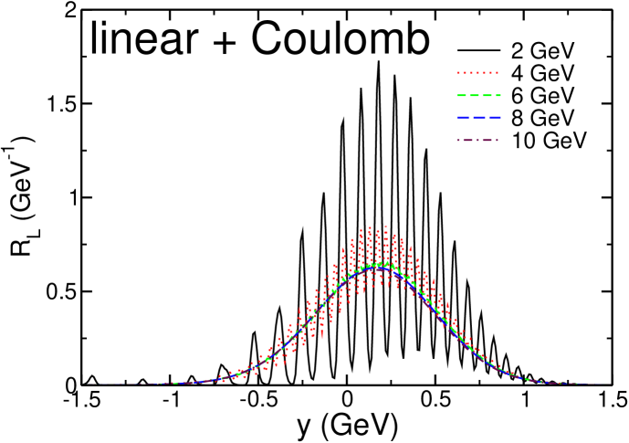
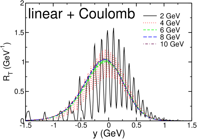
Figure 11: The longitudinal response function $R_{L}$ (top panel) and the transverse response function $R_{T}$ are plotted versus $y$ for several values of the three-momentum transfer $q$. The results shown have been calculated including FSI, using the linear-plus-Coulomb potential.

Calculations for the linear-plus-coulomb potential are shown in Fig. 11, and for the linear-plus-running potential in Fig. 12. These figures show features consistent with those of the linear potential alone. One can see that the linear potential leads to the highest peak value for both $R_{T}$ and $R_{L}$, and has the narrowest width, while the linear-plus-running potential has the lowest peak height and the largest width. In all cases, we have not quite reached the scaling limit yet, but as the changes from $q=6~{}GeV$ to $q=10~{}GeV$ are small, we are not far away from it, either. The low $q$ results clearly oscillate around the high $q$ results, as expected from duality.

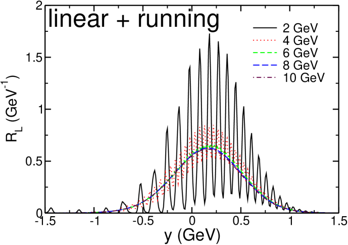
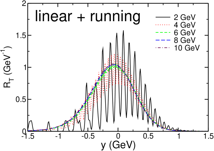
Figure 12: The longitudinal response function $R_{L}$ (top panel) and the transverse response function $R_{T}$ are plotted versus $y$ for several values of the three-momentum transfer $q$. The results shown have been calculated including FSI, using the linear-plus-running potential.

Figure 13 shows a comparison of the FSI and PWIA calculations at $q=10$ GeV for the longitudinal and transverse responses. At this momentum transfer the corresponding FSI and PWIA calculations differ by small changes in magnitude and peak position. Since the calculations are not yet converged to the scaling limit, it is not clear whether this represents a failure to scale to the same limit or is simply a manifestation of differing rates of convergence.

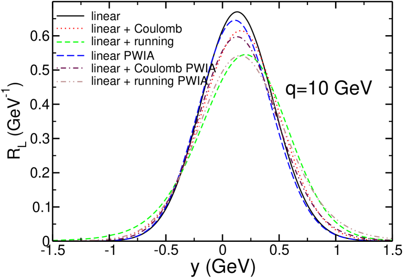
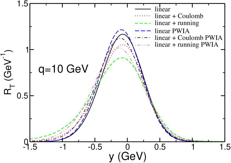
Figure 13:

On a fundamental level, this is important as FSI is usually assumed to be negligible in the analysis of deep inelastic scattering data. Recently, however, some authors have pointed out that FSI - through gluon exchange between fast, outgoing partons and target spectators - can make contributions to the leading twist structure functions at small $x_{Bj}$ hoyer . Still, the changes we see here are small, and one does not make much of a mistake in neglecting the effect of all the FSIs combined.

V Sum Rules

Some of the features of this model can be explored further and more precisely by means of energy-weighted sum rules. This will allow us to get a better feeling for the bulk features of our results, like peak position and width. Moments that become constant at high momentum transfer are another signature of quark-hadron duality prdmom , and with the sum rules derived in this section we can test if our model behaves in this way.

By using an integral representation of the energy conserving delta function and replacing eigenenergies with the hamiltonian operator, the response functions can be written as

$$R_{L}(q,\nu) = \int_{-\infty}^{\infty}\frac{dt}{2\pi}e^{i\nu t}<\Psi_{0}|e^{iH(\hat{\bm{p}},\bm{x})t}e^{-i\bm{q}\cdot\bm{x}}e^{-iH(\hat{\bm{p}},\bm{x})t}e^{i\bm{q}\cdot\bm{x}}|\Psi_{0}>$$ (25)

$$= \int_{-\infty}^{\infty}\frac{dt}{2\pi}e^{i\nu t}<\Psi_{0}|e^{i\hat{H}(\hat{\bm{p}},\bm{x})t}e^{-iH(\hat{\bm{p}}+\bm{q},\bm{x})t}|\Psi_{0}>$$

and

$$R_{T}(q,\nu) = \sum^{2}_{i=1}\int_{-\infty}^{\infty}\frac{dt}{2\pi}e^{i\nu t}<\Psi_{0}|e^{iH(\hat{\bm{p}},\bm{x})t}\alpha_{i}e^{-i\bm{q}\cdot\bm{x}}e^{-iH(\hat{\bm{p}},\bm{x})t}e^{i\bm{q}\cdot\bm{x}}\alpha_{i}|\Psi_{0}>$$ (26)

$$= \sum^{2}_{i=1}\int_{-\infty}^{\infty}\frac{dt}{2\pi}e^{i\nu t}<\Psi_{0}|e^{i\hat{H}(\hat{\bm{p}},\bm{x})t}\alpha_{i}e^{-iH(\hat{\bm{p}}+\bm{q},\bm{x})t}\alpha_{i}|\Psi_{0}>\,,$$

where the momentum shift operator has been recognized and used in the last step for both response functions.

The energy weighted sum rules are defined as integrals of the response functions over $-\infty<\nu<\infty$ weighted with powers of $\nu$. This integral can be simplified by writing

$$\nu^{n}e^{i\nu t}=\left(-i\frac{\partial}{\partial t}\right)^{n}e^{i\nu t}$$ (27)

and then integrating by parts to give

$${\cal S}_{Ln}(q) = \int_{-\infty}^{\infty}d\nu\,\nu^{n}R_{L}(q,\nu)$$ (28)

$$= \left(i\frac{\partial}{\partial t}\right)^{n}<\Psi_{0}|e^{iH(\hat{\bm{p}},\bm{x})t}e^{-iH(\hat{\bm{p}}+\bm{q},\bm{x})t}|\Psi_{0}>_{t=0}$$

and

$${\cal S}_{Tn}(q) = \int_{-\infty}^{\infty}d\nu\,\nu^{n}R_{T}(q,\nu)$$ (29)

$$= \sum^{2}_{i=1}\left(i\frac{\partial}{\partial t}\right)^{n}<\Psi_{0}|e^{iH(\hat{\bm{p}},\bm{x})t}\alpha_{i}e^{-iH(\hat{\bm{p}}+\bm{q},\bm{x})t}\alpha_{i}|\Psi_{0}>_{t=0}\,.$$

The momentum-shifted hamiltonian for our model is

$$H(\hat{\bm{p}}+\bm{q},\bm{x})=\bm{\alpha}\cdot\bm{q}+H(\hat{\bm{p}},\bm{x})\,.$$ (30)

As a result, the sum rules can be reduced to nested commutators involving $H$, $\bm{\alpha}\cdot\bm{q}$ and $\alpha_{i}$.

The first three sum rules for the longitudinal response are

$${\cal S}_{L0}(q) = <\psi_{0}|\psi_{0}>=1$$

$${\cal S}_{L1}(q) = <\psi_{0}|\bm{\alpha}\cdot\bm{q}|\psi_{0}>=0$$

$${\cal S}_{L2}(q) = q^{2}$$ (31)

The first of these is the Coulomb sum rule and simply reflects the conservation of charge. We have assumed that the charge of the bound quark is 1 for simplicity. The second of these indicates that the response is roughly antisymmetric about $\nu=0$. The third indicates that the width of the distribution is increasing as $q$. This is consistent with the case where the longitudinal response consists of peaks at positive and negative energy transfers of roughly equal magnitude and opposite signs that are moving away from the origin in opposite directions by a distance proportional to $q$. The existence of the negative energy peak is a consequence of the presence of the negative energy solutions to the Dirac equation which are not physical in a simple one-body model.

The positive energy contribution can be isolated by defining the positive energy moments

$$S_{L(T)n}(q)=\int_{0}^{\infty}d\nu\,\nu^{n}R_{L(T)}(\bm{q},\nu)\,.$$ (32)

Since the $n=0$ moment is no longer normalized to one, we can define the average energy transfer as

$$\left<\nu\right>_{L(T)}=\frac{S_{L(T)1}}{S_{L(T)0}}$$ (33)

and the rms variation in energy transfer as

$$\Delta\nu_{L(T)}=\sqrt{\frac{S_{L(T)2}}{S_{L(T)0}}-\left<\nu\right>_{L(T)}^{2}}\,.$$ (34)

Figures 14 and 15 show the positive energy $n=0$ moments of the longitudinal and transverse response functions. For $S_{L0}$, the results for the linear, linear-plus-coulomb, and linear-plus-running potentials are virtually identical except at $q>10\ {\rm GeV}$ where the moment starts to fall off due to finite range of excitation energies that have been calculated. The corresponding calculations in PWIA vary at small $q$ due to variations in the available phase space, but must approach $\frac{1}{2}$ for $q\rightarrow\infty$. It is clear from this figure that neither the FSI calculations nor the PWIA calculations have reached their saturation values at the highest values of $q$ that have been calculated here. Although it is plausible that the full results may be approaching the PWIA values for large $q$, it is not possible to determine that this is the case based on these calculations.

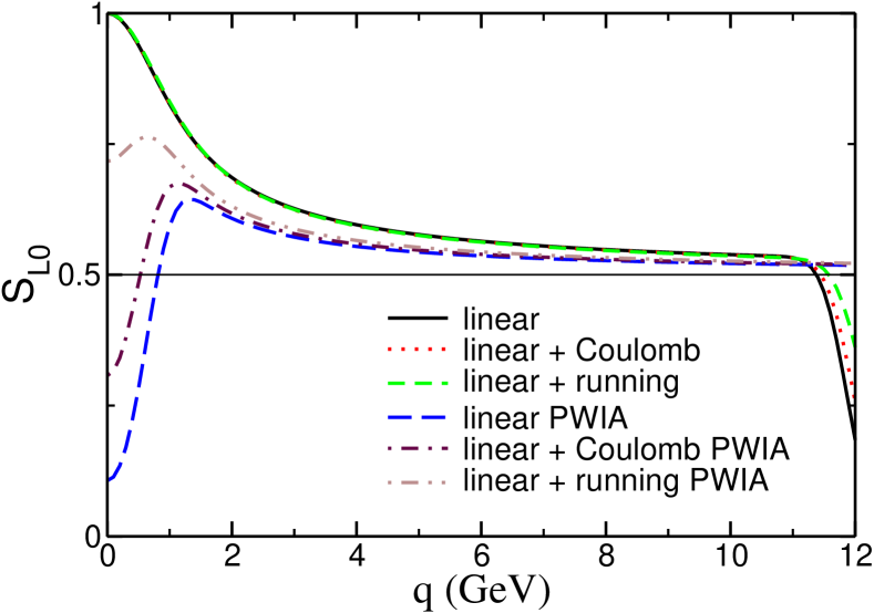
Figure 14: The positive energy $n=0$ moment of the longitudinal response function, calculated with FSI and in PWIA for the linear, linear-plus-coulomb, and linear-plus-running potentials.

Similar results can be seen for the transverse moment shown in Fig. 15 although there is a greater variation among the full calculations at lower values of $q$. In this case the asymptotic value of the moment for the PWIA calculations is 1.

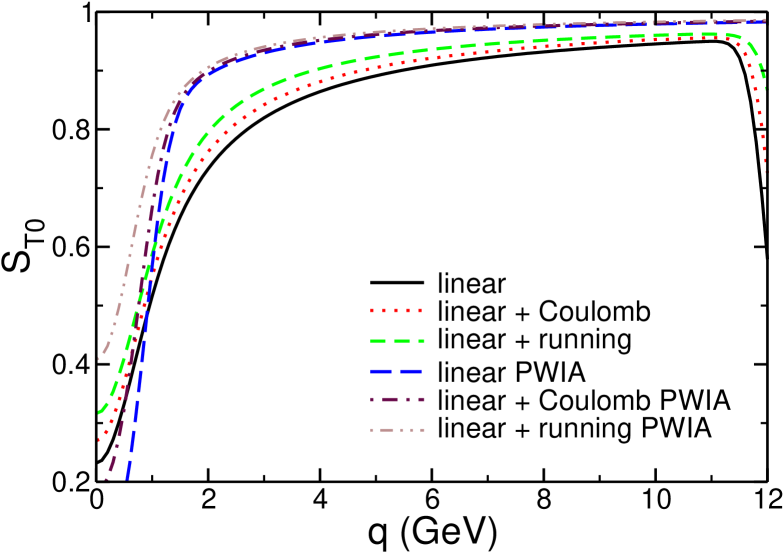
Figure 15: The positive energy $n=0$ moment of the transverse response function, calculated with FSI and in PWIA for the linear, linear-plus-coulomb, and linear-plus-running potentials.

The asymptotic values of $\left<\nu\right>_{L(T)}$ for the PWIA are given by

$$\lim_{q\rightarrow\infty}\left<\nu\right>_{L}=q-E_{0}+\frac{1}{12\pi^{2}}\int_{0}^{\infty}dp\,p^{3}n_{v}^{s}(p)$$ (35)

and

$$\lim_{q\rightarrow\infty}\left<\nu\right>_{T}=q-E_{0}-\frac{1}{12\pi^{2}}\int_{0}^{\infty}dp\,p^{3}n_{v}^{s}(p)\,.$$ (36)

Note that the longitudinal and transverse responses are offset from one another by terms that depend upon $n_{v}^{s}(p)$. Since the average value of the energy transfer increases linearly with $q$, it is convenient to plot this moment as $q-\left<\nu\right>_{L}$. This quantity is shown in Fig. 16 for the three FSI and three PWIA calculations used in the previous figures. Here the three FSI calculations have very similar average positions while the average positions of the PWIA calculations show large differences. This is the result of the sensitivity of the position of the peak of the PWIA response to the difference in energy of the bound state and the lowest plane-wave state. In the FSI calculation, both the ground and excited states see the same potential which seems to limit the size of the shift in peak position for the three different potentials.

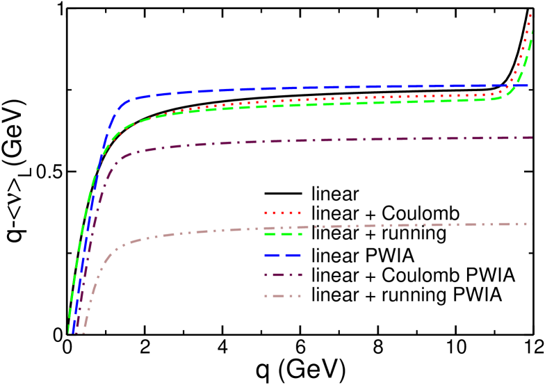
Figure 16: The difference $q-\left<\nu\right>_{L}$ between the average energy transfer $\left<\nu\right>_{L}$ and the momentum transfer for the longitudinal response, calculated with FSI and in PWIA for the linear, linear-plus-coulomb, and linear-plus-running potentials.

For purposes of comparison, it is possible to eliminate this disparity in the PWIA calculations by introducing a constant vector potential into the Dirac equation. This has the effect of simply shifting the spectrum. As a result we can use this shift to place all of the ground state energies at the same value. This shift has no effect on the response functions for the FSI calculations, but will correct for the differences in phase space in the PWIA. In fact, we already have applied this shift above in the section on y-scaling.

Figure 17 shows the rms widths for the various calculations of the longitudinal response. The asymptotic value of this width in the PWIA is given by

$$\lim_{q\rightarrow\infty}\Delta\nu_{L}=\left[\frac{1}{12\pi^{2}}\int_{0}^{\infty}dp\,p^{4}n_{v}^{0}(p)-\frac{1}{144\pi^{4}}\left(\int_{0}^{\infty}dp\,p^{3}n_{v}^{s}(p)\right)^{2}\right]^{\frac{1}{2}}\,.$$ (37)

In all three cases the width of the FSI calculation is close to that of the corresponding PWIA calculation. This suggests that the width of the response is determined largely by the width of ground state momentum distributions.

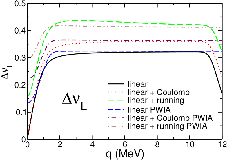
Figure 17: The rms width $\Delta\nu_{L}$ for the longitudinal response, calculated with FSI and in PWIA for the linear, linear-plus-coulomb, and linear-plus-running potentials.

While we have not yet reached convergence to the scaling limit at the momentum transfers for which we have calculated, one can clearly see that the moments do flatten out with higher momentum transfers, qualitatively agreeing with the observations in duality experiments.

VI The “y-scaling Callan-Gross relation”

From $x$-scaling in the deep inelastic region, the Callan-Gross relation callangross $2xF_{1}(x)=F_{2}(x)$ is known to hold. The physical significance of the Callan-Gross relation is that one scatters off spin $1/2$ objects, which have a dominant contribution from the magnetization current, i.e. in the transverse part of the structure functions. In the real world, the Callan-Gross relation needs to be corrected for radiative effects, and is then observed to hold in the experimental data from the deep inelastic region. In our model, there are no radiative corrections, as we do not allow the production of new particles. Our model is, so far, entirely quantum-mechanical in this sense. Therefore, we expect the Callan-Gross relation to hold as is in $x$ or $u$ scaling. As we focus on $y$ scaling, we now derive the analog of the Callan-Gross relation, using the fact that both the longitudinal and the transverse response scale for large $q$.

The structure functions $W_{1},W_{2}$ are related to the longitudinal and transverse responses $R_{L}$ and $R_{T}$ by

$$W_{1}=\frac{1}{2}R_{T}$$ (38)

and

$$W_{2}=\frac{Q^{4}}{q^{4}}R_{L}+\frac{Q^{2}}{2q^{2}}R_{T}\,$$ (39)

The Callan-Gross relation can be obtained from these equations by re-expressing $q$ and $\nu$ in terms of $x$ and $Q^{2}$, and increasing $Q^{2}$ at fixed $x$. In order to find an analogous relation for $y$ scaling, we re-express $Q^{2}$ and $\nu$ in terms of $q$ and $y$, and then increase $q$ at fixed $y$. The kinematic factors in this limit become

$$\nu\frac{Q^{2}}{2q^{2}}\to E_{0}-y$$ (40)

and

$$\frac{Q^{4}}{q^{4}}\to O\left(\frac{1}{q^{2}}\right)\to 0\,.$$ (41)

The two functions, $F_{1}=MW_{1}$ and $F_{2}=\nu W_{2}$, in this limit are:

$$F_{1}=MW_{1}=\frac{1}{2}MR_{T}\to\frac{1}{2}MR_{T}$$ (42)

$$F_{2}=\nu W_{2}=\nu\frac{Q^{4}}{q^{4}}R_{L}+\nu\frac{Q^{2}}{2q^{2}}R_{T}\to(E_{0}-y)R_{T}$$ (43)

Direct comparison of Eqs. (42) and (43) yields $F_{2}=F_{1}\frac{2}{M}(E_{0}-y)$. Substituting the definitions of $F_{1}$ and $F_{2}$, one obtains the analog of the Callan-Gross relation for $y$-scaling:

$$2W_{1}(E_{0}-y)=\nu W_{2}\,.$$ (44)

We now proceed to check if our numerical results fulfill the Callan-Gross relation, i.e. if we have reached the scaling region already. First, we show results for PWIA, where we can access arbitrarily high $q$ without any numerical problems. In order to display the approach to scaling, we show the ratio of the left-hand-side to the right-hand-side of Eq. (44), $r_{CG}=2W_{1}(E_{0}-y)/\nu W_{2}$. In Fig. 18, top panel, we show $r_{CG}$ for the linear potential for values of the three momentum ranging from $q=10~{}GeV$ to $q=1000~{}GeV$. As expected, scaling has set in at these high momentum transfers: the deviations of $r_{CG}$ from $1$ are very small, at the level of $5\%$ or less for $q\geq 60~{}GeV$. It is interesting to note that for higher $y$ values, $\nu W_{2}$ dominates, while for lower $y$ values, $2W_{1}(E_{0}-y)$ is larger. As in the calculation of the response functions, we have applied the energy shift to adjust the difference in phase space in PWIA. Note that we have omitted the regions $y<-1GeV$ and $y>0.7GeV$ from our graphs, as they do not contain any strength in the responses. The latter is the area where $(E_{0}-y)$ undergoes a sign change, leading to a spike in the ratio $r_{CG}$ that is unrelated to the interesting physics - there is hardly any strength in the responses for $y>0.5~{}GeV$.

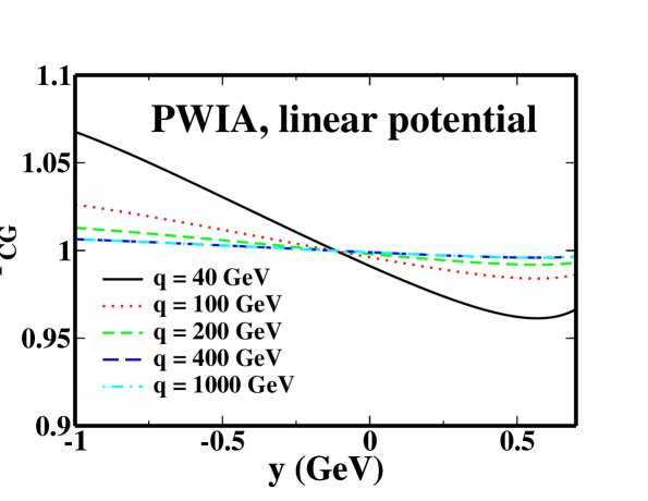
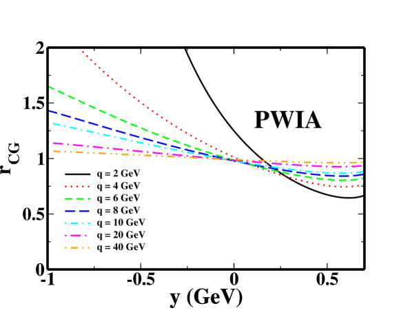
Figure 18: The Callan-Gross ratio $r_{CG}$ is plotted versus $y$ for several values of the three-momentum transfer $q$. The results shown have been calculated in PWIA with a linear potential. Note the different scales employed in the two panels.

For lower $q$ values, see bottom panel of Fig. 18, scaling has clearly not yet set in, and the deviations of $r_{CG}$ from unity are large. Comparing these results for $r_{CG}$ with the onset of scaling observed in the PWIA response functions $R_{L}$ and $R_{T}$, as discussed in Section IV.3, we see that $r_{CG}$ gives additional information on the scaling behavior. While the response function plots show that the curves coincide for $q=40~{}GeV$, at the latest, the Callan-Gross ratio is more sensitive and still shows slight changes for increasing three-momentum transfers.

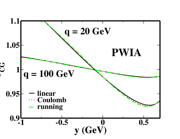
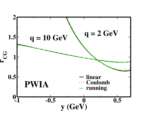
Figure 19: The Callan-Gross ratio $r_{CG}$ is plotted versus $y$ for the linear, Coulomb and running potential, for three-momentum transfers $q=2,10,20,and100GeV$. The results shown have been calculated in PWIA. Note the different scales employed in the two panels.

Comparing the approach of $r_{CG}$ to $1$ for different potentials, Fig. 19 shows that linear, Coulomb, and running potentials have an almost identical scaling behavior, both at low and high $q$ values.

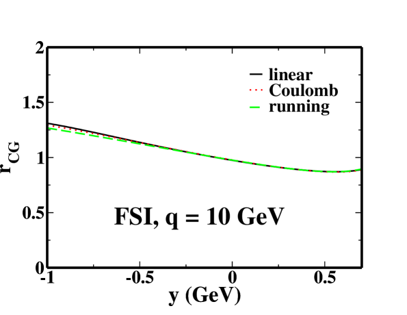
Figure 20: The Callan-Gross ratio $r_{CG}$ is plotted versus $y$ for three-momentum transfer $q=10~{}GeV$. The results shown have been calculated in FSI with a linear, Coulomb, and running potential.

In Fig. 20, we show $r_{CG}$ calculated including FSI for $q=10~{}GeV$, the highest value we have attained for FSI calculations. The calculations shown are performed for the different potentials considered in this paper, and one can see that, just like for PWIA, the results for the Callan-Gross ratio $r_{CG}$ are very similar.

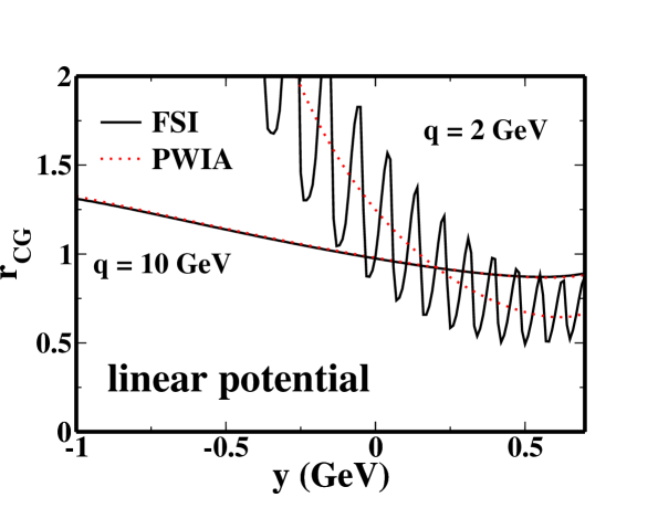
Figure 21: The Callan-Gross ratio $r_{CG}$ is plotted versus $y$ for three-momentum transfers $q=2~{}GeV$ and $q=10~{}GeV$. The results shown have been calculated in PWIA and FSI with a linear potential.

This similarity to the behavior of the PWIA curves leads us to a direct comparison of the PWIA and FSI results for the linear potential in Fig. 21. The PWIA and FSI agree very nicely. For lower $q$ values, the FSI results obviously lead to oscillatory behavior, but they average to the smooth PWIA result. The PWIA and FSI results for the Coulomb potential also track each other very closely. For the running potential, the differences between FSI and PWIA are a bit more visible, but FSI and PWIA results are still very close.

While this is no proof, this behavior leads one to the conjecture that scaling for FSI should set in at the same $q$ value as for PWIA, and that the rate of convergence in both cases is the same. Note that this result does not imply that the individual scaling results for PWIA and FSI are the same. Quite on the contrary, as we found that the FSI results at $q=10~{}GeV$ are not that close to the PWIA scaling curve, and as the PWIA results did not change dramatically from $q=10~{}GeV$ to higher $q$ values, the conjecture of the same rate of convergence suggests that the final scaling results in PWIA and FSI might be different.

VII Summary and Outlook

In the present paper, we have expanded our modeling of quark-hadron duality to describe a more realistic situation: we now include the spin of the quark. Numerically, this is more complicated than the all scalar model ijmvo and the scalar quark model jvod2 , where the solutions could be found analytically. However, the inclusion of the quark spin paves the way to study spin structure functions, which are one of the most promising areas for the practical application of quark-hadron duality.

We have tracked the changes introduced by making our models more realistic. Most notably, adding spin to the quark does not seem to influence the onset of scaling: our present model shows about the same scaling behavior as the scalar quark model. This is in contrast to the major changes in scaling behavior observed when going from the all scalar model to the scalar quark model.

As before, we have seen that the features of duality observed in experiments, namely scaling, oscillation of the resonances around the scaling curve, and flat moments at higher momentum transfer, are reproduced qualitatively. We have used a constituent quark mass of $m=258.46~{}MeV$ for our calculations. This number was taken from a fit to heavy mesons waw . However, nothing hinges on using that particular value: we changed our quark mass to $m=10~{}MeV$, in order to have a value reminiscent of a current quark mass, and repeated our calculations. It turns out that, while scaling does set in a little faster, there are no qualitative changes in the results.

In spite of the considerable numerical effort, we have not yet reached full convergence in FSI. Therefore, the important question if the FSI scaling curve coincides with the PWIA scaling curve could not be answered with certainty yet. At the highest $q$ value we reached, $q=10~{}GeV$, we still see small differences between FSI and PWIA curves. Further investigation of the high $q$ region with different methods will be the subject of a future paper.

Our findings are different from the results in mpdirac . There, the author used massless quarks and a specific assumption about the potential, namely an identical functional form for the scalar potential $V_{s}$ and the vector potential $V_{v}$. The condition $V_{s}=V_{v}$ leads to a simplification in the numerics, as upper and lower components decouple. Results reported in mpdirac indicate a much larger difference between FSI and PWIA results at $q=10~{}GeV$. This may be due to the potential chosen there.

For the first time, we have discussed several different potentials. The combination of a scalar linear potential and a vector color Coulomb potential (either with a running coupling constant or without) can be considered a fairly realistic approximation to nature. We were also able to demonstrate that the observed qualitative features of duality- scaling, low $q$ duality, convergence of the moments - persist no matter which potential is used. This hints at quark-hadron duality as a fairly general property of inclusive electron scattering. While the shape of the response functions is clearly influenced by the ground state momentum distribution, and therefore by the potential, the rate of convergence to scaling is unaffected by the choice of potential, as demonstrated by studying the validity of the y-scaling Callan-Gross relation.

Duality has been thoroughly explored experimentally in the unpolarized nucleon structure functions, and new data on polarization observables are available, too, both from Jefferson Lab jlabspin and Hermes at DESY hermes . We will apply our model to the calculation of spin structure functions next.

Acknowledgments: S.J. thanks the Theory Group of Jefferson Lab for their kind hospitality. This work was supported in part by funds provided by the U.S. Department of Energy (DOE) under cooperative research agreement under No. DE-AC05-84ER40150 and by the National Science Foundation under grant No. PHY-0139973.

References

- (1) E. D. Bloom and F. J. Gilman, Phys. Rev. Lett. 25, 1140 (1970); Phys. Rev. D 4, 2901 (1971).
- (2) I. Niculescu et al., Phys. Rev. Lett. 85, 1182 (2000); Phys. Rev. Lett. 85, 1186 (2000); R. Ent, C.E. Keppel and I. Niculescu, Phys. Rev. D 62, 073008 (2000); S. Liuti, R. Ent, C. E. Keppel and I. Niculescu, Phys. Rev. Lett. 89, 162001 (2002); J. Arrington, R. Ent, C. E. Keppel, J. Mammei and I. Niculescu, arXiv:nucl-ex/0307012.
- (3) C. S. Armstrong, R. Ent, C. E. Keppel, S. Liuti, G. Niculescu and I. Niculescu, Phys. Rev. D 63, 094008 (2001)
- (4) F. E. Close and N. Isgur, Phys. Lett. B 509, 81 (2001).
- (5) F. E. Close and Q. Zhao, 66, 054001 (2002); Q. Zhao and F. E. Close, Phys. Rev. Lett. 91, 022004 (2003).
- (6) F. E. Close and W. Melnitchouk, Phys. Rev. C 68, 035210 (2003) [arXiv:hep-ph/0302013].
- (7) M. W. Paris and V. R. Pandharipande, Phys. Lett. B 514, 361 (2001); M. W. Paris, Eur. Phys. J. A 17, 401 (2003); M. W. Paris and V. R. Pandharipande, Phys. Rev. C 65, 035203 (2002).
- (8) M. W. Paris, Phys. Rev. C 68, 025201 (2003).
- (9) V. R. Pandharipande, M. W. Paris and I. Sick, arXiv:nucl-th/0308078.
- (10) Y. B. Dong and J. He, Nucl. Phys. A 720, 174 (2003).
- (11) Y. B. Dong and M. F. Li, Phys. Rev. C 68, 015207 (2003).
- (12) A. Le Yaouanc, D. Melikhov, V. Morenas, L. Oliver, O. Pene and J. C. Raynal, Phys. Lett. B 488, 153 (2000).
- (13) R. Fiore, A. Flachi, L. L. Jenkovszky, A. I. Lengyel and V. K. Magas, Eur. Phys. J. A 15, 505 (2002) [arXiv:hep-ph/0206027]; L. Jenkovszky, V. K. Magas and E. Predazzi, Eur. Phys. J. A 12, 361 (2001) [arXiv:hep-ph/0110374].
- (14) G. Ricco, M. Anghinolfi, M. Ripani, S. Simula and M. Taiuti, Phys. Rev. C 57, 356 (1998); S. Simula, Phys. Lett. B 481, 14 (2000).
- (15) N. Isgur, S. Jeschonnek, W. Melnitchouk, and J. W. Van Orden, Phys. Rev. D 64, 054005 (2001).
- (16) S. Jeschonnek and J. W. Van Orden, Phys. Rev. D 65, 094038 (2002).
- (17) J. W. Van Orden and S. Jeschonnek, Eur. Phys. J. A17, 391 (2003).
- (18) “The Science Driving the 12 GeV Upgrade of CEBAF”, White Paper, Jefferson Lab 2001, edited by L. Cardman, R. Ent, N. Isgur, J.-M. Laget, C. Leemann, C. Meyer, Z.-E. Meziani.
- (19) M. A. Shifman, A. I. Vainshtein and V. I. Zakharov, Nucl. Phys. B 147, 448 (1979); M. A. Shifman, A. I. Vainshtein and V. I. Zakharov, Nucl. Phys. B 147, 385 (1979); A. I. Vainshtein, V. I. Zakharov, V. A. Novikov and M. A. Shifman, Sov. J. Nucl. Phys. 32, 840 (1980); E. C. Poggio, H. R. Quinn and S. Weinberg, Phys. Rev. D 13, 1958 (1976); A.V. Radyushkin, in Strong Interactions at Low and Intermediate Energies, ed. J.L. Goity (World Scientific, 2000), [hep-ph/0101227]; T. D. Cohen, R. J. Furnstahl, D. K. Griegel and X. Jin, Prog. Part. Nucl. Phys. 35, 221 (1995).
- (20) R. F. Lebed and N. G. Uraltsev, Phys. Rev. D 62, 094011 (2000).
- (21) See e.g. I. Bigi and N. Uraltsev, hep-ph/0106346;I. Bigi, M. Shifman, N. Uraltsev and A. Vainshtein, Phys. Rev. D 59, 054011 (1999); B. Grinstein and R. F. Lebed, Phys. Rev. D 59, 054022 (1999); B. Grinstein and R. F. Lebed, Phys. Rev. D 57, 1366 (1998); C. G. Boyd, B. Grinstein and A. V. Manohar, Phys. Rev. D 54, 2081 (1996).
- (22) N. Isgur and M. B. Wise, Phys. Rev. D 43, 819 (1991).
- (23) A.De Rújula, H. Georgi and H.D. Politzer, Annals Phys. 103, 315 (1977); Phys. Lett. B 64, 428 (1977).
- (24) X. Ji and P. Unrau, Phys. Rev. D 52, 72 (1995); X. Ji and P. Unrau, Phys. Lett. B 333, 228 (1994); X. Ji and W. Melnitchouk, Phys. Rev. D 56, 1 (1997).
- (25) N. Isgur, Phys. Rev. D 59, 034013 (1999).
- (26) Xiachao Zheng et al., submitted to Phys. Rev. Lett. arXiv:nucl-ex/0308011.
- (27) J. Zeng, J. W. Van Orden and W. Roberts, Phys. Rev. D 52, 5229 (1995).
- (28) S. Godfrey and N. Isgur, Phys. Rev. D 32, 189 (1985).
- (29) O.W. Greenberg, Phys. Rev. D 47, 331 (1993)
- (30) S.A. Gurvitz and A.S. Rinat, Phys. Rev. C 47, 2901 (1993); S.A. Gurvitz, Phys. Rev. D 52, 1433 (1995).
- (31) D. R. Harrington, Phys. Rev. C 66, 065205 (2002).
- (32) E. Pace, G. Salme and F.M. Lev, Phys. Rev. C 57, 2655 (1998).
- (33) S. J. Brodsky, P. Hoyer, N. Marchal, S. Peigne and F. Sannino, Phys. Rev. D 65, 114025 (2002) [arXiv:hep-ph/0104291].
- (34) C. G. Callan and D. Gross, Phys. Rev. Lett. 22, 156 (1969).
- (35) R. Fatemi et al. [CLAS Collaboration], arXiv:nucl-ex/0306019; Jefferson Lab Experiment E97-103, spokespersons T. Averett and W. Korsch.
- (36) A. Airapetian et al. [HERMES Collaboration], Phys. Rev. Lett. 90, 092002 (2003)