Study of $B\to D^{**}\pi$ decays

Abstract

We investigate the production of the novel $P$-wave mesons $D^{*}_{0}$ and $D^{\prime}_{1}\,(D_{1})$, identified as $J^{P}=0^{+}$ and $1^{+}$, in heavy $B$ meson decays, respectively. With the heavy quark limit, we give our modelling wave functions for the scalar meson $D^{*}_{0}$. Based on the assumptions of color transparency and factorization theorem, we estimate the branching ratios of $B\to D^{*}_{0}\pi$ decays in terms of the obtained wave functions. Some remarks on $D^{(\prime)}_{1}$ productions are also presented.

I Introduction

It is doubtless that quark model provides a successful method to describe the hadron spectroscopy. For instance, based on the SU(3) flavor symmetry, quark and anti-quark can comprise octet and singlet states, called nonet together, such as the well known pesudoscalar mesons of pion, kaon and eta with $J^{PC}=0^{-+}$. However, if we apply the same concept on the light scalar mesons described by $0^{++}$, such as the nonet composed of isoscalars $\sigma(600)$ and $f_{0}(980)$, isovector $a_{0}(980)$ and isodoublet $\kappa$, there are some puzzles (a) why $a_{0}(980)$ and $f_{0}(980)$ are degenerate in masses and (b) why the widths of $\sigma$ and $\kappa$ are broader than those of $a_{0}(980)$ and $f_{0}(980)$ Cheng . It is probable that these scalar states consist of four-quark rather than two-quark 4q . Moreover, the possibilities of $K\bar{K}$ molecular states, gluonium states and scalar glueballs are also proposed. It is clear that the conclusion is still uncertain.

Now, the mysterious event happens not only in the light scalar meson system, but also in the heavy $\bar{c}s$ one. Recently, BABAR collaboration has observed one narrow state, denoted by $D^{*}_{sJ}(2317)$, from a $D^{+}_{s}\pi^{0}$ mass distribution Babar1 . Furthermore, the same state has been confirmed by CLEO and a new state $D^{*}_{sJ}(2463)$ is also observed in the $D^{*+}_{s}\pi^{0}$ final state CLEO . Finally, BELLE verifies the observations Belle1 . By the data analysis, $D^{*}_{sJ}(2317)$ and $D^{*}_{sJ}(2463)$ are identified as parity-even states with ${\bf 0}^{+}$ and ${\bf 1}^{+}$, respectively. From the observations, the interesting problem is that the states of $D^{*}_{sJ}(2317)$ and $D^{*}_{sJ}(2463)$ cannot match with theoretical predictions Theory , i.e., the masses (widths) are too low (narrow). To explain the discrepancy, either the theoretical models have to be modified BEH or the observed states are the new composed states. To satisfy the latter, many interesting solutions have been suggested recently in Refs. CJ ; BCL ; BR ; YH ; Szczepaniak ; CD ; Chen-Li .

In fact, before the BABAR’s observation, CLEO CLEO-96 and BELLE Belle-conf measured the similar states in the $\bar{c}q$ ($q=u,d$) system in heavy $B$ meson decays. With two-quark picture, there are four parity-even (angular momentum $\ell=1$) states described by $J^{P}=0^{+}$, $1^{+}$, $1^{+}$ and $2^{+}$, respectively. $J=j_{q}+S_{Q}$ is the total angular momentum of the corresponding meson and consists of the angular momentum of the light quark, $j_{q}$, and the spin of the heavy quark, $S_{Q}$, where $j_{q}=S_{q}+\ell$ is combined by the spin and orbital angular momenta of the light quark. In the literature, they are usually labeled by $D^{*}_{0}$, $D^{\prime}_{1}$, $D_{1}$ and $D^{*}_{2}$, respectively. We also use $D^{**}$ to denote all of them. The first two belong to $j_{q}=1/2$, while the last two $j_{q}=3/2$. In the heavy quark limit, it is known that $D^{*(\prime)}_{0(1)}$ and $D^{(*)}_{1(2)}$ decay only via $S$ and $D$-wave, respectively. Therefore, one expects that the widths of the former are much broader than those of the latter, which is consistent with the observations of CLEO and BELLE CLEO-96 ; Belle-conf . Even the BELLE’s updated data Belle-new also show the same phenomenon. We now summarize the results of CLEO and BELLE as follows: in CLEO, the masses (widths) of $P$-wave states are given by $m_{D_{1}}(\Gamma_{D_{1}})=2422.0\pm 2.1\;(18.9^{+4.6}_{-3.5})$ and $m_{D^{*}_{2}}(\Gamma_{D^{*}_{2}})=2458.9\pm 2.0\;(23\pm 5)$ MeV, and the measured branching ratios (BRs) of $B$ decays are given as

$$BR(B^{-}\to D^{0}_{1}\pi^{-})\times BR(D^{0}_{1}\to D^{*+}\pi^{-})=(7.8\pm 1.9)\times 10^{-4},$$

$$BR(B^{-}\to D^{*0}_{2}\pi^{-})\times BR(D^{*0}_{2}\to D^{*+}\pi^{-})=(4.2\pm 1.7)\times 10^{-4}.$$ (1)

In BELLE, the four states are all measured as $m_{D^{*}_{0}}(\Gamma_{D^{*}_{0}})=2308\pm 17\pm 15\pm 28\;(276\pm 21\pm 18\pm 60)$, $m_{D^{\prime}_{1}}(\Gamma_{D^{\prime}_{1}})=2427.0\pm 26\pm 20\pm 15\;(384^{+107}_{-75}\pm 24\pm 70)$, $m_{D_{1}}(\Gamma_{D_{1}})=2421.4\pm 1.5\pm 0.4\pm 0.8\;(23.7\pm 2.7\pm 0.2\pm 4.0)$, and $m_{D^{*}_{2}}(\Gamma_{D^{*}_{2}})=2461.6\pm 2.1\pm 0.5\pm 3.3\;(45.6\pm 4.4\pm 6.5\pm 1.6)$ MeV, and the BRs with possible decaying chain being

$$BR(B^{-}\to D^{*0}_{0}\pi^{-})\times BR(D^{*0}_{0}\to D^{+}\pi^{-})=(6.1\pm 0.6\pm 0.9\pm 1.6)\times 10^{-4},$$

$$BR(B^{-}\to D^{{}^{\prime}0}_{1}\pi^{-})\times BR(D^{\prime 0}_{1}\to D^{*+}\pi^{-})=(5.0\pm 0.4\pm 1.0\pm 0.4)\times 10^{-4},$$

$$BR(B^{-}\to D^{0}_{1}\pi^{-})\times BR(D^{0}_{1}\to D^{*+}\pi^{-})=(6.8\pm 0.7\pm 1.3\pm 0.3)\times 10^{-4},$$

$$BR(B^{-}\to D^{*0}_{2}\pi^{-})\times BR(D^{*0}_{2}\to D^{+}\pi^{-})=(3.4\pm 0.3\pm 0.6\pm 0.4)\times 10^{-4},$$

$$BR(B^{-}\to D^{*0}_{2}\pi^{-})\times BR(D^{*0}_{2}\to D^{*+}\pi^{-})=(1.8\pm 0.3\pm 0.3\pm 0.2)\times 10^{-4},$$ (2)

respectively.

Since the masses of $D^{*}_{sJ}$ are just below the $D^{(*)}K$ threshold and the corresponding widths are around few $10$ KeV YH , both parity-even mesons could only decay through isospin violating channels to $D\pi$ and $D^{*}\pi$. Due to this reason, it becomes the main problem how to explain the low masses and narrow widths for $D^{*}_{sJ}$ states. Unlike $D^{*}_{sJ}$ cases, however, there are no any suppressions on their decays to $D\pi$ or $D^{*}\pi$ although the measured masses of $D^{**}$ are slightly different from the predictions of theoretical models. It is believed that the properties of $D^{**}$ could be described by current theoretical models with some improvements. If so, based on the concept of the normal quark model, we could further understand the nature of $D^{**}$ in $B$ decays.

To handle the hadronic effects for $B\to D^{**}\pi$ decays, we use the factorization formalism, called perturbative QCD (PQCD) approach, which is based on factorization theorem and the transition matrix element is described by the convolution of hadron wave functions and the hard kernel LB ; Li . The wave functions in principle can be extracted by experimental data or determined by QCD sum rules or lattice calculations. The hard kernel is related to the hard gluon exchange and high energetic fermion propagator, which are all calculable perturbatively. At the limit of heavy quark, in order to guarantee that color transparency mechanism Bjorken is satisfied, i.e., no soft gluon exchange between the final states, we need the hierarchy of $m_{B}>>m_{D^{**}}>>\bar{\Lambda}$ with $\bar{\Lambda}\sim m_{B}-m_{b}\sim m_{D^{**}}-m_{c}$ KLS . It has been shown by Ref. PQCD-Group that with the same QCD approach, the calculated results on $B\to D\pi$ decays are consistent with the current observations PDG . Consequently, one expects that PQCD could be also applied to the $P$-wave meson production in $B$ decaying processes. By the study, we should know more properties related to $P$-wave mesons.

The paper is organized as follows. We investigate the characteristic of $D^{**}$ and model their amplitude distributions in Sec. II. In terms of PQCD approach, we derive the factorization formulas for each $B\to D^{*}_{0}\pi$ decays in Sec. III. We present our results in Sec. IV. Finally, we give a summary in Sec. V.

II Decay constants and wave functions of $D^{**}$

In order to study the production of the scalar meson $D^{**}$ in $B$ decays, we immediately have to face two questions. The first one is how to write down the hadronic structures and model the wave functions of $D^{**}$, and the second is what the values of decay constants of $D^{**}$ are. In PQCD, since the wave functions belong to nonperturbative objects and are universal, we can directly apply the wave functions of $B$ and $\pi$ mesons, which have been discussed in other $B$-meson decays, such as $B\to\pi\ell\nu$, $B\to\pi\pi$ etc. Therefore, the hadronic structures of $B$ and $\pi$ mesons can be described by KLS-PRD ; Ball

$$\langle 0|\bar{b}(0)_{j}d(z)_{l}|B,p_{1}\rangle = \frac{1}{\sqrt{2N_{c}}}\int^{1}_{0}dxe^{-ixp_{1}\cdot z}\Big{\{}[/p_{1}+m_{B}]_{lj}\gamma_{5}\Phi_{B}(x)\Big{\}},$$

$$\langle 0|\bar{u}(0)_{j}d(z)_{l}|\pi,p_{3}\rangle = \frac{1}{\sqrt{2N_{c}}}\int^{1}_{0}dxe^{-ixp_{3}\cdot z}\Big{[}[/{p_{3}}]_{lj}\Phi_{\pi}(x)$$ (3)

$$+m^{0}_{\pi}[I]_{lj}\Phi_{\pi}^{p}(x)+m^{0}_{\pi}[/{n_{-}}/{n_{+}}-I]_{lj}\Phi^{\sigma}_{\pi}(x)\Big{]},$$

where $n_{-}=(0,1,\vec{0}_{T})$, $n_{+}=(1,0,\vec{0}_{T})$ and $x$ is the momentum fraction of the light parton inside the corresponding meson. $\Phi_{\pi}$ and $\Phi^{p(\sigma)}_{\pi}$ are the twist-2 and twist-3 pion wave functions, related to the distribution amplitude of nonlocal operator $\bar{u}\gamma_{5}\gamma_{\mu}d(z)$ and associated with $\bar{u}\gamma_{5}d(z)$ ($\bar{u}\gamma_{5}\sigma_{\mu\nu}d(z)$), respectively. We note that $m^{0}_{\pi}$ is the so-called chiral symmetry breaking parameter and is equivalent to $m^{2}_{\pi}/(m_{u}+m_{d})$.

To determine the structures and distribution amplitudes of $D^{**}$, we need to know their properties. For simplicity, we only concentrate the discussion on the scalar meson of $D^{*}_{0}$. The similar analysis can be applied to other charmed $P$-wave mesons. As usual, the decay constant of $D^{*}_{0}$ is defined as

$$\langle 0|\bar{d}\;c|D^{*}_{0},p_{2}\rangle=m_{D^{*}_{0}}\tilde{f}_{D^{*}_{0}}.$$ (4)

By using the equation of motion, we obtain another identity

$$\langle 0|\bar{d}\,\gamma_{\mu}\,c|D^{*}_{0},p_{2}\rangle=f_{D^{*}_{0}}p_{2\mu},$$ (5)

with $f_{D^{*}_{0}}=\tilde{f}_{D^{*}_{0}}(m_{c}-m_{d})/m_{D^{*}_{0}}$, in which $m_{c(d)}$ are the current quark mass of $c(d)$-quark. From the above equation, we see that if the considering case is light scalar meson, the corresponding transition matrix element will become small. This is the reason why the decay constant of the light scalar meson for vector current is small. In order to satisfy the conditions of Eqs. (4) and (5), the hadronic structure of $D^{*}_{0}$ is adopted to be

$$\langle D^{*}_{0},p_{2}|\bar{d}(0)_{j}c(z)_{l}|0\rangle = \frac{1}{\sqrt{2N_{c}}}\int^{1}_{0}dxe^{ixp_{2}\cdot z}\Big{\{}[/p_{2}]_{lj}\Phi_{D1}(x)+m_{D^{*}_{0}}[I]_{lj}\Phi_{D2}(x)\Big{\}},$$ (6)

with the normalizations,

$$\int^{1}_{0}\Phi_{D1}(x) = \frac{f_{D^{*}_{0}}}{2\sqrt{2N_{c}}},\ \ \ \int^{1}_{0}\Phi_{D2}(x)=\frac{\tilde{f}_{D^{*}_{0}}}{2\sqrt{2N_{c}}}.$$

The value of decay constant $\tilde{f}_{D^{*}_{0}}$ is the crucial part for concerning whether $D^{*}_{0}$ production is interesting or not. To estimate the magnitude of $\tilde{f}_{D^{*}_{0}}$, we need the help with the scalar meson $K^{*}_{0}(1420)$, for which the decay constat has already been estimated in Ref. Maltman . As mentioned early, the scalar meson generally satisfies the identity

$$(m_{q_{1}}-m_{q_{2}})\langle 0|\bar{q}_{2}q_{1}|S\rangle=f_{S}m^{2}_{S},$$

where $m_{q_{i}}$, $m_{S}$ and $f_{S}$ are the current quark mass, the $S$-meson mass and its decay constant of vector current, respectively. If we assume $\langle 0|\bar{d}\,s|K^{*}_{0}(1420)\rangle\approx\langle 0|\bar{d}\,c|D^{*}_{0}\rangle$, from the above equation, we can obtain $f_{D^{*}_{0}}=f_{K^{*}_{0}}\cdot m^{2}_{K^{*}_{0}}/m^{2}_{D^{*}_{0}}\cdot(m_{c}-m_{d})/(m_{s}-m_{d})$. With the values of $f_{K^{*}_{0}}\sim 34$ MeV Maltman , $m_{c}=1.5$ GeV, $m_{s}=150$ and $m_{d}=8.7$ MeV, we get $f_{D^{*}_{0}}\approx 130$ MeV. This value is close to the result in Ref. VD , calculated by relativistic quark model. Finally, from Eq. (5) we have $\tilde{f}_{D^{*}_{0}}=m_{D^{*}_{0}}/(m_{c}-m_{d})\cdot f_{D^{*}_{0}}\approx 200$ MeV. It is known that $K^{*}_{0}$ is composed of a two-quark state. Thus, it is interesting to have the similar decay constants between the scalar $D^{*}_{0}$ and pseudoscalar $D_{s}$.

To obtain the shapes of $D^{*}_{0}$ wave functions qualitatively, we need to employ the concept of the heavy quark limit. According to Eq. (6), we see that $\Phi_{D1}(x)$ is the distribution amplitude of the nonlocal operator $\bar{d}\gamma_{\mu}c(z)$ while $\Phi_{D2}(x)$ is associated with $\bar{d}\,c(z)$. By the equation of motion, we straightforwardly find that the difference between $\Phi_{D1}(x)$ and $\Phi_{D2}(x)$ is order of $\bar{\Lambda}/m_{D^{*}_{0}}\sim(m_{D^{*}_{0}}-m_{c})/m_{D^{*}_{0}}$. Hence, if we set $m_{D^{*}_{0}}\sim m_{c}$, we can get the information of $\Phi_{D1}(x)\sim\Phi_{D2}(x)$. Furthermore, in order to satisfy the identities of decay constants defined by Eqs. (4) and (5), the simplest forms for both wave functions can be modelled by $\Phi_{Di}\propto x(1-x)+a_{i}x(1-x)(1-2x)$ in which $a_{i}$ are free parameters. Since the second term is antisymmetric while $x$ is replaced by $1-x$, we can easily conclude that this term will not change the normalization of the wave function. Therefore, we could use it to control the shapes of the wave function. It is worth to mention that since we consider $D^{*}_{0}$ to be a $P$-wave state, the size of $D^{*}_{0}$ is believed to be bigger than that of particle in the $S$-wave state. In order to avoid that $D^{*}_{0}$ becomes oversize such that the mechanism of color transparency is breakdown, like the $b$-dependence on the wave function of the $B$ meson, in which $b$ is the conjugate variable of the parton transverse momentum, we also introduce the intrinsic $b$-dependence on $D^{*}_{0}$. To satisfy Eqs. (4) and (5), the final simplest shapes of the wave functions are expressed as

$$\Phi_{D1}(x,b) = \frac{\tilde{f}_{D^{*}_{0}}}{2\sqrt{2N_{c}}}\Big{\{}6x(1-x)\Big{[}{m_{c}-m_{d}\over m_{D^{*}_{0}}}+a_{D^{*}_{0}}(1-2x)\Big{]}\Big{\}}\exp\left[-\frac{\omega^{2}_{D^{*}_{0}}b^{2}}{2}\right],$$

$$\Phi_{D2}(x,b) = \frac{\tilde{f}_{D^{*}_{0}}}{2\sqrt{2N_{c}}}\Big{\{}6x(1-x)[1+b_{D^{*}_{0}}(1-2x)]\Big{\}}\exp\left[-\frac{\omega^{2}_{D^{*}_{0}}b^{2}}{2}\right],$$ (7)

where $\omega_{D^{*}_{0}}$, $a_{D^{*}_{0}}$ and $b_{D^{*}_{0}}$ are the unknown parameters. Although $b_{D^{*}_{0}}$ is a free parameter, it can be chosen such that the $D^{*}_{0}$ meson wave function has the maximum at $x\approx(m_{D^{*}_{0}}-m_{c})/m_{D^{*}_{0}}\sim 0.35$ for $m_{c}=1.5$ GeV. As to the value of $a_{D^{*}_{0}}$, we refer to the case of $K^{*}_{0}(1410)$ DH . By assuming that $a_{D^{*}_{0}}{m_{D^{*}_{0}}}/(m_{c}-m_{d})\sim a_{K^{*}_{0}}{m_{K^{*}_{0}}}/(m_{s}-m_{d})\approx 75/f_{K^{*}_{0}}$, the order of magnitude of $a_{D^{*}_{0}}$ is estimated to be around $1.2$.

III Factorization formulas

Since the considered decays $B\to D^{**}\pi$ correspond to the $b\to c\,\bar{u}\,d$ transition, we describe the effective Hamiltonian as

$$H_{{\rm eff}} = \frac{G_{F}}{\sqrt{2}}V_{c}\left[C_{1}(\mu)\bar{d}_{\alpha}u_{\beta}\bar{c}_{\beta}b_{\alpha}+C_{2}(\mu)\bar{d}_{\alpha}u_{\alpha}\bar{c}_{\beta}b_{\beta}\right],$$ (8)

where $\bar{q}_{\alpha}q_{\beta}=\bar{q}_{\alpha}\gamma_{\mu}(1-\gamma_{5})q_{\beta}$, $\alpha(\beta)$ are the color indices, $V_{c}=V_{ud}^{*}V_{cb}$ is the product of the CKM matrix elements CKM , and $C_{1,2}(\mu)$ are the Wilson coefficients (WCs) BBL . With the light-cone coordinate, the momenta of various mesons and the light valence quarks inside the corresponding mesons are assigned as: $p_{1}=m_{B}/\sqrt{2}(1,1,\vec{0}_{T})$, $k_{1}=m_{B}/\sqrt{2}(x_{1},0,\vec{k}_{1T})$; $p_{2}=m_{B}/\sqrt{2}(1,r^{2}_{2},\vec{0}_{T})$, $k_{2}=m_{B}/\sqrt{2}(x_{2},0,\vec{k}_{2T})$; $p_{3}=m_{B}/\sqrt{2}(0,1-r^{2}_{2},\vec{0}_{T})$, $k_{3}=m_{B}/\sqrt{2}(0,(1-r^{2}_{2})x_{3},\vec{k}_{3T})$, with $r_{2}=m_{D^{*}_{dJ}}/m_{B}$. As usual, we use

$$\Gamma=\frac{G^{2}P_{c}m^{2}_{B}}{16\pi}|V_{c}|^{2}|{\cal A}|^{2}$$ (9)

to describe the decay rates of $B\to D^{**}\pi$, in which $P_{c}\equiv|p_{2z}|=|p_{3z}|\approx m_{B}(1-r^{2}_{2})/2$ is the momentum of the outgoing meson, ${\cal A}$ is the decay amplitude and its value depends on QCD approaches. Since the hadronic structures of the tensor meson haven’t been derived yet and so far they are not definite, we study the problem elsewhere. Although $D^{\prime}_{1}$ and $D_{1}$ are the vector mesons and carry the spin degrees of freedom, only longitudinal polarization has the contribution since one of the final states is a pseudoscalar. Therefore, the deriving formulas for $B\to D^{*}_{0}\pi$ are also proper to the final states with one vector and one pseudoscalar mesons. In this paper, we only concentrate on the production of $D^{*}_{0}$.

In terms of the effective interactions, we see that different decaying processes involve different topologies. To be more clear, in the following we analyze each of $B\to D^{*}_{0}\pi$ decays separately.

${\it 1.\ B_{d}\to D^{*-}_{0}\pi^{+}\ decay:}$

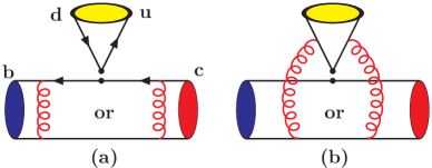
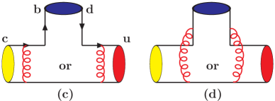
Figure 1: The topologies (a)[(c)] factorizable emission [annihilation] and (b)[(d)] nonfactorizable effects for the decays $B_{d}\to D^{*-}_{0}\pi^{+}$.

There are two topologies in this decay, emission and annihilation diagrams. The former is color-allowed but the latter belongs to color-suppressed. The corresponding flavor diagrams are illustrated by Fig. 1. Hence, the decay amplitude of $B_{d}\to D^{*-}_{0}\pi^{+}$ can be expressed by

$${\cal A}(B_{d}\to D^{*-}_{0}\pi^{+})=f_{\pi}F_{BD^{*}_{0}}+M_{BD^{*}_{0}}+f_{B}F_{a}+M_{a},$$ (10)

where $f_{\pi}$ and $f_{B}$ are the decay constants of $\pi$ and $B$ mesons and the related contributions are the factorizable emission and annihilation topologies, respectively. The remains denote nonfactorizable contributions. With factorization theorem and hadronic structures of Eqs. (3) and (6), the hard amplitudes $\{F\}$ and $\{M\}$ are formulated as

$$F_{BD^{*}_{0}} = 8\pi C_{F}m^{2}_{B}\int_{0}^{1}dx_{1}dx_{2}\int_{0}^{\infty}b_{1}db_{1}b_{2}db_{2}\Phi_{B}(x_{1},b_{1})$$ (11)

$$\times\Big{\{}\Phi_{D1}(x_{2},b_{2}){\cal E}_{D^{*}_{0}}^{1}(t^{(1)}_{e})h_{e}(x_{1},x_{2},b_{1},b_{2})$$

$$+(r_{c}\Phi_{D1}(x_{2})+2r_{2}\Phi_{D2}(x_{2})){\cal E}_{D^{*}_{0}}^{2}(t^{(2)}_{e})h_{e}(x_{2},x_{1},b_{2},b_{1})\Big{\}}$$

$$M_{BD^{*}_{0}} = 16\pi C_{F}m_{B}^{2}\sqrt{2N_{c}}\int_{0}^{1}dx_{1}dx_{2}dx_{3}\int_{0}^{\infty}b_{1}db_{1}b_{3}db_{3}\Phi_{B}(x_{1},b_{1})$$ (12)

$$\times\Phi_{\pi}(x_{3})\Phi_{D1}(x_{2},b_{1})\Big{\{}-(x_{2}+x_{3}){\cal E}_{D^{*}_{0}}^{\prime 1}(t^{(1)}_{d})h^{(1)}_{d}(\{x\},b_{1},b_{3})$$

$$+(1-x_{3}){\cal E}_{D^{*}_{0}}^{\prime 2}(t^{(2)}_{d})h^{(2)}_{d}(\{x\},b_{1},b_{3})\Big{\}},$$

$$F_{a} = 8\pi C_{F}m^{2}_{B}\int_{0}^{1}dx_{2}dx_{3}\int_{0}^{\infty}b_{2}db_{2}db_{3}\Phi_{D1}(x_{2},b_{2})\Phi_{\pi}(\zeta)$$ (13)

$$\Big{\{}-x_{3}{\cal E}_{a}^{1}(t^{(1)}_{a})h_{a}(x_{2},x_{3}\eta_{3},b_{2},b_{3})+x_{2}{\cal E}_{a}^{2}(t^{(2)}_{a})h_{a}(x_{3},x_{2}\eta_{3},b_{3},b_{2})\Big{\}},$$

$$M_{a} = 16\pi C_{F}m_{B}^{2}\sqrt{2N_{c}}\int_{0}^{1}d[x]\int_{0}^{\infty}[b]d[b]\Phi_{B}(x_{1},b_{1})\Phi_{D1}(x_{2},b_{2})\Phi_{\pi}(\zeta)$$ (14)

$$\times\Big{\{}x_{3}{\cal E}_{a}^{\prime 1}(t^{(1)}_{f})h^{(1)}_{f}(\{x\},b_{1},b_{2})-x_{2}{\cal E}_{a}^{\prime 2}(t^{(2)}_{f})h^{(2)}_{f}(\{x\},b_{1},b_{2})\Big{\}}.$$

The hard functions $h_{e(d,a,f)}$, related to the propagators of exchange hard gluon and internal quark, are described by

$$h_{e}(x_{1},x_{2},b_{1},b_{2}) = S_{t}(x_{2})K_{0}\left(\sqrt{x_{1}x_{2}}m_{B}b_{1}\right)$$

$$\times\left[\theta(b_{1}-b_{2})K_{0}\left(\sqrt{x_{2}}m_{B}b_{1}\right)I_{0}\left(\sqrt{x_{2}}m_{B}b_{2}\right)\right.$$

$$\left.+\theta(b_{2}-b_{1})K_{0}\left(\sqrt{x_{2}}m_{B}b_{2}\right)I_{0}\left(\sqrt{x_{2}}m_{B}b_{1}\right)\right]\;,$$

$$h^{(j)}_{d}(x_{1},x_{2},x_{3},b_{1},b_{2}) = \left[\theta(b_{1}-b_{2})K_{0}\left(\sqrt{x_{1}x_{2}}m_{B}b_{1}\right)I_{0}\left(\sqrt{x_{1}x_{2}}m_{B}b_{2}\right)\right.$$

$$\quad\left.+\theta(b_{2}-b_{1})K_{0}\left(\sqrt{x_{1}x_{2}}m_{B}b_{2}\right)I_{0}\left(\sqrt{x_{1}x_{2}}m_{B}b_{1}\right)\right]$$

$$\times\left(\begin{array}[]{cc}K_{0}(D_{j}m_{B}b_{2})&\mbox{for $D^{2}_{j}\geq 0$}\\ \frac{i\pi}{2}H_{0}^{(1)}(\sqrt{|D_{j}^{2}|}m_{B}b_{2})&\mbox{for $D^{2}_{j}\leq 0$}\end{array}\right),$$

$$h_{a}(x_{2},x_{3},b_{2},b_{3}) = S_{t}(x_{3})\left(i\frac{\pi}{2}\right)^{2}H_{0}^{(1)}\left(\sqrt{x_{2}x_{3}}m_{B}b_{2}\right)$$

$$\times\left[\theta(b_{2}-b_{3})H_{0}^{(1)}\left(\sqrt{x_{3}}m_{B}b_{2}\right)J_{0}\left(\sqrt{x_{3}}m_{B}b_{3}\right)\right.$$

$$\left.+\theta(b_{3}-b_{2})H_{0}^{(1)}\left(\sqrt{x_{3}}m_{B}b_{3}\right)J_{0}\left(\sqrt{x_{3}}m_{B}b_{2}\right)\right],$$

$$h^{(j)}_{f}(\{x\},b_{1},b_{2}) = i\frac{\pi}{2}\left[\theta(b_{1}-b_{2})H_{0}^{(1)}\left(\sqrt{x_{2}x_{3}\eta_{3}}m_{B}b_{1}\right)J_{0}\left(\sqrt{x_{2}x_{3}\eta_{3}}m_{B}b_{2}\right)\right.$$

$$\quad\left.+\theta(b_{2}-b_{1})H_{0}^{(1)}\left(\sqrt{x_{2}x_{3}\eta_{3}}m_{B}b_{2}\right)J_{0}\left(\sqrt{x_{2}x_{3}\eta_{3}}m_{B}b_{1}\right)\right]\;$$

$$\times\left(\begin{array}[]{cc}K_{0}(F_{j}m_{B}b_{1})&\mbox{for $F^{2}_{j}\geq 0$}\\ \frac{i\pi}{2}H_{0}^{(1)}(\sqrt{|F_{j}^{2}|}m_{B}b_{1})&\mbox{for $F^{2}_{j}\leq 0$}\end{array}\right),$$

with $D^{2}_{1}=x_{1}x_{2}-x_{2}x_{3}\eta_{3}$, $D^{2}_{2}=x_{1}x_{2}-x_{2}(1-x_{3})\eta_{3}$, $F^{2}_{1}=(x_{1}-x_{2})x_{3}\eta_{3}$, $F^{2}_{2}=x_{1}+x_{2}+(1-x_{1}-x_{2})x_{3}\eta_{3}$, $\eta_{3}=(1-r^{2}_{2})$ and $r_{c}=m_{c}/m_{B}$. The threshold resummation effect is expressed to be $S_{t}(x)=2^{1+2c}\cdot\Gamma(3/2+c)[x(1-x)]^{c}/(\sqrt{\pi}\Gamma(1+c))$, with $c\approx 0.35$ TLS . The evolution factors ${\cal E}_{D^{*}_{0}}^{i}({\cal E}_{D^{*}_{0}}^{\prime i})$ and ${\cal E}_{a}^{i}({\cal E}_{a}^{\prime i})$ are defined by

$${\cal E}^{i}_{D^{*}_{0}}(t^{(i)}_{e}) = \Big{(}C_{2}(t^{(i)}_{e})+\frac{C_{1}(t^{(i)}_{e})}{N_{c}}\Big{)}\alpha_{s}(t^{(i)}_{e})\exp[-S_{B}-S_{D^{*}_{0}}],$$

$${\cal E}^{\prime i}_{D^{*}_{0}}(t^{(i)}_{d}) = \frac{C_{1}(t^{(i)}_{d})}{N_{c}}\alpha_{s}(t^{(i)}_{d})\exp[-S_{B}-S_{D^{*}_{0}}-S_{\pi}]_{b_{2}=b_{1}},$$

$${\cal E}^{i}_{a}(t^{(i)}_{a}) = \Big{(}C_{1}(t^{(i)}_{a})+\frac{C_{2}(t^{(i)}_{a})}{N_{c}}\Big{)}\alpha_{s}(t^{(i)}_{a})\exp[-S_{D^{*}_{0}}-S_{\pi}]_{b_{3}=b_{2}},$$

$${\cal E}^{\prime i}_{a}(t^{(i)}_{f}) = \frac{C_{2}(t^{(i)}_{f})}{N_{c}}\alpha_{s}(t^{(i)}_{f})\exp[-S_{B}-S_{D^{*}_{0}}-S_{\pi}]_{b_{3}=b_{2}},$$

where the exponents $S_{M}$ ($M=B,D^{*}_{0},\pi$) are the Sudakov factors. From above equations, we see clearly that the emission contributions are color-allowed and dictated by effective coupling of $C_{2}+C_{1}/N_{c}$, while the annihilation contributions are color-suppressed and governed by $C_{1}+C_{2}/N_{c}$. $t^{(i)}_{e,d,a,f}$ denote the hard scales of the involving diagrams which are expected to be of ${\cal O}(\sqrt{\bar{\Lambda}m^{2}_{B}})\sim 1.6$ GeV in average and the criteria to determine them are adopted to be

$$t_{e}^{(1)} = {\rm max}(\sqrt{x_{2}}m_{B},1/b_{1},1/b_{2}),\;\;\;t_{e}^{(2)}={\rm max}(\sqrt{x_{1}}m_{B},1/b_{1},1/b_{2}),$$

$$t_{d}^{(j)} = {\rm max}(\sqrt{x_{1}x_{2}}m_{B},\sqrt{D^{2}_{j}}m_{B},1/b_{1},1/b_{3}),$$

$$t_{a}^{(1)} = {\rm max}(\sqrt{x_{3}}m_{B},1/b_{2},1/b_{3}),\;\;\;t_{a}^{(2)}={\rm max}(\sqrt{x_{2}}m_{B},1/b_{2},1/b_{3}),$$

$$t_{f}^{(j)} = {\rm max}(\sqrt{x_{2}x_{3}\eta_{3}}m_{B},\sqrt{F_{j}^{2}}m_{B},1/b_{1},1/b_{2}).$$ (17)

Since we deal with the hadronic effects of the $B$ decay by considering six-quark simultaneously, at lowest order in strong interaction, besides the renormalization group (RG) running from $m_{W}$ to $m_{B}$ scales in the $\mu$-scale dependence of WCs, we still need to consider the running from $m_{B}$ scale to the hard scale $t^{(i)}_{e,d,a,f}$ which indeed dictate the scale of the $B$ meson decay. Hence, in our consideration, the hard scales for WCs are determined by Eq. (17) rather than at $m_{B}$ or $m_{B}/2$ scale. In the formulations of Eqs. (11)$-$(14), we have dropped the terms related to $r^{2}_{2}$ ($r_{c}$ and $r^{2}_{2}$) for the right-handed (left-handed) gluon exchange of Fig. 1. Compared to leading power, which isn’t suppressed by $1/m_{B}$, they all belong to higher power effects.

${\it 2.\ B_{d}\to\bar{D}^{*0}_{0}\pi^{0}\ decay:}$

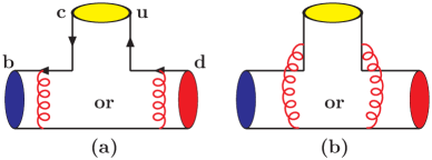
Figure 2: The topologies (a) factorizable emission and (b) nonfactorizable effects for the decays $B_{d}\to\bar{D}^{*0}_{0}\pi^{0}$.

In this decay, the involving annihilation contributions are the same as the decay $B_{d}\to D^{*-}_{0}\pi^{+}$ but the emission topologies become color-suppressed, illustrated by Fig. 2. Due to the neutral pion meson being described by $(\bar{u}u-\bar{d}d)/\sqrt{2}$, the sign of emission topologies is opposite to that of annihilation topologies. Therefore, the decay amplitude is written as

$${\cal A}(B_{d}\to\bar{D}^{*0}_{0}\pi^{0})=\frac{1}{\sqrt{2}}\Big{[}-f_{D^{*}_{0}}F_{B\pi}-M_{B\pi}+f_{B}F_{a}+M_{a}\Big{]},$$ (18)

With the same approach and power counting for the $B_{d}\to D^{*-}_{0}\pi^{+}$ decay, the relevant hard amplitudes $F_{B\pi}(M_{B\pi})$ can be derived as

$$F_{B\pi} = 8\pi C_{F}m^{2}_{B}\int_{0}^{1}dx_{1}dx_{3}\int_{0}^{\infty}b_{1}db_{1}b_{3}db_{3}\Phi_{B}(x_{1},b_{1})$$ (19)

$$\times\Big{\{}\Big{[}(1+x_{3})\Phi_{\pi}(x_{3})+r_{\pi}(1-2x_{3})(\Phi^{p}_{\pi}(x_{3})+\Phi^{\sigma}_{\pi}(x_{3}))\Big{]}{\cal E}_{\pi}^{3}(t^{(3)}_{e})$$

$$\times h_{e}(x_{1},x_{3}\eta_{3},b_{1},b_{3})+2r_{\pi}\Phi^{p}_{\pi}(x_{3}){\cal E}_{\pi}^{4}(t^{(4)}_{e})h_{e}(x_{3},x_{1}\eta_{3},b_{3},b_{1})\Big{\}},$$

$$M_{B\pi} = 16\pi C_{F}m_{B}^{2}\sqrt{2N_{c}}\int_{0}^{1}dx_{1}dx_{2}dx_{3}\int_{0}^{\infty}b_{1}db_{1}b_{2}db_{2}\Phi_{B}(x_{1},b_{1})\Phi_{D1}(x_{2},b_{2})$$ (20)

$$\times\Big{\{}\Big{[}-(x_{2}+x_{3})\Phi_{\pi}(x_{3})+r_{\pi}x_{3}(\Phi^{p}_{\pi}(x_{3})+\Phi^{\sigma}_{\pi}(x_{3}))\Big{]}$$

$$\times{\cal E}_{\pi}^{\prime 3}(t^{(3)}_{d})h^{(3)}_{d}(x_{1},x_{3}\eta_{3},x_{2},b_{1},b_{2})$$

$$+\Big{[}(1-x_{2})\Phi_{\pi}(x_{3})-r_{\pi}x_{3}(\Phi^{p}_{\pi}(x_{3})+\Phi^{\sigma}_{\pi}(x_{3}))\Big{]}$$

$$\times{\cal E}_{\pi}^{\prime 4}(t^{(4)}_{d})h^{(4)}_{d}(x_{1},x_{3}\eta_{3},x_{2},b_{1},b_{2})\Big{\}}.$$

The evolution factors ${\cal E}_{\pi}^{i}({\cal E}_{\pi}^{\prime i})$ are defined by

$${\cal E}^{i}_{\pi}(t^{(i)}_{e}) = \Big{(}C_{1}(t^{(i)}_{e})+\frac{C_{2}(t^{(i)}_{e})}{N_{c}}\Big{)}\alpha_{s}(t^{(i)}_{e})\exp[-S_{B}-S_{\pi}],$$

$${\cal E}^{\prime i}_{\pi}(t^{(i)}_{d}) = \frac{C_{2}(t^{(i)}_{d})}{N_{c}}\alpha_{s}(t^{(i)}_{d})\exp[-S_{B}-S_{D^{*}_{0}}-S_{\pi}]_{b_{3}=b_{1}}.$$

From above equations, due to the appearance of $C_{1}+C_{2}/N_{c}$, we know that $B_{d}\to\bar{D}^{*0}_{0}\pi^{0}$ is color-suppressed process. We note that although nonfactorizable effects are also color-suppressed, since $C_{2}/N_{c}$ could be larger than $C_{1}+C_{2}/N_{c}$, the nonfactorizable effects play a important role in this kind of color-suppressed processes. In fact, the same thing also happens in the decay $B_{d}\to\bar{D}^{0}\pi^{0}$ with $\bar{D}^{0}$ being charmed pseudoscalar PQCD-Group . The hard scales are determined by

$$t_{e}^{(3)} = {\rm max}(\sqrt{x_{3}\eta_{3}}m_{B},1/b_{1},1/b_{3})\;,\;\;\;t_{e}^{(4)}={\rm max}(\sqrt{x_{1}\eta_{3}}m_{B},1/b_{1},1/b_{3})\;,$$

$$t_{d}^{(3)} = {\rm max}(\sqrt{x_{1}x_{3}\eta_{3}}m_{B},\sqrt{D^{2}_{3}}m_{B},1/b_{1},1/b_{2}),$$

$$t_{d}^{(4)} = {\rm max}(\sqrt{x_{1}x_{3}\eta_{3}}m_{B},\sqrt{D^{2}_{4}}m_{B},1/b_{1},1/b_{2}),$$

with $D^{2}_{3}=(x_{1}-x_{2})x_{3}\eta_{3}$ and $D^{2}_{4}=(x_{1}+x_{2})r^{2}_{2}-(1-x_{1}-x_{2})x_{3}\eta_{3}$.

${\it 3.\ B^{+}\to\bar{D}^{*0}_{0}\pi^{+}\ decay:}$

In this decay, there are no annihilation contributions and new topologies involved. The corresponding flavor diagrams are the same as Fig. 1(a) and (b) and Fig. 2. Hence, we can immediately write the decay amplitude as

$${\cal A}(B^{+}\to\bar{D}^{*0}_{0}\pi^{+})=f_{\pi}F_{BD^{*}_{0}}+M_{BD^{*}_{0}}+f_{D^{*}_{0}}F_{B\pi}+M_{B\pi}.$$ (21)

The hard amplitudes $\{F\}$ and $\{M\}$ are the same as Eqs. (11), (12), (19) and (20).

IV Numerical analysis

In our calculations, we adopt the $B$-meson wave function $\Phi_{B}$ to be

$$\Phi_{B}(x,b) = N_{B}x^{2}(1-x)^{2}\exp\Big{[}-\frac{1}{2}\Big{(}\frac{x\,m_{B}}{\omega_{B}}\Big{)}^{2}-\frac{\omega_{B}^{2}b^{2}}{2}\Big{]},$$ (22)

where $N_{B}$ can be determined by the normalization of the wave function at $b=0$ and $\omega_{B}$ is the shape parameter. Since the $\pi$-meson wave functions have been derived in the framework of QCD sum rules, we display them up to twist-3 directly by Ball

$$\Phi_{\pi}(x) = \frac{3f_{\pi}}{\sqrt{2N_{c}}}x(1-x)\left[1+0.44C_{2}^{3/2}(2x-1)+0.25C_{4}^{3/2}(2x-1)\right],$$

$$\Phi_{\pi}^{p}(x) = \frac{f_{\pi}}{2\sqrt{2N_{c}}}\left[1+0.43C_{2}^{1/2}(2x-1)+0.09C_{4}^{1/2}(2x-1)\right],$$

$$\Phi_{\pi}^{\sigma}(x) = \frac{f_{\pi}}{2\sqrt{2N_{c}}}(1-2x)\left[1+0.55(10x^{2}-10x+1)\right],$$

with the Gegenbauer polynomials,

$$C_{2}^{1/2}(\xi) = \frac{1}{2}(3\xi^{2}-1),\;\;\;\;\;C_{4}^{1/2}(\xi)=\frac{1}{8}(35\xi^{4}-30\xi^{2}+3),$$

$$C_{2}^{3/2}(\xi) = \frac{3}{2}(5\xi^{2}-1),\;\;\;\;\;C_{4}^{3/2}(\xi)=\frac{15}{8}(21\xi^{4}-14\xi^{2}+1).$$

After the wave functions of $\pi$ meson are determined, the unknown $\omega_{B}$ can be fixed by decays such as $B\to\pi\pi$. Consequently, the remaining uncertain parameters are the wave functions of the $D^{*}_{0}$ meson.

To obtain the numerical results, the values of theoretical inputs are chosen as: $\omega_{B}=0.4$, $f_{B}=0.19$, $f_{\pi}=0.13$, $\tilde{f}_{D^{*}_{0}}=0.20$, $m_{B}=5.28$, $m_{D^{*}_{0}}=2.29$, and $m^{0}_{\pi}=1.4$ GeV. With these values, we get the form factor $F^{B\to\pi}(0)=0.3$. In addition, the values of $B\to D^{*}_{0}$ form factor with some variances in $a_{D^{*}_{0}}$ and $\omega_{D^{*}_{0}}$ are also shown in Table 1.

Table 1: The values of $B\to D^{*}_{0}$ form factor with $b_{D^{*}_{0}}=0.5$ and some variances in $a_{D^{*}_{0}}$ and $\omega_{D^{*}_{0}}$.

$\omega_{D^{*}_{0}}$	$a_{D^{*}_{0}}=0.7$	$a_{D^{*}_{0}}=0.9$	$a_{D^{*}_{0}}=1.1$
$0.5$	$0.29$	$0.30$	$0.31$
$0.6$	$0.24$	$0.25$	$0.26$
$0.7$	$0.21$	$0.22$	$0.23$

It is interesting that the form factor of $B\to D^{*}_{0}$ decay is much smaller than that of $B\to D$ decay, which is calculated to be around $0.57$ PQCD-Group . We also find that our results are a little bit larger than those calculated by ISGW2 model Cheng2 . According to Wolfenstein’s parametrization Wolfenstein , we take $A=0.82$ and $\lambda=0.22$ for the CKM matrix element $V_{cb}=A\lambda^{2}$. Hence, in terms of our deriving formulas and by fixing $a_{D^{*}_{0}}=0.9$, $b_{D^{*}_{0}}=0.5$ and $\omega_{D^{*}_{0}}=0.6$, the magnitudes of the hard amplitudes are shown in Table 2.

Table 2: The values of hard amplitudes (in units of $10^{-3}$) with fixing $a_{D^{*}_{0}}=0.9$, $b_{D^{*}_{0}}=0.5$ and $\omega_{D^{*}_{0}}=0.6$.

$f_{\pi}F_{BD^{*}_{0}}$	$M_{BD^{*}_{0}}$	$f_{B}F_{a}$	$M_{a}$	$f_{D^{*}_{0}}F_{B\pi}$	$M_{B\pi}$
$36.4$	$10^{-2}(1.0-i3.2)$	$-0.06-i0.08$	$-1.85-i3.14$	$-7.11$	$7.56-i10.95$

From the table, we can see clearly that except $M_{BD^{*}_{0}}$, the nonfactorizable effects of color-suppressed process are comparable to factorizable contributions; even in annihilation topologies, the contributions of the former are much larger than those of the latter. With fixing $b_{D^{*}_{0}}=0.5$ and $\omega_{D^{*}_{0}}=0.6$ GeV and taking some different values of $a_{D^{*}_{0}}$, the decay BRs of $B\to D^{*}_{0}\pi$ are displayed in Table 3. We also show the BRs with fixing $a_{D^{*}_{0}}=0.9$ and $b_{D^{*}_{0}}=0.5$ and some variant values of $\omega_{D^{*}_{0}}$. From both tables, we know that with proper values of parameters, the calculated BR of $B^{+}\to D^{*0}_{0}\pi^{+}$ is consistent with the BELLE’s observation. It is worth to note that the predicted BR of $B_{d}\to\bar{D}^{*0}_{0}\pi^{0}$ is one order of magnitude smaller than others. The phenomenon can be understood by noticing that, as shown in Table 2, the value of $F_{B\pi}$ is very close and opposite in sign to the real part of $M_{B\pi}$ such that there is a strong cancellation in Eq. (18). As a result, we get the small BR in the decay $B_{d}\to\bar{D}^{*0}_{0}\pi^{0}$. That is, the annihilation effects are significant in $B\to\bar{D}^{*0}_{0}\pi^{0}$.

Table 3: The BRs (in units of $10^{-4}$) with fixing $b_{D^{*}_{0}}=0.5$, $\omega_{D^{*}_{0}}=0.6$ GeV and various values of $a_{D^{*}_{0}}$.

$a_{D_{s}}$	$B^{+}\to\bar{D}^{*0}_{0}\pi^{+}$	$B_{d}\to D^{*-}_{0}\pi^{+}$	$B_{d}\to\bar{D}^{*0}_{0}\pi^{0}$
1.1	9.75	8.25	0.17
0.9	9.34	7.68	0.19
0.7	8.98	7.13	0.21

Table 4: The BRs (in units of $10^{-4}$) with fixing $a_{D^{*}_{0}}=0.9$ and $b_{D^{*}_{0}}=0.5$ and various values of $\omega_{D^{*}_{0}}$.

$\omega_{D^{*}_{0}}$	$B^{+}\to\bar{D}^{*0}_{0}\pi^{+}$	$B_{d}\to D^{*-}_{0}\pi^{+}$	$B_{d}\to\bar{D}^{*0}_{0}\pi^{0}$
0.5	13.79	10.7	0.26
0.6	9.34	7.68	0.19
0.7	6.28	5.55	0.15

As stated before, although we only study the decays $B\to D^{*}_{0}\pi$, we still can estimate the BRs of $B\to D^{(\prime)}_{1}\pi$. Since only the longitudinal polarization has the contributions, except the decay constants, we expect that the involving wave functions of $D^{(\prime)}_{1}$ should be similar to $D^{*}_{0}$. By neglecting the difference in phase space, the BRs of $B\to D^{(\prime)}_{1}\pi$ could be estimated by $BR(B\to D^{(\prime)}_{1}\pi)/BR(B\to D^{*}_{0}\pi)\sim(\tilde{f}_{D^{(\prime)}_{1}}/\tilde{f}_{D^{*}_{0}})^{2}$. If $\tilde{f}_{D^{(\prime)}_{1}}\approx\tilde{f}_{D^{*}_{0}}$, the BRs for producing axial vector mesons $D^{(\prime)}_{1}$ are close to that for the scalar $D^{*}_{0}$. The tendency is consistent with BELLE’s observations, shown in Eq. (2).

V Summary

We have studied the properties of $P$-wave mesons in $B$ decays in terms of $D^{*}_{0}$. By taking the concept of the heavy quark limit, we have obtained some information on the shapes of $D^{*}_{0}$ wave functions. According to the wave function of $K^{*}_{0}(1420)$, we can determine the proper value for the parameter $a_{D^{*}_{0}}$ in $\Phi_{D1}(x)$. By the physical argument, the unknown parameter $b_{D^{*}_{0}}$ can be chosen so that the maximum of $\Phi_{D2}(x)$ locates at $x\sim 0.35$. We have found that with a suitable value of $\omega_{D^{*}_{0}}$, our result on $BR(B^{+}\to\bar{D}^{*0}_{0}\pi^{+})$ can fit BELLE’s measurements. Hence, the calculated BRs for $B_{d}\to D^{*-}_{0}\pi^{+}$ and $B_{d}\to\bar{D}^{*0}_{0}\pi^{0}$ decays can be viewed as our predictions. Finally, if we regard that the longitudinal wave functions of $D^{(\prime)}_{1}$ are the same as $D^{(*)}_{0}$ and assume that $\tilde{f}_{D^{(\prime)}_{1}}\approx\tilde{f}_{D^{*}_{0}}$, we expect that the differences of BRs among them are not significant. The more accurate predictions rely on more definite values of decay constants as well as other unknown parameters.

Acknowledgments

The authors would like to thank C.Q. Geng, H.N. Li, H.Y. Cheng and Taekoon Lee for their useful discussions. This work is supported in part by the National Science Council of the Republic of China under Grant No. NSC-91-2112-M-001-053 and the National Center for Theoretical Sciences of R.O.C..

References

• (1) H.Y. Cheng, Phys. Rev. D67, (2003) 034024.
• (2) R.J. Jaffe, Phys. Rev. D15, (1977) 267; ibid, 281 (1997); M. Alford and R.J. Jaffe, Nucl. Phys. B578, (2000) 367.
• (3) BABAR Collaboration, B. Aubert et al., Phys. Rev. Lett. 90, 242001 (2003).
• (4) CLEO Collaboration, D. Besson et al., hep-ex/0305017.
• (5) BELLE Collaboration, presented by T.Browder at 8th Conference on the Intersections of Particle and Nuclear Physics, held on 19 - 24, May 2003, New York, New York, USA.
• (6) S. Godfrey and N. Isgur, Phys. Rev. D32, (1985) 189 ; S. Godfrey and R. Kokoski, Phys. Rev. D43, (1991) 1679; D. Ebert, V.O. Galkin and R.N. Faustov, Phys. Rev. D57, (1998) 5663; Erratum-ibid. D59, (1999) 019902; M. Di Pierro and E. Eichten, Phys. Rev. D64, (2001) 114004; T. A. Lahde, C. J. Nyfalt and D. O. Riska, Nucl. Phys. A674, (2000) 141; R. Lewis and R.M. Woloshyn, Phys. Rev. D62, (2000) 114507; G. S. Bali, hep-ph/0305209.
• (7) W.A. Bardeen, E.J. Eichten and C.T. Hill, hep-ph/0305049.
• (8) R.N. Cahn and J.D. Jackson, Phys. Rev. D68, 037502 (2003).
• (9) T. Barnes, F.E. Close and H.J. Lipkin, Phys. Rev. D68, 054006 (2003).
• (10) E. van Beveren and G. Rupp, Phys. Rev. Lett. 91, 012003 (2003).
• (11) Hai-Yang Cheng and Wei-Shu Hou, Phys. Lett. B566, 193 (2003).
• (12) A.P. Szczepaniak, Phys. Lett. B567, 23 (2003).
• (13) P. Colangelo and F. De Fazio, Phys. Lett. B570, 180 (2003).
• (14) C.H. Chen and H.N. Li, hep-ph/0307075.
• (15) CLEO Collaboration, J. Gronberg et al., CLEO CONF 96-25, ICHEP96 PA05-069.
• (16) BELLE Collaboration, K. Abe et al., BELLE-CONF-0235, ICHEP02 Parallel 8.
• (17) BELLE Collaboration, presented by T. Karim at Flavor Physics $\&$ CP Violation FPCP 2003, held on 3-6 June 2003 - Ecole Polytechnique, Paris, France; hep-ex/0307021.
• (18) G.P. Lepage and S.J. Brodsky, Phys. Lett. B87, (1979) 359; Phys. Rev. D22, (1980) 2157.
• (19) H.N. Li, Phys. Rev. D64, (2001) 014019.
• (20) J.D. Bjorken, Topics in $B$-physics, Nucl. Phys. 11 (Proc. Suppl.), (1989) 325.
• (21) T. Kurimoto, H.N. Li and A.I. Sanda, Phys. Rev. D67, 054028 (2003).
• (22) Y.Y. Keum, T. Kurimoto, H.N. Li, C.-D. Lu and A.I. Sanda, hep-ph/0305335.
• (23) Particle Data Group, K. Hagiwara et al., Phys. Rev. D66, (2002) 010001.
• (24) T. Kurimoto, H.N. Li and A.I. Sanda, Phys. Rev. D65, (2002) 014007; C.H. Chen, Y.Y. Keum and H.N. Li, Phys. Rev. D66, (2002) 054013.
• (25) P. Ball, J. High Energy Phys. 01, (1999) 010.
• (26) K. Maltman, Phys. Lett. B462, (1999) 14.
• (27) S. Veseli and I. Dunietz, Phys. Rev. D11, (1996) 6803.
• (28) M. Diehl and G. Hiller, JHEP06, (2001) 067.
• (29) H. Y. Cheng, hep-ph/0307168.
• (30) N. Cabibbo, Phys. Rev. Lett. 10, (1963) 531; M. Kobayashi and T. Maskawa, Prog. Theor. Phys. 49, (1973) 652.
• (31) G. Buchalla , A.J. Buras and M.E. Lautenbacher, Rev. Mod. Phys. 68, (1996) 1230.
• (32) T. Kurimoto, H-n. Li, and A.I. Sanda, Phys. Rev. D 65, (2002) 014007.
• (33) L. Wolfenstein, Phys. Rev. Lett. 51, (1983) 1841.