$J/\psi$ couplings to open charm mesons from QCD sum rules

Abstract

We employ QCD sum rules to calculate the $J/\psi$ form factors and coupling constants with charmed mesons, by studying three-point correlation functions. In particular we consider the $J/\psi D^{*}D$ and $J/\psi DD$ vertices. We determine the momentum dependence of the form factors for kinematical conditions where $J/\psi,~{}D$ or $D^{*}$ are off-shell. Extrapolating to the pole of each one of the so obtained form factors, we determine the coupling constants. For both couplings our results (within the errors) are compatible with estimates based on constituent quark model.

I Introduction

Since their begining in 1998, effective Lagrangian theories for charmed mesons were constructed to give us a better understanding of the interaction between $J/\psi$ and light mesons in nuclear matter. Although the original motivation is still very strong, specially in view of the vigorous ongoing RHIC program, this new sub-area of hadron physics introduced new questions which are now in debate. Some of them are: What are the coupling constants involving heavy mesons? Which are the form factors appearing in these vertices? To what extent are we allowed to use SU(4) symmetry? Moreover, interactions of charmed mesons offer a testing ground for the predictions of heavy quark effective theory (HQET) hqet . As pointed out in ref. dea , a consequence of the spin symmetry of HQET is that

$$g_{\psi DD^{*}}={g_{\psi DD}\over m_{D}}.$$ (1)

We will in this work calculate both couplings independently and will have the opportunity to check the relation above.

Charmed hadrons are composites of the underlying quarks whose effective fields describe point-like physics only when all the interacting particles are on mass-shell. When at least one of the particles in a vertex is off-shell, the finite size effects of hadrons become important. Therefore, the knowledge of form factors in hadronic vertices is of crucial importance to estimate any amplitude using hadronic degrees of freedom. This work is devoted to the study of the $J/\psi D^{*}D$ form factor, which is important, for instance, in the evaluation of the dissociation cross section of $J/\psi$ by pions and $\rho$ mesons using effective Lagrangians osl ; nnr ; haga2 .

The $J/\psi D^{*}D$ coupling has been studied by some authors using different approaches: vector meson dominance model plus relativistic potential model osl and constituent quark models dea . Unfortunately, the numerical results from these calculations may differ by almost a factor two. The relevance of this difference can not be underestimated since the cross sections are proportional to the square of the coupling constants. In ref. haga2 it was shown that the use of different coupling constants and form factors can lead to cross sections that differ by more than one order of magnitude, and that can even have a different behavior as a function of $\sqrt{s}$.

In previous works we have used the QCD sum rules (QCDSR) to study the $D^{*}D\pi$ nos1 ; nos2 , $DD\rho$ nos4 and $J/\psi DD$ nos3 form factors, considering two different mesons off mass-shell. In these works the QCDSR results for the form factors were parametrized by analytical forms such that the respective extrapolations to the off-shell meson poles provided consistent values for the corresponding coupling constant. In this work we use the QCDSR approach to evaluate the $J/\psi D^{*}D$ form factors and extend the procedure described above to estimate the $J/\psi D^{*}D$ coupling constant considering each one of these mesons off-shell, calculating the associated form factor, and then extrapolating the three obtained form factors to the corresponding on-shell masses. We will apply this method to both $J/\psi DD$ and $J/\psi D^{*}D$ vertices.

II The QCD sum rule approach

The three-point function associated with the hadronic vertex $J/\psi DD^{*}$, where $J/\psi$ and $D$ are the incoming and outgoing external mesons with momentum $p$ and $p^{\prime}$ respectively and $D^{*}$ is the off-shell meson, with momentum $q=p^{\prime}-p$ is given by

$$\Gamma_{\mu\nu}(p,p^{\prime})=\int d^{4}x\,d^{4}y\,\,e^{ip^{\prime}.x}\,e^{-iq.y}\langle 0|T\{j_{D}(x){j_{\nu}^{D^{*}}}^{\dagger}(y){j_{\mu}^{\psi}}^{\dagger}(0)\}|0\rangle\;,$$ (2)

where the interpolating fields are $j_{\mu}^{\psi}=\bar{c}\gamma_{\mu}c$, $j_{\nu}^{D^{*}}=\bar{q}\gamma_{\nu}c$ and $j_{D}=i\bar{q}\gamma_{5}c$ with $q$ and $c$ being a light quark and the charm quark fields.

The fundamental assumption of the QCD sum rule approach svz ; rry is the principle of duality, i.e., it is assumed that there is an interval over which a correlation function may be equivalently described at the quark level and at the hadron level. Therefore, the procedure of the QCD sum rule technique is the following: on one hand we calculate the correlator in Eq.(2) at the quark level in terms of quark and gluon fields. On the other hand, the correlator is calculated at the hadronic level introducing hadron characteristics, giving sum rules from which a hadronic quantity can be estimated.

The hadronic side of the correlation function, $\Gamma_{\mu\nu}(p,p^{\prime})$, is obtained by the consideration of $J/\psi$, $D^{*}$ and $D$ state contributions to the matrix element in Eq. (2):

$$\Gamma_{\mu\nu}^{(phen)}(p,p^{\prime})={m_{D}^{2}f_{D}\over m_{c}}m_{D^{*}}f_{D^{*}}m_{\psi}f_{\psi}{g_{\psi DD*}^{(D^{*})}(q^{2})\epsilon_{\alpha\beta\mu\nu}p^{\alpha}{p^{\prime}}^{\beta}\over(q^{2}-m_{D^{*}}^{2})(p^{2}-m_{\psi}^{2})({p^{\prime}}^{2}-m_{D}^{2})}+\mbox{h.~{}r.}\;,$$ (3)

where h. r. means higher resonances.

The meson decay constants appearing in Eq. (3) are defined by the vacuum to meson transition amplitudes:

$$\langle 0|j^{(D)}|D\rangle={m_{D}^{2}f_{D}\over m_{c}}\;,$$ (4)

and

$$\langle V(p,\epsilon)|j^{\dagger}_{\alpha}|0\rangle=m_{V}f_{V}\epsilon^{*}_{\alpha}\;,$$ (5)

for the vector mesons $V=J/\psi$ and $V=D^{*}$. The form factor we want to estimate is defined through the vertex function for an off-shell $D^{*}$ meson:

$$\langle\psi(p,\lambda)|D(p^{\prime})D^{*}(q,\lambda^{\prime})\rangle=g_{\psi DD*}^{(D^{*})}(q^{2})\epsilon^{\alpha\beta\gamma\delta}\epsilon_{\alpha}^{\lambda}(p)\epsilon_{\gamma}^{\lambda^{\prime}}(q)p^{\prime}_{\beta}q_{\delta}\;.$$ (6)

The contribution of higher resonances and continuum in Eq. (3) will be taken into account as usual in the standard form of ref. io2 .

The QCD side, or theoretical side, of the correlation function is evaluated by performing Wilson’s operator product expansion (OPE) of the operator in Eq. (2). Writing $\Gamma_{\mu\nu}$ in terms of the invariant amplitude:

$$\Gamma_{\mu\nu}(p,p^{\prime})=\Lambda(p^{2},{p^{\prime}}^{2},q^{2})\epsilon_{\alpha\beta\mu\nu}p^{\alpha}{p^{\prime}}^{\beta}\;,$$ (7)

we can write a double dispersion relation for $\Lambda$, over the virtualities $p^{2}$ and ${p^{\prime}}^{2}$ holding $q^{2}$ fixed:

$$\Lambda(p^{2},{p^{\prime}}^{2},q^{2})=-{1\over 4\pi^{2}}\int dsdu~{}{\rho(s,u,q^{2})\over(s-p^{2})(u-{p^{\prime}}^{2})}\;,$$ (8)

where $\rho(s,u,q^{2})$ equals the double discontinuity of the amplitude $\Lambda(p^{2},{p^{\prime}}^{2},q^{2})$ on the cuts $4m_{c}^{2}\leq s\leq\infty$, $m_{c}^{2}\leq u\leq\infty$, We consider diagrams up to dimension three which include the perturbative diagram and the quark condensate.

To improve the matching between the two sides of the sum rules, we perform a double Borel transformation in both variables $P^{2}=-p^{2}\rightarrow M^{2}$ and ${P^{\prime}}^{2}=-{p^{\prime}}^{2}\rightarrow{M^{\prime}}^{2}$. We get the following sum rule:

$$C~{}\frac{g_{\psi DD^{*}}^{(D^{*})}(t)}{(t-m_{D^{*}}^{2})}e^{-\frac{m_{D}^{2}}{{M^{\prime}}^{2}}}e^{-\frac{m_{\psi}^{2}}{M^{2}}} = \frac{1}{4\pi^{2}}\int_{4m^{2}}^{s_{0}}\int_{u_{min}}^{u_{0}}dsdu~{}\rho^{(D^{*})}(u,s,t)e^{-\frac{s}{M^{2}}}e^{-\frac{u}{{M^{\prime}}^{2}}}\Theta(u_{max}-u)$$ (9)

$$+ {m_{c}\langle g_{s}^{2}G^{2}\rangle\over 2\pi^{2}}\Pi_{G}(t,M^{2},{M^{\prime}}^{2}),$$

where $C={m_{D}^{2}f_{D}\over m_{c}}m_{D^{*}}f_{D^{*}}m_{\psi}f_{\psi}$, $t=q^{2}$,

$$\rho^{(D^{*})}(u,s,t)=\frac{3m_{c}}{\sqrt{\lambda}}\left(1+\frac{s\lambda_{2}}{\lambda}\right),$$ (10)

with $\lambda=(u+s-t)^{2}-4us$, $\lambda_{2}=u+t-s+2m_{c}^{2}$ and

$$u^{max}_{min}=\frac{1}{2m_{c}^{2}}\left[-st+m_{c}^{2}(s+2t)\pm\sqrt{s(s-4m_{c}^{2})(t-m_{c}^{2})^{2}}\right].$$ (11)

The last term in Eq. (9) gives the gluon condensate contribution. The full expression for the gluon condensate contribution is given in Appendix A.

In Eq. (9) we have transferred to the QCD side the higher resonances contributions through the introduction of the continuum thresholds $s_{0}$ and $u_{0}$. The sum rules for the form factors considering the mesons $J/\psi$ and $D$ as off-shell mesons can be obtained in a similar way. In the case that the $D$ meson is off-shell we get basically the same sum rule, the only difference being the exchange between $m_{D}^{2}$ and $m_{D^{*}}^{2}$ in the left hand side of Eq. (9). The spectral density is exactly the same bjp . In the case that $J/\psi$ is off-shell we get

$$C~{}\frac{g_{\psi DD^{*}}^{(J/\psi)}(t)}{(t-m_{\psi}^{2})}e^{-\frac{m_{D}^{2}}{{M^{\prime}}^{2}}}e^{-\frac{m_{D^{*}}^{2}}{M^{2}}}=\frac{1}{4\pi^{2}}\int_{m^{2}}^{s_{0}}\int_{u_{min}}^{u_{0}}dsdu\rho^{(J/\psi)}(u,s,t)e^{-\frac{s}{M^{2}}}e^{-\frac{u}{{M^{\prime}}^{2}}}\Theta(u_{max}-u),$$ (12)

with

$$\rho^{(J/\psi)}(u,s,t)=\frac{3m_{c}}{\lambda^{3/2}}\left[(u-s)^{2}-t(u+s-2m_{c}^{2})\right]-4\pi^{2}<\bar{q}q>\delta(s-m_{c}^{2})\delta(u-m_{c}^{2}),$$ (13)

and

$$u^{max}_{min}=\frac{1}{2m_{c}^{2}}\left[-st+m_{c}^{2}(2s+t)\pm\sqrt{t(t-4m_{c}^{2})(s-m_{c}^{2})^{2}}\right].$$ (14)

III Form factors in the $J/\psi$ vertices

III.1 $J/\psi DD^{*}$

The parameter values used in all calculations are: $m_{D}=1.87\,\nobreak\,\mbox{GeV}$, $m_{D^{*}}=2.01\,\nobreak\,\mbox{GeV}$, $m_{\psi}=3.1\,\nobreak\,\mbox{GeV}$, $f_{J/\psi}=(405\pm 15)\nobreak\,\mbox{MeV}$ PDG . For $f_{D}$ and $f_{D^{*}}$ we use the values evaluated in the two-point QCD sum rules under the same kind of approximations bbkr : $f_{D}=(170\pm 10)~{}\nobreak\,\mbox{MeV}$, $f_{D^{*}}=(240\pm 20)~{}\nobreak\,\mbox{MeV}$. For the charm quark mass, quark condensate and gluon condensate we use the values normally used in QCD sum rules calculations svz ; rry $m_{c}=1.3\,\nobreak\,\mbox{GeV}$, $\langle\overline{q}q\rangle\,=\,-(0.23)^{3}\,\nobreak\,\mbox{GeV}^{3}$, $\langle g_{s}^{2}G^{2}\rangle\,=\,0.5\,\nobreak\,\mbox{GeV}^{4}$ For the continuum thresholds we take $s_{0}=(m_{\psi}+\Delta_{s})^{2}$ and $u_{0}=(m_{D(D^{*})}+\Delta_{u})^{2}$ for the sum rules when $D(D^{*})$ is off-shell, and $s_{0}=(m_{D^{*}}+\Delta_{s})^{2}$ and $u_{0}=(m_{D}+\Delta_{u})^{2}$ for the sum rule when $J/\psi$ is off-shell. We take $\Delta_{s}=\Delta_{u}=(0.5\pm 0.1)\nobreak\,\mbox{GeV}$.

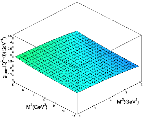
Figure 1: $M^{2}$ and ${M^{\prime}}^{2}$ dependence of $g_{\psi DD^{*}}^{(D^{*})}(Q^{2}=0)$.

We first discuss the $J/\psi DD^{*}$ form factor with an off-shell $D^{*}$ meson. Fixing $Q^{2}=-q^{2}=0$ and $\Delta_{s}=\Delta_{u}=0.5~{}\nobreak\,\mbox{GeV}$ we show in Fig. 1 the Borel dependence of the form factor $g_{\psi DD^{*}}^{(D^{*})}(0)$. We see that we get a very good stability for the form factor as a function of the two independent Borel parameters in the considered Borel regions.

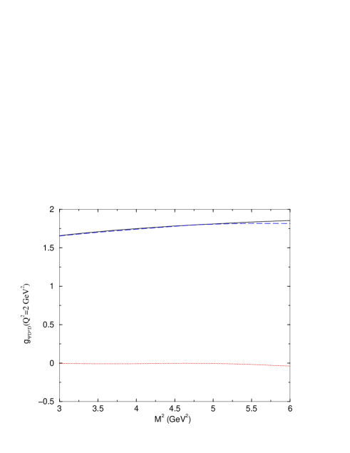
Figure 2: ${M^{\prime}}^{2}$ dependence of perturbative contribution (dashed line) and the gluon condensate contribution (dotted line) to $g_{J/\psi DD^{*}}^{(D^{*})}$ at $Q^{2}=2.0\,\nobreak\,\mbox{GeV}^{2}$. The solid line gives the final reslt for the form factor.

The same kind of stability is obtained for other values of $Q^{2}$ and for the other two form factors bjp .

In Fig. 2 we show the perturbative (dashed line) and the gluon condensate (dotted line) contributions to the form factor $g_{J/\psi DD^{*}}^{(D^{*})}(Q^{2})$ at $Q^{2}=2~{}\nobreak\,\mbox{GeV}^{2}$ as a function of the Borel mass ${M^{\prime}}^{2}$ at a fixed ratio ${M^{\prime}}^{2}/M^{2}={m_{D}^{2}/m_{\psi}^{2}}$. We see that the gluon condensate contribution is negligible, as compared with the perturbative contribution. The same kind of behaviour is obtained for other values of $Q^{2}$. This is a very interesting result since it might be indicating a convergence of the OPE.

In Fig. 3 we show the behavior of the form factors $g_{J/\psi DD^{*}}(Q^{2})$ at $Q^{2}=2~{}\nobreak\,\mbox{GeV}^{2}$ as a function of the Borel mass ${M^{\prime}}^{2}$. The solid line gives $g_{J/\psi DD^{*}}^{(D^{*})}$ at a fixed ratio ${M^{\prime}}^{2}/M^{2}={m_{D}^{2}/m_{\psi}^{2}}$. The dashed line gives $g_{J/\psi DD^{*}}^{(D)}$ at a fixed ratio ${M^{\prime}}^{2}/M^{2}={m_{D^{*}}^{2}/m_{\psi}^{2}}$, and the dotted line gives $g_{J/\psi DD^{*}}^{(J/\psi)}$ at a fixed ratio ${M^{\prime}}^{2}/M^{2}={m_{D}^{2}/m_{D^{*}}^{2}}$.

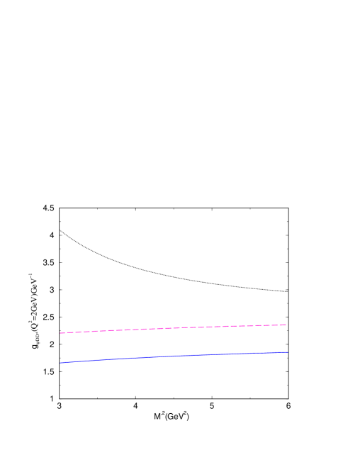
Figure 3: ${M^{\prime}}^{2}$ dependence of $g_{J/\psi DD^{*}}^{(D^{*})}$ (solid line), $g_{J/\psi DD^{*}}^{(D)}$ (dashed line) and $g_{J/\psi DD^{*}}^{(J/\psi)}$ (dotted line) for $Q^{2}=2.0\,\nobreak\,\mbox{GeV}^{2}$.

We can see that the QCDSR results for $g_{J/\psi DD^{*}}^{(D^{*})}$ and $g_{J/\psi DD^{*}}^{(D)}$ are very stable in the interval $3\leq{M^{\prime}}^{2}\leq 6\,\nobreak\,\mbox{GeV}^{2}$. In the case of $g_{J/\psi DD^{*}}^{(J/\psi)}$ the stability is not as good as for the other form factors, but it is still acceptable.

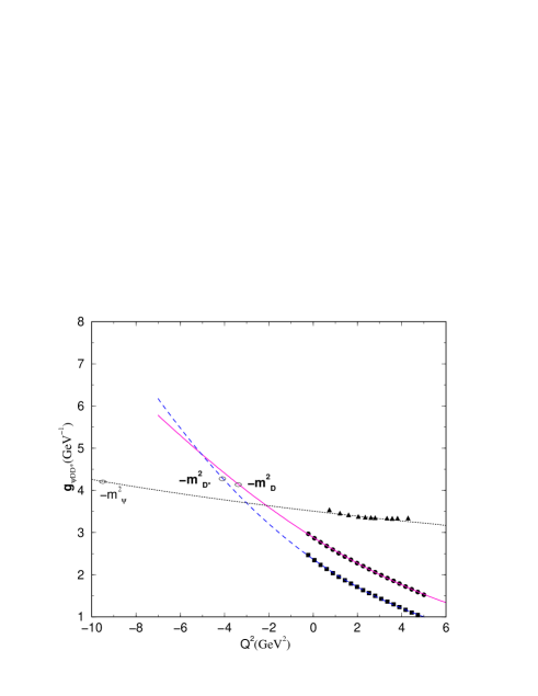
Figure 4: Momentum dependence of the $J/\psi DD^{*}$ form factors. The dotted, dashed and solid lines give the parametrization of the QCDSR results (triangles, squares and circles) through Eqs. (15), (16) and (17) respectively.

Fixing $M^{2}$ and ${M^{\prime}}^{2}$ at the values of the incoming and outgoing meson masses we show, in Fig. 4, the momentum dependence of the QCDSR results for the form factors $g_{\psi DD^{*}}^{(D)}$, $g_{\psi DD^{*}}^{(D^{*})}$ and $g_{\psi DD^{*}}^{(J/\psi)}$ through the circles, squares and triangles respectively. Since the present approach cannot be used at $Q^{2}<<0$, in order to extract the $g_{\psi DD^{*}}$ coupling from the form factors we need to extrapolate the curves to the mass of the off-shell meson, shown as open circles in Fig. 4.

In order to do this extrapolation we fit the QCDSR results with an analytical expression. We tried to fit our results to a monopole form, since this is very often used for form factors, but the fit was only good for $g_{\psi DD^{*}}^{(J/\psi)}$. For $g_{\psi DD^{*}}^{(D)}$ and $g_{\psi DD^{*}}^{(D^{*})}$ we obtained good fits using a Gaussian form. We get:

$$g^{(J/\psi)}_{\psi DD^{*}}(Q^{2})=\frac{200}{57+Q^{2}}=4.2{57-m_{\psi}^{2}\over 57+Q^{2}},$$ (15)

$$g^{(D^{*})}_{\psi DD^{*}}(Q^{2})=20~{}e^{-\frac{(Q^{2}+27)^{2}}{345}},$$ (16)

$$g^{(D)}_{\psi DD^{*}}(Q^{2})=13~{}e^{-\frac{(Q^{2}+26)^{2}}{450}}.$$ (17)

These fits are also shown in Fig. 4 through the dotted, dashed and solid lines respectively. From Fig. 4 we see that all three form factors lead to compatible values for the coupling constant when the form factors are extrapolated to the off-shell meson masses (open circles in Fig. 4).

All results showed above were obtained using $\Delta_{s}=\Delta_{u}=0.5~{}\nobreak\,\mbox{GeV}$. In Fig. 5 we use the form factor $g^{(D)}_{\psi DD^{*}}(Q^{2})$ to ilustrate the dependence of our results with the continuum thresholds.

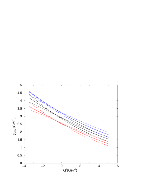
Figure 5: Continuum threshold dependence of the form factor $g^{(D)}_{\psi DD^{*}}(Q^{2})$. The dashed solid and dotted lines give the parametrization of the QCDSR results for $\Delta_{s}=0.4~{}\nobreak\,\mbox{GeV},~{}0.5~{}\nobreak\,\mbox{GeV}$ and $0.6~{}\nobreak\,\mbox{GeV}$ respectively. The lower, intermediate and upper set of curves show the results for $\Delta_{u}=0.4~{}\nobreak\,\mbox{GeV},~{}0.5~{}\nobreak\,\mbox{GeV}$ and $0.6~{}\nobreak\,\mbox{GeV}$ respectively.

In Fig. 5 there are three sets of three curves. They show the extrapolation of the QCD sum rule results, through parametrizations similar to the one given in Eq. (17), to all kinematical region. The lower, intermediate and upper sets were obtained using $\Delta_{u}=0.4~{}\nobreak\,\mbox{GeV},~{}0.5~{}\nobreak\,\mbox{GeV}$ and $0.6~{}\nobreak\,\mbox{GeV}$ respectively. The dashed solid and dotted lines in each set were obtained using $\Delta_{s}=0.4~{}\nobreak\,\mbox{GeV},~{}0.5~{}\nobreak\,\mbox{GeV}$ and $0.6~{}\nobreak\,\mbox{GeV}$ respectively. We see that the dispersion in the region $0\leq Q^{2}\leq 4.5~{}\nobreak\,\mbox{GeV}^{2}$, where we have the QCDSR points, does not lead to a bigger dispersion at $Q^{2}=-m_{D}^{2}$, where the coupling constant is extracted. Therefore, the extrapolation procedure used here does not act as a lever effect for the uncertainties.

Considering the uncertainties in the continuum threshold and the difference in the values of the coupling constants extracted when the $D$, $D^{*}$ or $J/\psi$ mesons are off-shell, our result for the $J/\psi DD^{*}$ coupling constant is:

$$g_{\psi DD^{*}}=(4.0\pm 0.6)\mbox{GeV}^{-1}.$$ (18)

From the parametrizations in Eqs. (15), (16) and (17) we can also extract the cutoff parameter, $\Lambda$, associated with the form factors. The general expression for the Gaussian parametrization is: $A\exp{[-(Q^{2}+B)^{2}/\Lambda^{4}]}$, which gives $\Lambda\sim 4.5~{}\nobreak\,\mbox{GeV}$ when the off-shell meson is $D$ or $D^{*}$. For the monopole parametrization the general expression is: $g[(\Lambda^{2}-m^{2})/(\Lambda^{2}+Q^{2})]$. Therefore, for an off-shell $J/\psi$ we get $\Lambda\sim 7.5~{}\nobreak\,\mbox{GeV}$. It is very interesting to notice that the values of the cutoffs obtained here follow the same trend as observed in refs. nos2 ; nos4 ; nos3 : the value of the cutoff is directly associated with the mass of the off-shell meson probing the vertex. The form factor is harder if the off-shell meson is heavier, implying that the size of the vertex depends on the exchanged meson. Therefore, a heavy meson (like $J/\psi$) will see the vertex approximately as point like, whereas a light meson will see its extension.

In Table I we show the results obtained for the same coupling constant using different approaches. While our result is compatible with the coupling obtained using the constituent quark meson model dea , it is half of the value obtained with the vector meson dominance (VMD) model plus relativistic potential model osl . It is important to mention that in the case of the VDM model, the coupling is extracted for an off-shell $J/\psi$ with $Q^{2}=0$. However, since our $g_{\psi DD^{*}}^{(J/\psi)}(Q^{2})$ form factor depends weakly on $Q^{2}$, the value extracted at $Q^{2}=0$ is still very close to the value in Eq. (18).

III.2 $J/\psi DD$

In ref. nos3 we have studied the $J/\psi DD$ vertex, and we have calculated the form factors considering two cases: i) one $D$ and ii) the $J/\psi$ as off-shell mesons. We obtained

$$g^{(J/\psi)}_{\psi DD}(Q^{2})=\frac{306}{63+Q^{2}}=5.7{63-m_{\psi}^{2}\over 63+Q^{2}},$$ (19)

$$g^{(D)}_{\psi DD}(Q^{2})=15~{}e^{-\frac{(Q^{2}+20)^{2}}{250}},$$ (20)

which lead to the coupling

$$g_{\psi DD}=5.8\pm 0.9\,.$$ (21)

The numerical values presented here are a little different from the values in ref. nos3 , due to the fact that there we made a mistake in the value of $f_{J/\psi}$, and have used $f_{J/\psi}=270~{}\nobreak\,\mbox{MeV}$ in ref. nos3 .

IV Conclusions

We have used the method of QCD sum rules to compute form factors and coupling constants in the $J/\psi DD^{*}$ and $J/\psi DD$ vertices. We have first analyzed the $J/\psi DD^{*}$ vertex and have considered three cases: i) off-shell $D$, ii) off-shell $D^{*}$ and iii) off-shell $J/\psi$. In the three cases we have fitted the QCDSR results with analitycal forms and extracted the coupling constant. Our results for the coupling show once more that this method is robust, yielding numbers which are approximately the same regardless of which particle we choose to be off-shell and depending weakly on the choice of the continuum threshold. As for the form factors, we obtain a harder form factor when the off-shell particle is heavier. The same comments can be made for the $J/\psi DD$ vertex.

In this work we have not considered $\alpha_{s}$ corrections, which might be not negligible in the case of heavy quarks. However, as shown for instance in ref. khod , in the calculation of $B^{*}B\pi$ and $D^{*}D\pi$ coupling constants, $\alpha_{s}$ corrections are more important in the beauty case than in the charm case. In their caculation the inclusion of $\alpha_{s}$ corrections have changed $g_{D^{*}D\pi}$ by about 10%, which is smaler than the theoretical uncertainties. Therefore, we postpone the evaluation of the $\alpha_{s}$ corrections to a future work.

As a closing remark we come back to Eq. (21) from where we get $g_{\psi DD}/m_{D}=(3.1\pm 0.5)~{}\nobreak\,\mbox{GeV}^{-1}$, which is in agreement (considering the uncertainties) with our result for $g_{\psi DD^{*}}$ in Eq. (18). Therefore, our QCDSR results for the couplings $g_{\psi DD}$ and $g_{\psi DD^{*}}$ obey the HQET relation given in Eq. (1).

In Table I we present our final results and compare them with other calculations.

coupling	this work	ref. osl	ref. dea
$g_{\psi DD^{*}}$ (GeV)-1	4.0 $\pm$ 0.6	8.0 $\pm$ 0.6	4.05 $\pm$ 0.25
$g_{\psi DD}$	5.8 $\pm$ 0.8	7.7	8.0 $\pm$ 0.5

TABLE I: Values of the coupling constants evaluated using different approaches.

We see that while our result for $g_{\psi DD^{*}}$ is compatible with the coupling obtained using the constituent quark meson model dea , this is not the case for $g_{\psi DD}$. The values of the couplings obtained with the vector meson dominance model plus relativistic potential model osl are bigger than ours for both couplings. The origin of these discrepancies deserves further investigation.

Appendix A Gluon condensate contribution

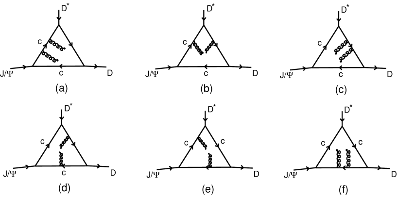
Figure 6: Gluon condensate diagrams contributing to the correlation function in Eq. (2).

In Fig. 8 we show the gluon condensate diagrams contributing to the correlation function in Eq. (2). We give bellow the expressions for all diagrams contribution in terms of $\Pi_{G}(t,M^{2},{M^{\prime}}^{2})$ appearing in Eq. (9).

$$\Pi_{G}^{(a)}(t,M^{2},{M^{\prime}}^{2})=-{{{M^{\prime}}}^{6}\over M^{2}(M^{2}+{M^{\prime}}^{2})^{2}}\int_{1/{M^{\prime}}^{2}}^{\infty}~{}d\alpha~{}e^{-{m_{c}^{2}\alpha(M^{2}+\alpha{{M^{\prime}}}^{4})\over M^{2}(\alpha{M^{\prime}}^{2}-1)}}~{}e^{t(\alpha{M^{\prime}}^{2}-1)\over M^{2}+{M^{\prime}}^{2}}\bigg{[}{1\over 2}+$$ (22)

$$- \left.{m_{c}^{2}\over 6}{\alpha(M^{2}+\alpha{{M^{\prime}}}^{4})\over M^{2}(\alpha{M^{\prime}}^{2}-1)}\right],$$

$$\Pi_{G}^{(b)}(t,M^{2},{M^{\prime}}^{2})=-{{M^{\prime}}^{2}\over 6M^{2}(M^{2}+{M^{\prime}}^{2})}\int_{1/{M^{\prime}}^{2}}^{\infty}~{}d\alpha~{}e^{-{m_{c}^{2}\alpha(M^{2}+\alpha{{M^{\prime}}}^{4})\over M^{2}(\alpha{M^{\prime}}^{2}-1)}}~{}e^{t(\alpha{M^{\prime}}^{2}-1)\over M^{2}+{M^{\prime}}^{2}}\bigg{[}\alpha t{M^{\prime}}^{2}+$$ (23)

$$+ {1\over\alpha{M^{\prime}}^{2}-1}\bigg{(}-{M^{\prime}}^{2}+2\alpha{{M^{\prime}}}^{4}-M^{2}(3-5\alpha{M^{\prime}}^{2}+\alpha^{2}{{M^{\prime}}}^{4})-m_{c}^{2}\alpha(M^{2}+{M^{\prime}}^{2}(2\alpha{M^{\prime}}^{2}+$$

$$- 1)+\alpha{M^{\prime}}^{2}\left({m_{c}^{2}\alpha^{2}{M^{\prime}}^{2}\over M^{2}}{(M^{2}(M^{2}+2{M^{\prime}}^{2})-\alpha{{M^{\prime}}}^{6}(\alpha{M^{\prime}}^{2}-2))\over(\alpha{M^{\prime}}^{2}-1)^{2}}+M^{2}+3\alpha{{M^{\prime}}}^{4}+\right.$$

$$+ \left.\left.\left.{t{M^{\prime}}^{2}(\alpha M^{2}+1)(M^{2}+\alpha{{M^{\prime}}}^{4})\over(M^{2}+{M^{\prime}}^{2})^{2}}+{{M^{\prime}}^{2}(M^{2}+\alpha{{M^{\prime}}}^{4})(2\alpha{M^{\prime}}^{2}+\alpha M^{2}-1))\over(M^{2}+{M^{\prime}}^{2})(\alpha{M^{\prime}}^{2}-1)}\right)\right)\right],$$

$$\Pi_{G}^{(c)}(t,M^{2},{M^{\prime}}^{2})=0,\;\;\;\mbox{ since it is proportional to }m_{q},$$ (24)

$$\Pi_{G}^{(d1)}(t,M^{2},{M^{\prime}}^{2})=-{{M^{\prime}}^{2}\over 6M^{2}}\int_{1/{M^{\prime}}^{2}}^{\infty}~{}d\alpha~{}e^{-{m_{c}^{2}\alpha(M^{2}+\alpha{{M^{\prime}}}^{4})\over M^{2}(\alpha{M^{\prime}}^{2}-1)}}~{}e^{t(\alpha{M^{\prime}}^{2}-1)\over M^{2}+{M^{\prime}}^{2}}{\alpha\over(\alpha{M^{\prime}}^{2}-1)}\bigg{[}$$ (25)

$$\left({m_{c}^{2}\alpha{M^{\prime}}^{2}\over 2}-{2(M^{2}+\alpha{{M^{\prime}}}^{4})\over\alpha{M^{\prime}}^{2}-1}\right)\left({m_{c}^{2}\alpha^{2}{M^{\prime}}^{2}(M^{2}-\alpha{{M^{\prime}}}^{4}+2{M^{\prime}}^{2})\over M^{2}(\alpha{M^{\prime}}^{2}-1)^{2}}+{t{M^{\prime}}^{2}(\alpha M^{2}+1)\over(M^{2}+{M^{\prime}}^{2})^{2}}\right)$$

$$+ {\alpha{M^{\prime}}^{2}\over 2(\alpha{M^{\prime}}^{2}-1)}\left({8(M^{2}+{M^{\prime}}^{2})\over\alpha{M^{\prime}}^{2}-1}-\alpha m_{c}^{2}{M^{\prime}}^{2}\right)\bigg{]},$$

$$\Pi_{G}^{(d2)}(t,M^{2},{M^{\prime}}^{2})={{{M^{\prime}}}^{4}\over 12M^{2}}\int_{1/{M^{\prime}}^{2}}^{\infty}~{}d\alpha~{}e^{-{m_{c}^{2}\alpha(M^{2}+\alpha{{M^{\prime}}}^{4})\over M^{2}(\alpha{M^{\prime}}^{2}-1)}}~{}e^{t(\alpha{M^{\prime}}^{2}-1)\over M^{2}+{M^{\prime}}^{2}}{\alpha^{2}\over(\alpha{M^{\prime}}^{2}-1)^{2}}\bigg{[}$$ (26)

$$\left({m_{c}^{2}\alpha^{2}{M^{\prime}}^{2}(M^{2}+{M^{\prime}}^{2})(M^{2}+2{M^{\prime}}^{2}-\alpha{{M^{\prime}}}^{4})\over M^{2}(\alpha{M^{\prime}}^{2}-1)^{2}}+{t{M^{\prime}}^{2}(\alpha M^{2}+1)\over(M^{2}+{M^{\prime}}^{2})}+\right.$$

$$- \left.{(M^{2}+2{M^{\prime}}^{2}+\alpha{{M^{\prime}}}^{2}M^{2})\over\alpha{M^{\prime}}^{2}-1}\right)\left({m_{c}^{2}\alpha^{2}{{M^{\prime}}}^{2}(M^{2}+2{M^{\prime}}^{2}-\alpha{{M^{\prime}}}^{4})\over M^{2}(\alpha{M^{\prime}}^{2}-1)^{2}}+{t{M^{\prime}}^{2}(\alpha M^{2}+1)\over(M^{2}+{M^{\prime}}^{2})^{2}}\right)+$$

$$+ {m_{c}^{2}\alpha^{2}{{M^{\prime}}}^{2}(M^{2}+{M^{\prime}}^{2})(\alpha{{M^{\prime}}}^{6}-\alpha{{M^{\prime}}}^{4}-3\alpha{M^{\prime}}^{2}M^{2}-4{M^{\prime}}^{2}-M^{2})\over M^{2}(\alpha{M^{\prime}}^{2}-1)^{3}}+{m_{c}^{2}\alpha^{2}{{M^{\prime}}}^{4}\over M^{2}}\bigg{(}$$

$$\left.{(M^{2}-\alpha{{M^{\prime}}}^{4}+2{M^{\prime}}^{2})\over(\alpha{M^{\prime}}^{2}-1)^{2}}\right)+{tM^{2}{M^{\prime}}^{2}(\alpha M^{2}+1)\over(M^{2}+{M^{\prime}}^{2})^{2}}-{2t\alpha{{M^{\prime}}}^{4}(\alpha M^{2}+1)\over(M^{2}+{M^{\prime}}^{2})(\alpha{M^{\prime}}^{2}-1)}+$$

$$+ \left.{{M^{\prime}}^{2}((\alpha M^{2}+2)(2\alpha{M^{\prime}}^{2}+1)+3\alpha M^{2})\over(\alpha{M^{\prime}}^{2}-1)^{2}}\right],$$

$$\Pi_{G}^{(d3)}(t,M^{2},{M^{\prime}}^{2})=-{{M^{\prime}}^{2}\over 3}\int_{1/{M^{\prime}}^{2}}^{\infty}~{}d\alpha~{}e^{-{m_{c}^{2}\alpha(M^{2}+\alpha{{M^{\prime}}}^{4})\over M^{2}(\alpha{M^{\prime}}^{2}-1)}}~{}e^{t(\alpha{M^{\prime}}^{2}-1)\over M^{2}+{M^{\prime}}^{2}}{\alpha\over(\alpha{M^{\prime}}^{2}-1)}\bigg{[}$$ (27)

$$- \left.1+{m_{c}^{2}\alpha^{2}{{M^{\prime}}}^{4}\over M^{2}(\alpha{M^{\prime}}^{2}-1)}-{tM^{2}(\alpha{M^{\prime}}^{2}-1)\over(M^{2}+{M^{\prime}}^{2})^{2}}\right],$$

$$\Pi_{G}^{(d4)}(t,M^{2},{M^{\prime}}^{2})={1\over 6M^{2}}\int_{1/{M^{\prime}}^{2}}^{\infty}~{}d\alpha~{}e^{-{m_{c}^{2}\alpha(M^{2}+\alpha{{M^{\prime}}}^{4})\over M^{2}(\alpha{M^{\prime}}^{2}-1)}}~{}e^{t(\alpha{M^{\prime}}^{2}-1)\over M^{2}+{M^{\prime}}^{2}}{1\over(\alpha{M^{\prime}}^{2}-1)}\bigg{[}$$ (28)

$$-{m_{c}^{4}\alpha^{2}(M^{2}+\alpha{{M^{\prime}}}^{4})\over 2(\alpha{M^{\prime}}^{2}-1)}+{t\alpha{M^{\prime}}^{2}(3M^{2}+{M^{\prime}}^{2}-\alpha M^{2}{M^{\prime}}^{2}+\alpha{{M^{\prime}}}^{4})\over(M^{2}+{M^{\prime}}^{2})}-{m_{c}^{2}t\alpha^{2}{{M^{\prime}}}^{2}\over 2}+$$

$$+ {1\over(M^{2}+{M^{\prime}}^{2})(\alpha{M^{\prime}}^{2}-1)}\bigg{(}M^{4}(-6+14\alpha{M^{\prime}}^{2}-9\alpha^{2}{{M^{\prime}}}^{4})+M^{2}{M^{\prime}}^{2}(-2+3\alpha{M^{\prime}}^{2}+$$

$$- 3\alpha^{2}{{M^{\prime}}}^{4})+{{M^{\prime}}}^{4}(-1-\alpha{M^{\prime}}^{2}+\alpha^{2}{{M^{\prime}}}^{4})++m_{c}^{2}\alpha({{M^{\prime}}}^{4}(1+4\alpha{M^{\prime}}^{2}-\alpha^{2}{{M^{\prime}}}^{4})+$$

$$+ 2M^{4}(-1+3\alpha{M^{\prime}}^{2})+M^{2}{M^{\prime}}^{2}(1+6\alpha{M^{\prime}}^{2}+\alpha^{2}{{M^{\prime}}}^{4}))\bigg{)}\bigg{]},$$

$$\Pi_{G}^{(d)}(t,M^{2},{M^{\prime}}^{2})=\Pi_{G}^{(d1)}+\Pi_{G}^{(d2)}+\Pi_{G}^{(d3)}+\Pi_{G}^{(d4)}$$ (29)

$$\Pi_{G}^{(e)}(t,M^{2},{M^{\prime}}^{2})=-{{{M^{\prime}}}^{2}\over 6M^{2}(M^{2}+{M^{\prime}}^{2})}\int_{1/{M^{\prime}}^{2}}^{\infty}~{}d\alpha~{}e^{-{m_{c}^{2}\alpha(M^{2}+\alpha{{M^{\prime}}}^{4})\over M^{2}(\alpha{M^{\prime}}^{2}-1)}}~{}e^{t(\alpha{M^{\prime}}^{2}-1)\over M^{2}+{M^{\prime}}^{2}}{M^{2}+\alpha{{M^{\prime}}}^{4}\over\alpha{M^{\prime}}^{2}-1},$$ (30)

$$\Pi_{G}^{(f)}(t,M^{2},{M^{\prime}}^{2})={{M^{\prime}}^{2}\over 6M^{2}}\int_{1/{M^{\prime}}^{2}}^{\infty}~{}d\alpha~{}e^{-{m_{c}^{2}\alpha(M^{2}+\alpha{{M^{\prime}}}^{4})\over M^{2}(\alpha{M^{\prime}}^{2}-1)}}~{}e^{t(\alpha{M^{\prime}}^{2}-1)\over M^{2}+{M^{\prime}}^{2}}{\alpha\over(\alpha{M^{\prime}}^{2}-1)^{2}}\bigg{[}$$ (31)

$${m_{c}^{2}\alpha(M^{2}+{M^{\prime}}^{2})^{2}\over M^{2}(\alpha{M^{\prime}}^{2}-1)}-2M^{2}-{M^{\prime}}^{2}-{m_{c}^{2}\alpha^{2}{{M^{\prime}}}^{4}(M^{2}+{M^{\prime}}^{2})\over M^{2}(\alpha{M^{\prime}}^{2}-1)}+{tM^{2}(\alpha{M^{\prime}}^{2}-1)\over(M^{2}+{M^{\prime}}^{2})}+$$

$$- -{m_{c}^{2}\alpha^{2}{{M^{\prime}}}^{2}(M^{2}+{M^{\prime}}^{2})(M^{2}+2{M^{\prime}}^{2}-\alpha{{M^{\prime}}}^{4})\over M^{2}(\alpha{M^{\prime}}^{2}-1)^{2}}-{t{M^{\prime}}^{2}(\alpha M^{2}+1)\over(M^{2}+{M^{\prime}}^{2})}+$$

$$+ \left.{2\alpha M^{2}{M^{\prime}}^{2}+{M^{\prime}}^{2}+\alpha{{M^{\prime}}}^{4}\over\alpha{M^{\prime}}^{2}-1}\right],$$

References

- (1) N. Isgur and M. Wise, Phys. Lett. B232, 113 (1989); B237, 527 (1990); G. Grinstein, Nucl. Phys. B339, 253 (1990); H. Georgi, Phys. Lett. B240, 447 (1990).
- (2) A. Deandrea, G. Nardulli and A.D. Polosa, Phys. Rev. D68, 034002 (2003).
- (3) Y. Oh, T. Song and S.H. Lee, Phys. Rev. C63, 034901 (2001); Y. Oh, T. Song, S.H. Lee and C.-Y. Wong, J.Korean Phys.Soc. 43, 1003 (2003).
- (4) F.S. Navarra, M. Nielsen and M.R. Robilotta, Phys. Rev. C64, 021901 (R) (2001).
- (5) K.L. Haglin and C. Gale, J.Phys. G30, S375 (2004).
- (6) F.S. Navarra, M. Nielsen, M.E. Bracco, M. Chiapparini and C.L. Schat, Phys. Lett. B489, 319 (2000).
- (7) F.S. Navarra, M. Nielsen, M.E. Bracco, Phys. Rev. D65, 037502 (2002).
- (8) M.E. Bracco, M. Chiapparini, A. Lozea, F.S. Navarra and M. Nielsen, Phys. Lett. B521, 1 (2001).
- (9) R.D. Matheus, F.S. Navarra, M. Nielsen and R. Rodrigues da Silva, Phys. Lett. B541, 265 (2002).
- (10) M.A. Shifman, A.I. Vainshtein and V.I. Zakharov, Nucl. Phys. B120, 316 (1977).
- (11) L.J. Reinders, H. Rubinstein and S. Yazaki, Phys. Rep. 127, 1 (1985).
- (12) B.L. Ioffe and A.V. Smilga, Nucl. Phys. B216 373 (1983); Phys. Lett. B114, 353 (1982).
- (13) R. Rodrigues da Silva, R.D. Matheus, F.S. Navarra, M. Nielsen, Braz.J.Phys. 34, 236 (2004).
- (14) Particle Data Group, K. Hagiwara et al., Phys. Rev. D66, 1 (2002).
- (15) V.M. Belyaev, V.M. Braun, A. Khodjamirian and R. Ruckl, Phys. Rev. D51, 6177 (1995).
- (16) Khodjamirian et al., Phys. Lett. B457, 245 (1999).