Radiative corrections to radiative $\pi e2$ decay

Abstract

The lowest order radiative corrections (RC) to width and spectra of radiative $\pi e2$ decay are calculated. We take into account virtual photon emission contribution as well as soft and hard real photon emission one. The result turns out to be consistent with the standard Drell-Yan picture for the width and spectra in the leading logarithmical approximation which permits us to generalize it to all orders of perturbation theory. Explicit expressions of nonleading contributions are obtained. The contribution of short distance is found to be in agreement with Standard Model predictions. It is presented as a general normalization factor. We check the validity of the Kinoshita-Lee-Nauenberg theorem about cancellation in the total width of the mass singularities at zero limit of electron mass. We discuss the results of the previous papers devoted to this problem. The Dalitz plot distribution is illustrated numerically.

I Introduction

The process of radiative negative pion decay

$$\pi^{-}(p)\to e^{-}(r)+\bar{\nu}_{e}(q)+\gamma(k)$$ (1)

attracts a lot of attention both experimentally and theoretically Bryman:et , Pocanic:2003tp , Bardin:ia , Nikitin , Komachenko:1992hr , Belyaev:1991gs , Poblaguev:2003ib . The main reason is a unique possibility to extract the so-called structure-dependent part $M_{SD}$ of the matrix element

$$M=M_{IB}+M_{SD},$$ (2)

which can be described in terms of vector and axial-vector formfactors of the pion and the hints of a ”new physics” including a possible revealing of tensor forces (which are absent in the traditional Standard Model).

Due to the numerical smallness of $M_{SD}$ compared to the inner bremsstrahlung part $M_{IB}$, the problem of taking into account radiative corrections (RC) becomes essential. The lowest order RC for a special experimental set-up was calculated in 1991 in Nikitin , where, unfortunately, the contribution to RC from emission of an additional hard photon was not considered. This is the motivation of our paper.

Our paper is organized as follows. In part II, we calculate the contributions to RC from emission of virtual photons (at 1 loop level) and the ones arising from additional soft photon emission. For definiteness, we consider RC to the QED-part of the matrix element $M_{IB}$

$$M_{IB}=-iA~{}\bar{u}_{e}(r)\left[\frac{(\varepsilon^{*}r)}{(kr)}-\frac{(\varepsilon^{*}p)}{(kp)}+\frac{\hat{\varepsilon}^{*}\hat{k}}{2(kr)}\right](1+\gamma_{5})v_{\nu}(q),\qquad A=e\frac{G_{F}}{\sqrt{2}}V_{ud}f_{\pi}m,$$ (3)

where $e=\sqrt{4\pi\alpha}$, $G_{F}=1.17\cdot 10^{-5}~{}GeV^{-2}$ is the Fermi coupling constant, $\varepsilon$ is the photon polarization vector, $f_{\pi}=131~{}MeV$ is the pion decay constant, $V_{ud}$ is the element of the Cabbibo-Kobayashi-Maskawa quark mixing matrix, and $M$ and $m$ are masses of pion and electron. The explicit form of the matrix element including $M_{SD}$ is given in Appendix A.

In part III, we consider the process of double radiative pion decay and extract the leading contribution proportional to ”large” logarithm $\ln M^{2}/m^{2}$ which arises from the kinematics of emission of one of the hard photons collinearly to electron momentum. We arrive at the result which can be obtained by applying the quasireal electron method BFK .

In conclusion, we combine the leading contributions and find that the result can be expressed in terms of the electron structure function Kuraev:hb . Really, the lowest order RC in the leading logarithmical approximation (LLA) (i.e., keeping terms $\left(\frac{\alpha}{\pi}\ln\frac{M^{2}}{m^{2}}\right)^{n}$) turns out to reproduce two first order contribution of the electron structure function obeying the evolution equation of renormalization group (RG). This fact permits us to generalize our result to include higher orders of perturbation theory (PT) contributions to the electron structure function in the leading approximation. In conclusion, we also argue that our consideration can be generalized to the whole matrix element.

As for the next-to-leading contributions, we put them in the form of the so-called $K$-factor which collects all the non-enhanced (by large logarithm) contributions. Part of them, arising from virtual and real soft photon emission, is given analytically. The other part, arising from emission of additional hard photon in noncollinear kinematics is presented in Appendix C in terms of 3-fold convergent integrals.

In Appendix B, we give the simplified form of RC (the lowest order ones) and make an estimation of the omitted terms which determine the accuracy of the simplified RC.

Appendix D contains the list of 1-loop integrals used in calculation of 1-loop Feynman integrals.

In tables 3, 3, 3 the result of numerical calculation of contributions of RC to Dalitz-plot distribution in Born level, leading and non-leading approximations are given.

II Virtual and soft real photon emission RC

A rather detailed calculation of the lowest order RC was carried out in Nikitin . Nonclear manipulations with a soft photon emission contribution used in Nikitin results in a wrong form of the dependence of RC on the photon detection threshold $\Delta\varepsilon$ which contradicts the general theorem Yennie:ad . Another reason for our revision of Nikitin is the mixing of (on-mass shell and dimensional) regularization schemes in it. We use here the unrenormalized theory with the ultraviolet cut-off parameter $\Lambda$.

Following Nikitin , we first consider RC to the ”largest” contribution – inner bremsstrahlung $M_{IB}$. As well we consider the central part of Dalitz-plot and omit (if possible) $\beta\equiv\left(\frac{m}{M}\right)^{2}=1.34\cdot 10^{-5}$, that is $\beta\rightarrow 0$.

We distinguish the contribution to RC from emission of virtual and soft additional photons ($\Delta_{V}$ and $\Delta_{S}$, respectively):

$$\sum_{spin~{}states}\left.\left|M_{IB}\right|^{2}\right|_{virt+soft}=\sum\left|M_{IB}\right|^{2}\left(1+\frac{\alpha}{\pi}\left(\Delta_{V}+\Delta_{S}\right)\right),$$ (4)

where

$$\sum\left|M_{IB}\right|^{2}=8A^{2}\frac{(1-y)(1+(1-x)^{2})}{x^{2}(x+y-1)}\equiv 8A^{2}B(x,y),$$ (5)

(here $x=\frac{2(kp)}{M^{2}}$, $y=\frac{2(rp)}{M^{2}}$, $z=\frac{2(kr)}{M^{2}}$, $M$ is the pion mass).

Soft photon emission RC have a standard form (see, for example Bytev:2002nx , formula (16))

$$\frac{\alpha}{\pi}\Delta_{S} = -\frac{\alpha}{2\pi^{2}}\int\frac{d^{3}k_{1}}{2\omega_{1}}\left.\left(\frac{p}{(k_{1}p)}-\frac{r}{(k_{1}r)}\right)^{2}\right|_{\omega_{1}=\sqrt{{\vec{k}_{1}}^{2}+\lambda^{2}}<\Delta\varepsilon\ll yM}=$$ (6)

$$= \frac{\alpha}{\pi}\left[\left(L_{e}-2\right)\ln\left(\frac{2\Delta\varepsilon}{\lambda}\right)+\frac{1}{2}L_{e}-\frac{1}{4}L_{e}^{2}+1-\xi_{2}\right]\left(1+O(\beta)\right),$$

where $k_{1}$ the additional soft photon momentum, $L_{e}=\ln\frac{y^{2}}{\beta}$ and $\lambda$ is the ”photon mass”, $\xi_{2}=\frac{\pi^{2}}{6}$. This result agrees with the general analysis of infrared behavior given in Yennie:ad .

Now let us consider the calculation of the virtual photon emission corrections. First, we use the minimal form for introduction of the electromagnetic field through the generalization of the derivative $p_{\mu}\rightarrow p_{\mu}-ieA_{\mu}$.

The sum of contributions (all particles except antineutrino can be on or off mass shell) leads to:

$$\frac{\hat{\varepsilon}(\hat{r}+\hat{k}+m)\hat{p}}{(r+k)^{2}-m^{2}}v_{\nu}(q)-\hat{\varepsilon}v_{\nu}(q)=m\cdot\frac{\hat{\varepsilon}(\hat{r}+\hat{k}+m)}{(r+k)^{2}-m^{2}}v_{\nu}(q),$$ (7)

$p=r+k+q$. Thus, we can extract the contact photon emission vertex and obtain the effective vertex $\sim m$, as it is shown in Fig. 1.

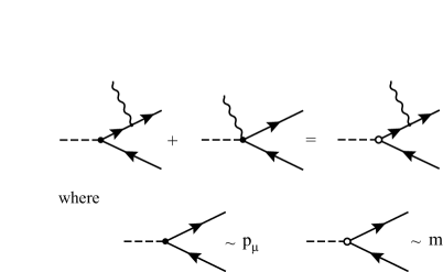
Figure 1: Effective vertex.

In terms of this new effective vertex we can write down the 1-loop Feynman diagrams (FD) of virtual photon emission RC ($\frac{\alpha}{\pi}\Delta_{V}$) which are shown in Fig. 2 (see Nikitin ). We should notice that these diagrams can be separated out into four classes. The contributions of each of these classes are gauge invariant.

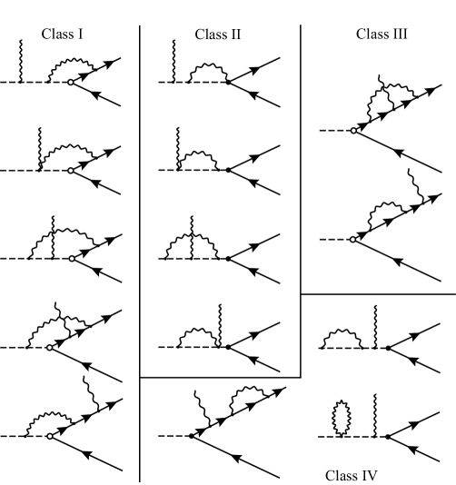
Figure 2: Feynman diagrams of virtual contributions.

Three first classes were considered in Nikitin , where their gauge invariance and in particular zero contribution of class II were strictly shown. The last statement directly follows from the gauge-invariance.

The contribution of class III contains the regularized mass and vertex operators. The relevant matrix element has the form:

$$M_{III}=-iA\frac{\alpha}{2\pi M}\bar{u}_{e}(r)\left[\left(\hat{\varepsilon}^{*}-\hat{k}\frac{(\varepsilon^{*}r)}{(kr)}\right)B_{1}+\frac{\hat{k}\hat{\varepsilon}^{*}}{M}B_{2}\right](1+\gamma_{5})v_{\nu}(q),$$ (8)

where

$$B_{1} = \frac{1}{\sqrt{\beta}}\frac{1}{2a}\left(1-\frac{y^{\prime}}{a}l_{S}\right),$$

$$B_{2} = \frac{1}{\beta}\left[\frac{1}{y^{\prime}}n+\frac{1}{2a}-\frac{2y^{\prime 2}+3y^{\prime}+2}{2y^{\prime}a^{2}}l_{S}\right],$$

$$n = \frac{1}{y^{\prime}}\left[Li_{2}(1)-Li_{2}(1+y^{\prime})-i\pi\ln(1+y^{\prime})\right],$$

here $l_{S}=\ln\frac{z}{\beta}-i\pi$,  $a=1+y^{\prime}$,  $y^{\prime}=\frac{2(kr)}{m^{2}}$. We see that $M_{III}$ is explicitly gauge-invariant and is free from infrared singularities. At the realistic limit $y\sim x\sim z\gg\beta$ (rather far from the boundaries of Dalitz-plot) we obtain for contribution to the matrix element square (structure $\sim B_{1}$ gives a zero contribution in the limit $\beta\to 0$) (in agreement with Nikitin ):

$$\Delta\left|M_{III}\right|^{2}=2Re\left\{\left(M_{IB}\right)^{+}M_{III}\right\}=-\frac{8\alpha}{\pi}A^{2}\frac{1-y}{xz}\left(\frac{1}{2}-\ln\left(\frac{z}{\beta}\right)\right).$$ (9)

As we work within the unrenormalized theory, we should consider class IV (not considered in Nikitin ) which concerns the contribution of counter-terms due to renormalization of the pion and electron wave functions (see Bytev:2002nx , formula (17))

$$\Delta\left|M_{IV}\right|^{2}=\sum\left|M_{IB}\right|^{2}\cdot\frac{\alpha}{2\pi}\left\{\left[-\frac{1}{2}L_{\Lambda}+\frac{3}{2}\ln\beta+\ln\frac{M^{2}}{\lambda^{2}}-\frac{9}{4}\right]+\left[L_{\Lambda}+\ln\frac{M^{2}}{\lambda^{2}}-\frac{3}{4}\right]\right\},$$ (10)

where $L_{\Lambda}=\ln\frac{\Lambda^{2}}{M^{2}}$ and $\Lambda$ is the ultraviolet cut-off parameter to be specified later. The first term in the brackets in the r.h.s. is the electron wave function renormalization constant and the second one corresponds to the pion wave function renormalization.

Let now consider the contributions of FDs of class I. In Nikitin the explicit gauge-invariance of the sum was demonstrated: $k_{\mu}\left(T_{1}^{\mu}+T_{2}^{\mu}+T_{3}^{\mu}+T_{4}^{\mu}+T_{5}^{\mu}\right)=0$, where $T_{i}^{\mu}$ is the contribution of the corresponding FD of Class I (see in Fig. 2).

The contribution to the matrix element square can be written as:

$$\Delta\left|M_{I}\right|^{2}=2Re\left\{\left(M_{IB}\right)^{+}M_{I}\right\}=\frac{\alpha}{2\pi}A^{2}Re\left\{\int\frac{d^{4}k_{1}}{i\pi^{2}}\left[A_{1}+A_{2}+A_{3}+A_{4}+A_{5}\right]\right\},$$ (11)

where

$$A_{1} = \frac{2}{x}\cdot\frac{1}{(0)(1^{\prime})(2)}Sp~{}[\hat{r}(2(\hat{p}-\hat{k})-\hat{k}_{1})(\hat{r}-\hat{k}_{1})(1+\gamma_{5})\hat{q}\left((Qp)+\frac{\hat{k}\hat{p}}{z}\right)]\frac{1}{M^{2}},$$

$$A_{2} = \frac{2}{(0)(1^{\prime})(2)}Sp~{}[\hat{r}\gamma_{\lambda}(\hat{r}-\hat{k}_{1})(1+\gamma_{5})\hat{q}\left(Q^{\lambda}+\frac{\hat{k}\gamma^{\lambda}}{z}\right)],$$

$$A_{3} = -\frac{2}{(0)(1)(1^{\prime})(2)}Sp~{}[\hat{r}(2\hat{p}-\hat{k}_{1})(\hat{r}-\hat{k}_{1})(1+\gamma_{5})\hat{q}\left((Q(p-k_{1}))+\frac{\hat{k}(\hat{p}-\hat{k}_{1})}{z}\right)],$$

$$A_{4} = -\frac{1}{(0)(1)(2)(2^{\prime})}Sp~{}[\hat{r}(2\hat{p}-\hat{k}_{1})(\hat{r}-\hat{k}_{1})\gamma_{\lambda}(\hat{r}+\hat{k}-\hat{k}_{1})(1+\gamma_{5})\hat{q}\left(Q^{\lambda}+\frac{\hat{k}\gamma^{\lambda}}{z}\right)],$$

$$A_{5} = -\frac{1}{z}\frac{1}{(0)(1)(2^{\prime})}Sp~{}[\hat{r}\gamma_{\lambda}(\hat{r}+\hat{k})(2\hat{p}-\hat{k}_{1})(\hat{r}+\hat{k}-\hat{k}_{1})(1+\gamma_{5})\hat{q}\left(Q^{\lambda}+\frac{\hat{k}\gamma^{\lambda}}{z}\right)]\frac{1}{M^{2}}.$$

where $k_{1}$ virtual photon momentum, $Q_{\mu}=-\frac{p_{\mu}}{(kp)}+\frac{r_{\mu}}{(kr)}=\frac{2}{M^{2}}\left(\frac{r_{\mu}}{z}-\frac{p_{\mu}}{x}\right)$. Here the denominators of the pion and electron Green functions $(i)$ are listed in Appendix D. We omitted $m$ everywhere in the numerators. The ultraviolet divergences are present in $A_{1}$ and $A_{5}$.

Using the set of vector and scalar integrals listed in Appendix D and adding the soft photon emission corrections we obtain

$$1+\frac{\alpha}{\pi}\left(\Delta_{V}+\Delta_{S}\right)=$$

$$\qquad=S_{W}\left\{1+\frac{\alpha}{\pi}\left[\left(L_{e}-1\right)\left(\ln\Delta+\frac{3}{4}\right)-\ln\Delta+\frac{1}{B^{\prime}(x,y)}\cdot R(x,y)\right]\right\},$$ (12)

where $S_{W}=1+\frac{3}{4}\frac{\alpha}{\pi}L_{\Lambda}$, $\Delta\equiv\frac{2\Delta\varepsilon}{yM}$. $R(x,y)$ looks like

$$R(x,y) = 4ab\bar{y}\left(-5\ln y+\frac{3}{2}-4\ln y\ln\frac{2}{y}\right)-$$ (13)

$$- 8b\ln y\left(-a\bar{y}(1+\ln 4)+((x-2)^{2}-y(a+2))\ln x+x(1+y^{2})\ln z\right)+$$

$$+ 2b\ln^{2}y\left(-16\bar{y}+x(16-7x+7y(x-2))\right)-$$

$$- \xi_{2}\cdot 8b\bar{y}(6+2x^{2}-x(5+y))+$$

$$+ 4x\bar{y}zb\left(Li_{2}\left(\frac{y-1}{y}\right)-Li_{2}(1-y)\right)+8ab\bar{y}Li_{2}(x)+$$

$$+ 8ab\bar{y}\ln x\ln(1-x)-8x\bar{x}\bar{y}z(x+y-2)\ln z-$$

$$- 4x\bar{y}z\ln^{2}z(-\bar{x}+y(x-2)+y^{2})-4x\bar{y}b,$$

$$B^{\prime}(x,y) = 8(1-y)(1+(1-x)^{2})(x+y-2)^{2}=8ab\bar{y},$$ (14)

where $a=1+(1-x)^{2}$, $b=(x+y-2)^{2}$, $\bar{x}=1-x$, $\bar{y}=1-y$, $z=x+y-1$. Here we do not have a complete agreement with the result of Nikitin . Note that the sum $\Delta_{S}+\Delta_{V}$ does not depend on ”photon mass” $\lambda$, and, besides, the coefficient at large logarithm $L_{e}$ agrees with RG predictions.

III Emission of additional hard photon

Emission of additional hard photon (not considered in the previous papers concerning RC to the $\pi\to e\nu\gamma$ decay), i.e., the process of double photon emission in the $\pi e2$ decay: $\pi^{-}(p)\rightarrow e^{-}(r)+\bar{\nu}_{e}(q)+\gamma(k_{1})+\gamma(k_{2})$ is described by 11 FD drawn in Fig. 3.

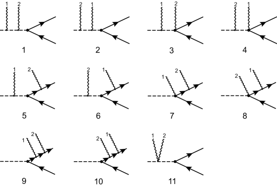
Figure 3: Feynman diagrams, describing the double radiative pion decay.

In collinear kinematics (when one of the real photons is emitted close to the electron emission direction) the relevant contribution to the differential width contains large logarithms.

The matrix element of the double radiative pion decay has the form

$$M^{\pi\rightarrow e\nu\gamma\gamma} = iA\sqrt{4\pi\alpha}~{}\left[\bar{u}_{e}(r)O_{\mu\nu}(1+\gamma_{5})v_{\nu}(q)\right]\cdot\varepsilon_{1}^{\mu}(k_{1})\varepsilon_{2}^{\nu}(k_{2}),$$ (15)

where $\varepsilon_{1,2}$ are the photons polarization vectors which obey the Lorentz condition: $(k_{1}~{}\varepsilon_{1}(k_{1}))=(k_{2}~{}\varepsilon_{2}(k_{2}))=0$. The tensor $O^{\mu\nu}$ has the form

$$O^{\mu\nu} = \left(-2g^{\mu\nu}+\frac{2p^{\mu}\cdot 2(p-k_{1})^{\nu}}{-2(k_{1}p)}+\frac{2p^{\nu}\cdot 2(p-k_{2})^{\mu}}{-2(k_{2}p)}\right)\frac{1}{(p-k_{1}-k_{2})^{2}-M^{2}}+$$ (16)

$$+ \frac{2p^{\mu}}{-2(k_{1}p)}\frac{\gamma^{\nu}(\hat{r}+\hat{k}_{2}+m)}{2(k_{2}r)}+\frac{2p^{\nu}}{-2(k_{2}p)}\frac{\gamma^{\mu}(\hat{r}+\hat{k}_{1}+m)}{2(k_{1}r)}+$$

$$+ \left[\gamma^{\nu}\frac{\hat{r}+\hat{k}_{2}+m}{2(k_{2}r)}\gamma^{\mu}+\gamma^{\mu}\frac{\hat{r}+\hat{k}_{1}+m}{2(k_{1}r)}\gamma^{\nu}\right]\frac{\hat{r}+\hat{k}_{1}+\hat{k}_{2}+m}{(r+k_{1}+k_{2})^{2}-m^{2}}.$$

One can be convinced in the explicit fulfillment of the requirements of Bose-symmetry and gauge-invariance $M^{\pi\rightarrow e\nu\gamma\gamma}(\varepsilon_{1}\rightarrow k_{1})=M^{\pi\rightarrow e\nu\gamma\gamma}(\varepsilon_{2}\rightarrow k_{2})=0$. The expression for $\sum\left|M^{\pi\rightarrow e\nu\gamma\gamma}\right|^{2}\sim Sp\left[(\hat{r}+m)O^{\mu\nu}\hat{q}~{}O_{\mu\nu}\right]$ is rather cumbersome.

The contribution to the differential width has the form

$$d\Gamma^{hard}_{IB}=\frac{1}{2M}\sum\left|M^{\pi\rightarrow e\nu\gamma\gamma}\right|^{2}d\Phi_{4},$$ (17)

$$d\Phi_{4}=\frac{(2\pi)^{4}}{(2\pi)^{12}}\frac{d^{3}q}{2q_{0}}\frac{d^{3}r}{2r_{0}}\frac{d^{3}k_{1}}{2\omega_{1}}\frac{d^{3}k_{2}}{2\omega_{2}}~{}\delta^{4}(p-q-r-k_{1}-k_{2}).$$ (18)

We do not take into account the identity of photons: we believe the photon with momentum $k_{1}$ to be a measurable one with $\frac{2(k_{1}p)}{M^{2}}=x$ and the photon with momentum $k_{2}$ to be a background one with $\frac{2(k_{2}p)}{M^{2}}>\Delta$ and most general kinematics.

It is convenient to consider separately the collinear kinematics of emission of one of the photons, i.e., the case when the angle of emission of one of the final photon direction of motion is rather small $\theta_{i}=(\widehat{\vec{r},\vec{k}_{i}})<\theta_{0}\ll 1$, $\theta_{0}^{2}\gg\beta$. (Note that double collinear kinematics is excluded since the invariants $x^{\prime}_{1,2}=\frac{2(k_{1,2}r)}{M^{2}}$ cannot be small simultaneously).

The contribution of these collinear kinematics to the differential width contains ”large logarithms” $L_{e}$. To extract the relevant contribution we can use the quasireal electron method BFK . For this aim let us arrange the integration over phase volume in the following way:

$$\left|M\right|^{2}d\Phi_{4}=\left|M_{C}\right|^{2}d\Phi_{4}^{C}+\left|M_{C}\right|^{2}(d\Phi_{4}-d\Phi_{4}^{C})+\left(\left|M\right|^{2}-\left|M_{C}\right|^{2}\right)d\Phi_{4},$$ (19)

with

$$(4\pi\alpha)^{-2}\sum\left|M_{C}\right|^{2}=\left[\frac{8}{x^{\prime}_{2}}\frac{y^{2}+(y+x_{2})^{2}}{x_{2}(x_{2}+y)}-\frac{16\beta}{{x^{\prime}_{2}}^{2}}\right]\cdot\frac{(1+(1-x_{1})^{2})(1-x_{2}-y)}{x_{1}^{2}(x_{1}+x_{2}+y-1)},$$ (20)

$$(2\pi)^{8}M^{-4}d\Phi_{4} = M^{-4}\frac{d^{3}r~{}d^{3}k_{1}~{}d^{3}k_{2}}{2r_{0}~{}2\omega_{1}~{}2\omega_{2}}~{}\delta\left(\left(p-r-k_{1}-k_{2}\right)^{2}\right)=$$ (21)

$$= \frac{\pi^{2}}{2^{6}}~{}x_{1}x_{2}y~{}dx_{1}dx_{2}dy~{}dC_{1}~{}d\Omega_{2}~{}\times$$

$$\times \delta\left(1-x_{1}-x_{2}-y+\frac{x_{1}x_{2}}{2}(1-C_{12})+\frac{x_{1}y}{2}(1-C_{1})+\frac{x_{2}y}{2}(1-C_{2})\right),$$

$$(2\pi)^{8}M^{-4}d\Phi_{4}^{C} = \frac{\pi^{2}}{2^{5}}~{}\frac{x_{2}y}{y+x_{2}}dx_{1}dx_{2}dy~{}d\Omega_{2}^{C},$$ (22)

where $x_{1,2}=\frac{2(k_{1,2}p)}{M^{2}}$, $x^{\prime}_{1,2}=\frac{2(k_{1,2}r)}{M^{2}}$,  $C_{12}=\cos(\widehat{\vec{k}_{1},\vec{k}_{2}})$,  $C_{1,2}=\cos(\widehat{\vec{k}_{1,2},\vec{r}})$, $d\Omega_{2}$ is the angular phase volume of the photon with 4-momentum $k_{2}$.

Note that integration over the angular phase volume $d\Omega_{2}$ in $d\Phi_{4}^{C}$ (see (19)) is restricted by $\int d\Omega_{2}^{C}=\int\limits_{0}^{2\pi}d\phi\int\limits_{1-\theta_{0}^{2}/2}^{1}dC_{2}$ and in the second term in (19) $d\Phi_{4}-d\Phi_{4}^{C}$ can be replaced by $d\Phi_{4}$ with $\int d\Omega_{2}=\int\limits_{0}^{2\pi}d\phi\int\limits_{-1}^{1-\theta_{0}^{2}/2}dC_{2}$. The second and the third terms in (19) do not contain collinear singularities, i.e., are finite in the limit $\beta\rightarrow 0$.

The contribution of hard photon emission can be written out in the form

$$\frac{d\Gamma^{hard}_{IB}}{dxdy} = A^{2}\frac{\alpha}{2\pi}\int\limits_{y}^{1}\frac{dt}{t}B(x,t)\left[P_{\theta}^{(1)}\left(\frac{y}{t}\right)\left(L_{e}-1+\ln\frac{\theta_{0}^{2}}{4}\right)+1-\frac{y}{t}\right]+$$ (23)

$$+ \frac{\alpha}{\pi}K^{hard}_{IB}(x,y,\theta_{0},\Delta),$$

where the function $B(x,t)$ is defined in (5),

$$P_{\theta}^{(1)}(z)=\frac{1+z^{2}}{1-z}\theta\left(1-z-\Delta\right),$$ (24)

and $K^{hard}_{IB}(x,y,\theta_{0},\Delta)$ represents the contribution of two last terms in (19). Now it is convenient to introduce the following quantity:

$$K^{h}_{IB}(x,y,\Delta)=K^{hard}_{IB}(x,y,\theta_{0},\Delta)+\int\limits_{y}^{1}\frac{dt}{t}B(x,t)\left[P_{\theta}^{(1)}\left(\frac{y}{t}\right)\ln\frac{\theta_{0}^{2}}{4}+1-\frac{y}{t}\right],$$ (25)

which does not already depend on the parameter $\theta_{0}$. The explicit view of $K^{h}_{IB}(x,y,\Delta)$ is given in Appendix C.

In the total sum of virtual, soft, and hard photon emission contributions all the auxiliary parameters – ”photon mass” $\lambda$ and $\Delta$ – are cancelled out. The resulting expression for the differential width with RC up to any order of QED PT with the leading logarithm $\frac{\alpha}{\pi}L_{e}\sim 1$ and the next-to-leading accuracy have the form

$$\frac{d\Gamma^{RC}_{IB}}{dxdy}=A^{2}S_{W}\int\limits_{y}^{1}\frac{dt}{t}B(x,t)D\left(\frac{y}{t}\right)\left(1+\frac{\alpha}{2\pi}K_{IB}(x,y)\right),$$ (26)

where $D(z)$ is the well-known electron structure function, which has the form

$$D(z)=\delta(1-z)+\frac{\alpha}{2\pi}\left(L_{e}-1\right)P^{(1)}(z)+\frac{1}{2!}\left(\frac{\alpha}{2\pi}\right)^{2}\left(L_{e}-1\right)^{2}P^{(2)}(z)+\cdots,$$ (27)

where

$$P^{(1)}=\lim_{\Delta\rightarrow 0}\left[\frac{1+z^{2}}{1-z}\theta(1-z-\Delta)+\delta(1-z)\left(2\ln\Delta+\frac{3}{2}\right)\right]=\left(\frac{1+z^{2}}{1-z}\right)_{+},$$ (28)

$$P^{(n)}(z)=\int\limits_{z}^{1}\frac{dt}{t}P^{(1)}(z)P^{(n-1)}\left(\frac{z}{t}\right).$$ (29)

The function $K_{IB}(x,y)$ is the so-called K-factor which here has the form

$$K_{IB}(x,y)=2\frac{R(x,y)}{B^{\prime}(x,y)}-2\ln\Delta+K^{h}_{IB}(x,y,\Delta),$$ (30)

where $R(x,y)$ and $B^{\prime}(x,y)$ was defined in (13) and (14). The quantity $K^{h}_{IB}(x,y,\Delta)-2\ln\Delta$ is finite at $\Delta\to 0$ and its explicit expression is given in Appendix C.

IV Discussion

It is easy to see that in the total decay width all the dependence on $\beta$ disappears in accordance with the Kinoshita-Lee-Nauenberg (KLN) theorem KLN . Really, we obtain integrating over $y$:

$$\int\limits_{0}^{1}dy\int\limits_{y}^{1}\frac{dt}{t}D\left(\frac{y}{t}\right)\cdot f(t)=\int\limits_{0}^{1}dt~{}f(t)\int\limits_{0}^{t}\frac{dy}{t}D\left(\frac{y}{t}\right)=\int\limits_{0}^{1}dt~{}f(t)\int\limits_{0}^{1}dzD\left(z\right)=\int\limits_{0}^{1}dtf(t).$$ (31)

Now let us discuss the dependence on the ultraviolet cut-off $\Lambda$. It was shown in a series of remarkable papers by A. Sirlin Sirlin:cs that the Standard Model provides $\Lambda=M_{W}$. Another important moment (not considered here) is the evolution with respect to ultraviolet scale of virtual photon momenta from hadron scale ($m_{\rho}$) up to $M_{Z}$ Sirlin:cs . It results in effective replacement $S_{W}\rightarrow S_{EW}=1+\frac{\alpha}{\pi}\ln\frac{M_{Z}^{2}}{m_{\rho}^{2}}\approx 1.0232.$ So all the QED corrections to the total width are small $\sim O\left(\frac{\alpha}{\pi}\right)$, but the electroweak ones rather large: $\Gamma\approx\Gamma_{0}\cdot S_{EW}$. The factor $S_{EW}$ can be absorbed by pion life-time constant $f_{\pi}\sqrt{S_{EW}}\to f_{\pi}^{exp}$ Holstein:ua . Thus, we replace $A$, defined in (3), with $A_{exp.}$

$$A=e\frac{G_{F}}{\sqrt{2}}V_{ud}f_{\pi}m\quad\to\quad A_{exp.}=e\frac{G_{F}}{\sqrt{2}}V_{ud}f_{\pi}^{exp}m.$$ (32)

We also note here that according to Holstein:ua we must use the redefined constant $A_{exp.}$ in the Born approximation. That is why we use $A_{exp.}$ in Appendix A.

In our explicit calculations we considered RC to the inner bremsstrahlung part of the matrix element. Let us now argue that in the integrand of the r.h.s. of (26) one can replace $B(x,y)$ by the total value including the structure dependent contribution $\Phi_{tot}^{(0)}(x,y)$ which is defined in Appendix A in (38). This fact can be proved in the leading logarithmic approximation. One of contributions arising from additional hard photon emission close to the electron direction can be obtained by applying the quasireal electron method BFK and has the form (26) with $P^{(1)}\rightarrow P^{(1)}_{\theta}$. The KLN theorem in a unique form provides the soft photon emission and virtual RC to be of a form with complete kernel $P(z)$ in the structure function $D(z)$ in (26). So our result reads

$$\frac{d\Gamma_{RC}}{dxdy}=A_{exp.}^{2}\int\limits_{y}^{1}\frac{dt}{t}\Phi_{tot}^{(0)}(x,t)D\left(\frac{y}{t}\right)\left(1+\frac{\alpha}{2\pi}K(x,y)\right).$$ (33)

We also calculate the RC to the SD part in leading logarithmical approximation. Formula (33) can be trusted in the region where the IB part dominates. In the region where IB $\leq$ SD, which is suitable for SD measurement, both IB and SD are small; so the question about non-leading contributions becomes academical. Thus, we suggest here that K-factor is the same order of magnitude as for the IB part (i.e. $K(x,y)=K_{IB}(x,y)$), where it can be calculated in the model-independent way. Its numerical value is given in Table 3.

We underline that the explicit dependence on ”large logarithm” $L_{e}=\ln\frac{y^{2}}{\beta}$ is present in the Dalitz-plot distribution.

Now let us discuss the results obtained in some previous papers devoted to RC in the radiative pion decay.

In Nikitin , the hard photon emission was not considered which led to violation of the KLN-theorem.

In Komachenko:1992hr , Belyaev:1991gs , the main attention was paid to possible sources of tensor forces. As for real QED+EW corrections depicted in formula (13) in Komachenko:1992hr : $\frac{\delta\Gamma}{\Gamma}\approx 0.7\frac{\alpha}{\pi}\sim 0.2\%$ the QED leading RC was presumably omitted.

V Acknowledgements

We are grateful to RFFI grant 03-02 N 17077 for support. One of us (E.K.) is grateful to INTAS grants 97-30494 and 00366. We are also grateful to M. V. Chizhov for discussions and pointing out reference Poblaguev:2003ib . Besides, we are grateful to Paul Scherrer Institute (Villigen, Switzerland) for warm hospitality where the final part of this work was completed.

Appendix A Born amplitude

The radiative pion decay matrix element in the Born approximation has the form Poblaguev:2003ib

$$M=M_{IB}+M_{SD}+M_{T},$$ (34)

where

$$M_{IB} = -iA_{exp.}~{}\bar{u}_{e}(r)\left[\frac{(\varepsilon^{*}r)}{(kr)}-\frac{(\varepsilon^{*}p)}{(kp)}+\frac{\hat{\varepsilon}^{*}\hat{k}}{2(kr)}\right](1+\gamma_{5})v_{\nu}(q),$$ (35)

$$M_{SD} = \frac{A_{exp.}}{mMf_{\pi}^{exp.}}~{}\bar{u}_{e}(r)\gamma_{\mu}(1+\gamma_{5})v_{\nu}(q)~{}e_{\nu}\left[F_{V}~{}\varepsilon^{\mu\nu\alpha\beta}p_{\alpha}k_{\beta}+iF_{A}\left(g^{\mu\nu}(kp)-p^{\mu}k^{\nu}\right)\right],$$ (36)

$$M_{T} = -i\frac{A_{exp.}}{mf_{\pi}^{exp.}}~{}F_{T}~{}e^{\mu}k^{\nu}~{}\bar{u}_{e}(r)\sigma_{\mu\nu}(1+\gamma_{5})v_{\nu}(q)-$$ (37)

$$-i\frac{A_{exp.}}{mf_{\pi}^{exp.}}~{}F^{\prime}_{T}~{}(k_{\alpha}e_{\beta}-k_{\beta}e_{\alpha})\frac{Q^{\beta}Q_{\nu}}{Q^{2}}~{}\bar{u}_{e}(r)\sigma^{\alpha\nu}(1+\gamma_{5})v_{\nu}(q),$$

where $Q=p-k$. The constant $A_{exp.}$ defined in (32). Squaring amplitude (34) and summing over final photon polarizations leads to the following decay width:

$$\frac{d^{2}\Gamma^{0}}{dx~{}dy} = \Phi_{tot}^{(0)}(x,y)=\frac{M}{(2\pi)^{4}}A_{exp.}^{2}\frac{\pi}{2}\left\{\Phi_{IB}^{(0)}+\left(f_{V}+f_{A}\right)^{2}\Phi_{+}^{(0)}+\left(f_{V}-f_{A}\right)^{2}\Phi_{-}^{(0)}+\right.$$ (38)

$$\qquad\qquad\qquad+2\sqrt{\beta}\left(\left(f_{V}+f_{A}\right)\Phi_{Int+}^{(0)}+\left(f_{V}-f_{A}\right)\Phi_{Int-}^{(0)}\right)+$$

$$\qquad\qquad\qquad+\left.2\left(2f_{T}(f_{T}-f^{\prime}_{T})+f_{T}^{\prime 2}\right)\Phi_{T_{1}}^{(0)}+2\left(2(f_{T}-f^{\prime}_{T})+f_{T}^{\prime}x\right)\Phi_{T_{2}}^{(0)}\frac{}{}\right\},$$

where

$$\Phi_{IB}^{(0)} = \frac{(1-y)(1+(1-x)^{2})}{x^{2}(x+y-1)}=B(x,y),$$

$$\Phi_{+}^{(0)} = (1-x)(x+y-1)^{2},$$

$$\Phi_{-}^{(0)} = (1-x)(1-y)^{2},$$ (39)

$$\Phi_{Int+}^{(0)} = -\frac{1}{x}(1-x)(1-y),$$

$$\Phi_{Int-}^{(0)} = \frac{1}{x}(1-y)\left(1-x+\frac{x^{2}}{x+y-1}\right),$$

$$\Phi_{T_{1}}^{(0)} = (1-y)(x+y-1),$$

$$\Phi_{T_{2}}^{(0)} = \frac{1-y}{x},$$

where $f_{V,A,T,T^{\prime}}=(M^{2}/2mf_{\pi})F_{V,A,T,T^{\prime}}\approx 146\cdot F_{V,A,T,T^{\prime}}$. In particular, the conservation of vector current hypothesis relates the vector formfactor $F_{V}$ to the lifetime of the neutral pion

$$|F_{V}(0)|=\frac{1}{\alpha}\sqrt{\frac{2\Gamma(\pi^{0}\to\gamma\gamma)}{\pi M}}=0.0259\pm 0.0005$$ (40)

or equivalently $f_{V}\approx 3.78$. The Dalitz-plot distribution of the inner bremsstrahlung part of the Born amplitude $\Phi_{IB}^{(0)}$ is given in Table 3.

Appendix B Simplified formula for radiative corrections

Here, we present the simplified form of radiative corrections

$$\frac{d^{2}\Gamma_{RC}}{dx~{}dy} = A_{exp.}^{2}\frac{\alpha}{2\pi}\left\{\Phi_{IB}^{(0)}+\left(f_{V}+f_{A}\right)^{2}\Phi_{+}^{(0)}+\left(f_{V}-f_{A}\right)^{2}\Phi_{-}^{(0)}+\right.$$ (41)

$$\qquad\qquad\qquad+2\sqrt{\beta}\left(\left(f_{V}+f_{A}\right)\Phi_{Int+}^{(0)}+\left(f_{V}-f_{A}\right)\Phi_{Int-}^{(0)}\right)+$$

$$\qquad\qquad\qquad+2\left(2f_{T}(f_{T}-f^{\prime}_{T})+f_{T}^{\prime 2}\right)\Phi_{T_{1}}^{(0)}+2\left(2(f_{T}-f^{\prime}_{T})+f_{T}^{\prime}x\right)\Phi_{T_{2}}^{(0)}\frac{}{}+$$

$$+ \frac{\alpha}{2\pi}\left(L_{e}-1\right)\left[\Phi_{IB}^{(1)}+\left(f_{V}+f_{A}\right)^{2}\Phi_{+}^{(1)}+\left(f_{V}-f_{A}\right)^{2}\Phi_{-}^{(1)}+\right.$$

$$\qquad\qquad\qquad+2\sqrt{\beta}\left(\left(f_{V}+f_{A}\right)\Phi_{Int+}^{(1)}+\left(f_{V}-f_{A}\right)\Phi_{Int-}^{(1)}\right)+$$

$$\qquad\qquad+\left.\left.2\left(2f_{T}(f_{T}-f^{\prime}_{T})+f_{T}^{\prime 2}\right)\Phi_{T_{1}}^{(1)}+2\left(2(f_{T}-f^{\prime}_{T})+f_{T}^{\prime}x\right)\Phi_{T_{2}}^{(1)}\frac{}{}\right]\right\},$$

where $\Phi_{i}^{(0)}$ was presented in Appendix A and

$$\Phi_{IB}^{(1)} = \frac{1+\bar{x}^{2}}{x^{2}}\left[\frac{3}{2}\frac{\bar{y}}{z}+\frac{\bar{y}}{\bar{x}}-\frac{\bar{x}+xy}{\bar{x}^{2}}\ln y+2\frac{\bar{y}}{z}\ln\frac{\bar{y}}{y}-\frac{x(\bar{x}^{2}+y^{2})}{\bar{x}^{2}z}\ln\frac{x}{z}\right],$$

$$\Phi_{+}^{(1)} = \bar{x}\left[\frac{3}{2}z^{2}+\frac{1-y^{2}}{2}+\bar{y}(y-2\bar{x})+\bar{x}(\bar{x}-2y)\ln y-\bar{x}^{2}\bar{y}+2z^{2}\ln\frac{\bar{y}}{y}\right],$$

$$\Phi_{-}^{(1)} = \bar{x}\left[\frac{3}{2}\bar{y}^{2}+\frac{1-y^{2}}{2}+\bar{y}(y-3)+(1-2y)\ln y+2\bar{y}^{2}\ln\frac{\bar{y}}{y}\right],$$ (42)

$$\Phi_{Int+}^{(1)} = \frac{\bar{x}}{x}\left[\frac{\bar{y}}{2}-\bar{y}\ln y-2\bar{y}\ln\frac{\bar{y}}{y}\right],$$

$$\Phi_{Int-}^{(1)} = \frac{1}{x}\left[-\frac{1}{2}\bar{x}\bar{y}+\frac{3}{2}\frac{x^{2}\bar{y}}{z}+\bar{x}\left(\bar{y}\ln y+2\bar{y}\ln\frac{\bar{y}}{y}\right)+\right.$$

$$\qquad+\left.x^{2}\left(\frac{\bar{y}}{\bar{x}}-\frac{\bar{x}+xy}{\bar{x}^{2}}\ln y+2\frac{\bar{y}}{z}\ln\frac{\bar{y}}{y}-\frac{x(\bar{x}^{2}+y^{2})}{\bar{x}^{2}z}\ln\frac{x}{z}\right)\right],$$

$$\Phi_{T_{1}}^{(1)} = \frac{3}{2}\bar{y}z-\frac{1-y^{2}}{2}+\bar{y}(2\bar{x}+\bar{y})-(\bar{x}\bar{y}-y)\ln y+2\bar{y}z\ln\frac{\bar{y}}{y},$$

$$\Phi_{T_{2}}^{(1)} = \frac{\bar{y}}{x}\left[-\frac{1}{2}+\ln y+2\ln\frac{\bar{y}}{y}\right],$$

where $z=x+y-1$, $\bar{x}=1-x$, $\bar{y}=1-y$. Here we should notice that the functions $\Phi_{i}^{(1)}$ satisfy the following property:

$$\int\limits_{0}^{1}dy~{}\Phi_{i}^{(1)}=0,$$ (43)

which is in accordance with the demands of the KLN-theorem.

Let us now estimate the magnitude of the terms omitted in our approximate formula (41). They are

$$\left(\frac{m}{M}\right)^{2}:\left|\frac{\alpha}{\pi}K(x,y)\right|:\left(\frac{m}{M}\right)^{2}\cdot\frac{\alpha}{\pi}\ln\frac{M^{2}}{m^{2}}:\left(\frac{\alpha}{\pi}\ln\frac{M^{2}}{m^{2}}\right)^{2}=10^{-4}:1\div 2\cdot 10^{-3}:10^{-5}:10^{-4},$$ (44)

respectively. The main error arises from $\frac{\alpha}{\pi}K$ which is presented in (30) and Appendix C. The Dalitz-plot distribution of RC to the inner bremsstrahlung part of the Born amplitude $\Phi_{IB}^{(1)}$ is given in Table 3.

Appendix C Hard photon emission $K^{h}_{IB}$-factor

In numerical calculation of the $K^{h}_{IB}$-factor (25) it is convenient to use the following form of phase volume (21): $d\Phi_{4}=\frac{M^{4}}{(2\pi)^{8}}\frac{\pi^{2}}{2^{5}}\frac{xx_{2}y}{\left|A_{2}\right|}~{}dx~{}dy~{}dC_{1}~{}d\Omega_{2}$, where $d\Omega_{2}=dC_{2}d\phi_{2}$, $A_{2}=2-x(1-C_{12})-y(1-C_{2})$, $C_{1,2}=\cos(\widehat{\vec{k}_{1,2},\vec{r}})$. Thus the $K^{h}_{IB}$-factor which comes from hard photon emission RC reads

$$K^{h}_{IB}(x,y,\Delta)-2\ln\Delta=\frac{1}{4\pi}\int dC_{1}d\Omega_{2}~{}\frac{y}{\left|A_{2}\right|}~{}\left\{\frac{1}{B(x,y)}I_{NC}(x,x_{2},y)+2\frac{x}{x_{2}}+\right.$$

$$\left.\qquad\qquad\qquad\qquad\qquad\qquad\qquad\qquad+\frac{1}{B(x,y)}\frac{1}{x^{\prime}_{2}}\left(I_{L}(x,x_{2},y)-\left|A\right|\frac{a_{L}}{x_{2}+y}\right)\right\}+$$

$$\qquad\qquad\qquad\qquad\qquad\qquad+\int\limits_{y}^{1}\frac{dt}{t}\frac{B(x,t)}{B(x,y)}\left(1-\frac{y}{t}\right),$$ (45)

where

$$I_{L}(x,x_{2},y) = -y+\frac{2\,y}{a}-y^{2}+\frac{2\,y^{2}}{a}-\frac{2\,y\,{x}}{a}+\frac{y\,{x}}{b}-\frac{y\,{x}}{a\,b}-\frac{y^{2}\,{x}}{b}-\frac{2\,y^{2}\,{x}}{a\,b}+$$ (46)

$$+\frac{y^{3}\,{x}}{a\,b}+\frac{y\,{{x}}^{2}}{a\,b}+\frac{y^{2}\,{{x}}^{2}}{a\,b}+{x_{2}}-y\,{x_{2}}-\frac{2\,y\,{x_{2}}}{a}-\frac{y\,{x_{2}}}{b}-\frac{2\,y\,{x_{2}}}{a\,b}+$$

$$+\frac{y^{2}\,{x_{2}}}{b}-\frac{2\,{x_{2}}}{{x}}+\frac{2\,y\,{x_{2}}}{{x}}+\frac{4\,y\,{x_{2}}}{a\,{x}}+\frac{{x}\,{x_{2}}}{b^{2}}+\frac{{x}\,{x_{2}}}{b}-\frac{y\,{x}\,{x_{2}}}{b^{2}}-\frac{y\,{x}\,{x_{2}}}{b}+$$

$$+\frac{2\,y^{2}\,{x}\,{x_{2}}}{a\,b}-\frac{{{x}}^{2}\,{x_{2}}}{b^{2}}+\frac{y\,{{x}}^{2}\,{x_{2}}}{a\,b}+\frac{{{x_{2}}}^{2}}{b}+\frac{y\,{{x_{2}}}^{2}}{b}-\frac{y\,{x}\,{{x_{2}}}^{2}}{b^{2}}+\frac{y\,{x}\,{{x_{2}}}^{2}}{a\,b}-$$

$$-\frac{{{x}}^{2}\,{{x_{2}}}^{2}}{b^{2}}-\frac{{x}\,{{x_{2}}}^{3}}{b^{2}}+\frac{y}{{{x^{\prime}}_{1}}}+\frac{y^{3}}{{{x^{\prime}}_{1}}}-\frac{y\,{x}}{{{x^{\prime}}_{1}}}-\frac{y\,{x}}{b\,{{x^{\prime}}_{1}}}+\frac{y^{2}\,{x}}{{{x^{\prime}}_{1}}}+\frac{2\,y^{2}\,{x}}{b\,{{x^{\prime}}_{1}}}-$$

$$-\frac{y^{3}\,{x}}{b\,{{x^{\prime}}_{1}}}+\frac{y\,{{x}}^{2}}{b\,{{x^{\prime}}_{1}}}-\frac{y^{2}\,{{x}}^{2}}{b\,{{x^{\prime}}_{1}}}-\frac{y\,{x_{2}}}{{{x^{\prime}}_{1}}}-\frac{y\,{x_{2}}}{b\,{{x^{\prime}}_{1}}}+\frac{y^{2}\,{x_{2}}}{{{x^{\prime}}_{1}}}+\frac{2\,y^{2}\,{x_{2}}}{b\,{{x^{\prime}}_{1}}}-\frac{y^{3}\,{x_{2}}}{b\,{{x^{\prime}}_{1}}}+$$

$$+\frac{2\,y\,{x}\,{x_{2}}}{{{x^{\prime}}_{1}}}+\frac{2\,y\,{x}\,{x_{2}}}{b^{2}\,{{x^{\prime}}_{1}}}+\frac{6\,y\,{x}\,{x_{2}}}{b\,{{x^{\prime}}_{1}}}-\frac{4\,y^{2}\,{x}\,{x_{2}}}{b^{2}\,{{x^{\prime}}_{1}}}-\frac{6\,y^{2}\,{x}\,{x_{2}}}{b\,{{x^{\prime}}_{1}}}+$$

$$+\frac{2\,y^{3}\,{x}\,{x_{2}}}{b^{2}\,{{x^{\prime}}_{1}}}-\frac{4\,y\,{{x}}^{2}\,{x_{2}}}{b^{2}\,{{x^{\prime}}_{1}}}-\frac{4\,y\,{{x}}^{2}\,{x_{2}}}{b\,{{x^{\prime}}_{1}}}+\frac{4\,y^{2}\,{{x}}^{2}\,{x_{2}}}{b^{2}\,{{x^{\prime}}_{1}}}+\frac{2\,y\,{{x}}^{3}\,{x_{2}}}{b^{2}\,{{x^{\prime}}_{1}}}+$$

$$+\frac{y\,{{x_{2}}}^{2}}{b\,{{x^{\prime}}_{1}}}-\frac{y^{2}\,{{x_{2}}}^{2}}{b\,{{x^{\prime}}_{1}}}-\frac{4\,y\,{x}\,{{x_{2}}}^{2}}{b^{2}\,{{x^{\prime}}_{1}}}-\frac{4\,y\,{x}\,{{x_{2}}}^{2}}{b\,{{x^{\prime}}_{1}}}+\frac{4\,y^{2}\,{x}\,{{x_{2}}}^{2}}{b^{2}\,{{x^{\prime}}_{1}}}+$$

$$+\frac{4\,y\,{{x}}^{2}\,{{x_{2}}}^{2}}{b^{2}\,{{x^{\prime}}_{1}}}+\frac{2\,y\,{x}\,{{x_{2}}}^{3}}{b^{2}\,{{x^{\prime}}_{1}}}-\frac{2\,y\,{{x^{\prime}}_{1}}}{a}+\frac{y\,{x}\,{{x^{\prime}}_{1}}}{a\,b}-\frac{y^{2}\,{x}\,{{x^{\prime}}_{1}}}{a\,b}+\frac{2\,{x_{2}}\,{{x^{\prime}}_{1}}}{a}+$$

$$+\frac{2\,{x_{2}}\,{{x^{\prime}}_{1}}}{b}+\frac{2\,{x_{2}}\,{{x^{\prime}}_{1}}}{a\,b}-\frac{2\,{x_{2}}\,{{x^{\prime}}_{1}}}{{x}}-\frac{4\,{x_{2}}\,{{x^{\prime}}_{1}}}{a\,{x}}-\frac{{x}\,{x_{2}}\,{{x^{\prime}}_{1}}}{b^{2}}-\frac{{x}\,{x_{2}}\,{{x^{\prime}}_{1}}}{a\,b}-$$

$$-\frac{2\,y\,{x}\,{x_{2}}\,{{x^{\prime}}_{1}}}{a\,b}-\frac{{x}\,{{x_{2}}}^{2}\,{{x^{\prime}}_{1}}}{a\,b},$$

$$I_{NC}(x,x_{2},y) = \frac{1}{x_{2}}I_{NC}^{singular}(x,x_{2},y)+I_{NC}^{regular}(x,x_{2},y),$$ (47)

$$I_{NC}^{singular}(x,x_{2},y) = \frac{-4\,{x}}{a}+\frac{4\,y\,{x}}{a^{2}}-\frac{2\,{x}}{{{x^{\prime}}_{1}}}+\frac{2\,y\,{x}}{{{x^{\prime}}_{1}}}+\frac{4\,y\,{x}}{a\,{{x^{\prime}}_{1}}}-\frac{4\,{x}\,{{x^{\prime}}_{1}}}{a^{2}}-$$ (48)

$$-\frac{4\,{x}\,{{x^{\prime}}_{2}}}{a^{2}}-\frac{2\,{x}\,{{x^{\prime}}_{2}}}{{{x^{\prime}}_{1}}}-\frac{4\,{x}\,{{x^{\prime}}_{2}}}{a\,{{x^{\prime}}_{1}}},$$

$$I_{NC}^{regular}(x,x_{2},y) = 2-\frac{8}{a}+\frac{8\,y}{a^{2}}-\frac{4\,y}{a}+\frac{6\,{x}}{a}+\frac{4\,{x}}{a\,b}-\frac{4\,y\,{x}}{a^{2}}+\frac{3\,y\,{x}}{a\,b}-\frac{y^{2}\,{x}}{a\,b}-\frac{{{x}}^{2}}{a\,b}-$$ (49)

$$-\frac{y\,{{x}}^{2}}{a\,b}+\frac{6\,{x_{2}}}{a}+\frac{4\,{x_{2}}}{a\,b}-\frac{4\,y\,{x_{2}}}{a^{2}}+\frac{3\,y\,{x_{2}}}{a\,b}-\frac{y^{2}\,{x_{2}}}{a\,b}-\frac{4\,{x_{2}}}{a\,{x}}+\frac{4\,y\,{x_{2}}}{a^{2}\,{x}}+$$

$$+\frac{2\,y\,{x}\,{x_{2}}}{a^{2}}-\frac{6\,y\,{x}\,{x_{2}}}{a\,b}-\frac{3\,{{x}}^{2}\,{x_{2}}}{a\,b}-\frac{{{x_{2}}}^{2}}{a\,b}-\frac{y\,{{x_{2}}}^{2}}{a\,b}-\frac{3\,{x}\,{{x_{2}}}^{2}}{a\,b}-\frac{y}{{{x^{\prime}}_{1}}}+$$

$$+\frac{2\,y}{a\,{{x^{\prime}}_{1}}}-\frac{y^{2}}{{{x^{\prime}}_{1}}}+\frac{2\,y^{2}}{a\,{{x^{\prime}}_{1}}}+\frac{{x}}{{{x^{\prime}}_{1}}}-\frac{y\,{x}}{{{x^{\prime}}_{1}}}-\frac{2\,y\,{x}}{a\,{{x^{\prime}}_{1}}}-\frac{y\,{x}}{b\,{{x^{\prime}}_{1}}}-\frac{2\,y\,{x}}{a\,b\,{{x^{\prime}}_{1}}}+$$

$$+\frac{y^{2}\,{x}}{b\,{{x^{\prime}}_{1}}}+\frac{{{x}}^{2}}{b\,{{x^{\prime}}_{1}}}+\frac{y\,{{x}}^{2}}{b\,{{x^{\prime}}_{1}}}-\frac{2\,y\,{x_{2}}}{a\,{{x^{\prime}}_{1}}}+\frac{y\,{x_{2}}}{b\,{{x^{\prime}}_{1}}}-\frac{y\,{x_{2}}}{a\,b\,{{x^{\prime}}_{1}}}-\frac{y^{2}\,{x_{2}}}{b\,{{x^{\prime}}_{1}}}-$$

$$-\frac{2\,y^{2}\,{x_{2}}}{a\,b\,{{x^{\prime}}_{1}}}+\frac{y^{3}\,{x_{2}}}{a\,b\,{{x^{\prime}}_{1}}}+\frac{{x}\,{x_{2}}}{b^{2}\,{{x^{\prime}}_{1}}}+\frac{{x}\,{x_{2}}}{b\,{{x^{\prime}}_{1}}}-\frac{y\,{x}\,{x_{2}}}{b^{2}\,{{x^{\prime}}_{1}}}-\frac{y\,{x}\,{x_{2}}}{b\,{{x^{\prime}}_{1}}}+$$

$$+\frac{2\,y^{2}\,{x}\,{x_{2}}}{a\,b\,{{x^{\prime}}_{1}}}-\frac{y\,{{x}}^{2}\,{x_{2}}}{b^{2}\,{{x^{\prime}}_{1}}}+\frac{y\,{{x}}^{2}\,{x_{2}}}{a\,b\,{{x^{\prime}}_{1}}}-\frac{{{x}}^{3}\,{x_{2}}}{b^{2}\,{{x^{\prime}}_{1}}}+\frac{y\,{{x_{2}}}^{2}}{a\,b\,{{x^{\prime}}_{1}}}+\frac{y^{2}\,{{x_{2}}}^{2}}{a\,b\,{{x^{\prime}}_{1}}}-$$

$$-\frac{{x}\,{{x_{2}}}^{2}}{b^{2}\,{{x^{\prime}}_{1}}}+\frac{y\,{x}\,{{x_{2}}}^{2}}{a\,b\,{{x^{\prime}}_{1}}}-\frac{{{x}}^{2}\,{{x_{2}}}^{2}}{b^{2}\,{{x^{\prime}}_{1}}}-\frac{8\,{{x^{\prime}}_{1}}}{a^{2}}+\frac{4\,{x}\,{{x^{\prime}}_{1}}}{a^{2}}+\frac{4\,{x_{2}}\,{{x^{\prime}}_{1}}}{a^{2}}-\frac{4\,{x_{2}}\,{{x^{\prime}}_{1}}}{a^{2}\,{x}}-$$

$$-\frac{2\,{x}\,{x_{2}}\,{{x^{\prime}}_{1}}}{a^{2}}-\frac{8\,{{x^{\prime}}_{2}}}{a^{2}}+\frac{4\,{x}\,{{x^{\prime}}_{2}}}{a^{2}}+\frac{4\,{x_{2}}\,{{x^{\prime}}_{2}}}{a^{2}}-\frac{4\,{x_{2}}\,{{x^{\prime}}_{2}}}{a^{2}\,{x}}-\frac{2\,{x}\,{x_{2}}\,{{x^{\prime}}_{2}}}{a^{2}}-$$

$$-\frac{2\,y\,{{x^{\prime}}_{2}}}{a\,{{x^{\prime}}_{1}}}+\frac{2\,{x}\,{{x^{\prime}}_{2}}}{a\,{{x^{\prime}}_{1}}}+\frac{2\,{x}\,{{x^{\prime}}_{2}}}{b\,{{x^{\prime}}_{1}}}+\frac{2\,{x}\,{{x^{\prime}}_{2}}}{a\,b\,{{x^{\prime}}_{1}}}+\frac{y\,{x_{2}}\,{{x^{\prime}}_{2}}}{a\,b\,{{x^{\prime}}_{1}}}-\frac{y^{2}\,{x_{2}}\,{{x^{\prime}}_{2}}}{a\,b\,{{x^{\prime}}_{1}}}-$$

$$-\frac{{x}\,{x_{2}}\,{{x^{\prime}}_{2}}}{b^{2}\,{{x^{\prime}}_{1}}}-\frac{{x}\,{x_{2}}\,{{x^{\prime}}_{2}}}{a\,b\,{{x^{\prime}}_{1}}}-\frac{2\,y\,{x}\,{x_{2}}\,{{x^{\prime}}_{2}}}{a\,b\,{{x^{\prime}}_{1}}}-\frac{{{x}}^{2}\,{x_{2}}\,{{x^{\prime}}_{2}}}{a\,b\,{{x^{\prime}}_{1}}},$$

$$a_{L} = \frac{(1-x_{2}-y)(1+(1-x)^{2})}{x^{2}(x+x_{2}+y-1)}\cdot\frac{(x_{2}+y)^{2}+y^{2}}{x_{2}+y},$$ (50)

here $a=\frac{xx_{2}}{2}(1-C_{12})-x-x_{2}$,  $b=\frac{xx_{2}}{2}(1-C_{12})+x^{\prime}_{1}+x^{\prime}_{2}$,   $x^{\prime}_{1}=\frac{x_{1}y}{2}(1-C_{1})$,  $x^{\prime}_{2}=\frac{x_{2}y}{2}(1-C_{2})$,   $C_{12}=C_{1}C_{2}+S_{1}S_{2}\cos\phi_{2}$, where $C_{12}=\cos(\widehat{\vec{k}_{1},\vec{k}_{2}})$, $S_{1,2}=\sin(\widehat{\vec{k}_{1,2},\vec{r}})$. $A=xy+xx_{2}\left(C_{2}-\frac{C_{1}S_{2}}{S_{1}}\cos\phi_{2}\right)$.

Let us note that the combination $\left(\frac{1}{B(x,y)}\frac{1}{x_{2}}I_{NC}^{singular}(x,x_{2},y)+2\frac{x}{x_{2}}\right)$ is finite at $x_{2}\to 0$ limit. In this integral the value of $x_{2}$ is fixed by delta-function in phase volume (21): $x_{2}=\frac{1}{A_{2}}\left(2-2(x+y)+xy(1-C_{1})\right)$. Energy conservation law gives $0\leq x_{2}\leq 2-x-y$.

Appendix D Vector and scalar 4-dimensional loop integrals

We introduce the following shorthand for impulse integrals (we imply real part in r.h.s.):

$$J_{ij\dots}=\int\frac{d^{4}k_{1}}{i\pi^{2}}\frac{1}{(i)(j)\dots}~{},\qquad J_{ij\dots}^{\mu}=\int\frac{d^{4}k_{1}}{i\pi^{2}}\frac{k_{1}^{\mu}}{(i)(j)\dots}~{},$$ (51)

where we have used the short notation for the integral denominators

$$(0)=k_{1}^{2}-\lambda^{2},$$

$$(1)=(p-k_{1})^{2}-M^{2},\qquad(1^{\prime})=(p-k-k_{1})^{2}-M^{2},$$ (52)

$$(2)=(r-k_{1})^{2}-m^{2},\qquad(2^{\prime})=(r+k-k_{1})^{2}-m^{2}$$

The integrals with two denominators

$$J_{1^{\prime}2}=L_{\Lambda},\qquad J_{01}=L_{\Lambda}+1,\qquad J_{12}=L_{\Lambda}+1+\frac{y}{1-y}\ln y,$$

$$J_{12^{\prime}}=L_{\Lambda},\qquad J_{11^{\prime}}=L_{\Lambda}-1,\qquad J_{01^{\prime}}=L_{\Lambda}+1+\frac{x}{1-x}\ln x,$$ (53)

$$J_{22^{\prime}}=L_{\Lambda}-1-L_{\beta},\qquad J_{02}=L_{\Lambda}+1-L_{\beta},$$

$$J_{02^{\prime}}=L_{\Lambda}+1-\ln(z),\qquad J_{1^{\prime}2^{\prime}}=L_{\Lambda}+1-\frac{2-y}{1-y}\ln(2-y),$$

where: $L_{\Lambda}\equiv\ln\frac{\Lambda^{2}}{M^{2}},~{}~{}L_{\beta}\equiv\ln\beta,$  $\beta=m^{2}/M^{2}$.

The integrals with tree denominators (we put $M=1$ and introduce the notation $\lambda_{0}^{2}=\lambda^{2}/M^{2}$)

$$J_{012} = \frac{1}{2y}\left[L_{e}~{}\ln\lambda_{0}^{2}-\ln^{2}y+\frac{1}{2}L_{\beta}^{2}+2Li_{2}\left(\frac{y-1}{y}\right)\right],$$

$$J_{01^{\prime}2} = \frac{1}{1-x}\left[-\xi_{2}+\ln x~{}\ln\frac{1-x}{\beta}+Li_{2}(x)\right],$$

$$J_{122^{\prime}} = \frac{1}{1-y}\left\{\frac{1}{2}\ln^{2}y+Li_{2}(1-y)-\ln\beta\ln y\right\},$$ (54)

$$J_{012^{\prime}}=-\frac{1}{2(1-z)}\ln^{2}z,\qquad J_{011^{\prime}}=\frac{1}{x}\left[Li_{2}(1-x)-\xi_{2}\right],$$

$$J_{022^{\prime}}=\frac{1}{z}\left[\frac{1}{2}\ln^{2}\frac{z}{\beta}-\xi_{2}\right],\qquad J_{11^{\prime}2}=-\frac{1}{1-y}Li_{2}(1-y),$$

where $L_{e}=\ln\frac{y^{2}}{\beta}$, $\xi_{2}=Li_{2}(1)=\pi^{2}/6$.

We also need two integrals with four denominators:

$$J_{0122^{\prime}} = -\frac{1}{2yz}\left\{\frac{1}{2}L_{e}^{2}+L_{e}\ln\frac{z^{2}}{\lambda_{0}^{2}}+2\xi_{2}\right\},$$ (55)

$$J_{011^{\prime}2} = \frac{1}{2xy}\left\{\frac{1}{2}L_{e}^{2}+L_{e}\ln\frac{x^{2}\beta}{\lambda_{0}^{2}}+2\xi_{2}\right\}.$$ (56)

Now we consider the vector integrals with tree denominators:

$$J_{012}^{\mu}=p^{\mu}~{}\alpha_{012}+r^{\mu}~{}\beta_{012},\qquad J_{01^{\prime}2}^{\mu}=(p-k)^{\mu}~{}\alpha_{01^{\prime}2}+r^{\mu}~{}\beta_{01^{\prime}2},$$

$$J_{011^{\prime}}^{\mu}=p^{\mu}~{}\alpha_{011^{\prime}}+k^{\mu}~{}\beta_{011^{\prime}},\qquad J_{012^{\prime}}^{\mu}=p^{\mu}~{}\alpha_{012^{\prime}}+(r+k)^{\mu}~{}\beta_{012^{\prime}},$$

$$J_{11^{\prime}2}^{\mu}=p^{\mu}~{}\alpha_{11^{\prime}2}+r^{\mu}~{}\beta_{11^{\prime}2}+k^{\mu}~{}c_{11^{\prime}2},\qquad J_{122^{\prime}}^{\mu}=p^{\mu}~{}\alpha_{122^{\prime}}+r^{\mu}~{}\beta_{122^{\prime}}+k^{\mu}~{}c_{122^{\prime}},$$ (57)

$$J_{022^{\prime}}^{\mu}=r^{\mu}~{}\alpha_{022^{\prime}}+k^{\mu}~{}\beta_{022^{\prime}}.$$

The coefficients $\alpha_{ijk}$, $\beta_{ijk}$ and $c_{ijk}$ are the following:

$$\alpha_{012} = \frac{1}{y}\left(J_{12}-J_{01}\right),$$

$$\beta_{012} = \frac{1}{y}\left(J_{12}-J_{02}-\frac{2}{y}\left(J_{12}-J_{01}\right)\right),$$

$$\alpha_{011^{\prime}} = \frac{1}{x}\left(J_{01}-J_{01^{\prime}}+xJ_{011^{\prime}}\right),$$

$$\beta_{011^{\prime}} = \frac{1}{x}\left(J_{11^{\prime}}-J_{01^{\prime}}-\frac{2}{x}\left(J_{01}-J_{01^{\prime}}+xJ_{011^{\prime}}\right)\right),$$

$$\alpha_{01^{\prime}2} = \frac{1}{1-x}\left(J_{1^{\prime}2}-J_{01^{\prime}}\right),$$

$$\beta_{01^{\prime}2} = \frac{1}{1-x}\left(2J_{01^{\prime}}-J_{1^{\prime}2}-J_{02}-xJ_{01^{\prime}2}\right),$$

$$\alpha_{012^{\prime}} = -\frac{1}{(1-z)^{2}}\left(2z\left(J_{12^{\prime}}-J_{02^{\prime}}\right)-(1+z)\left(J_{12^{\prime}}-J_{01}+zJ_{012^{\prime}}\right)\right),$$

$$\beta_{012^{\prime}} = -\frac{1}{(1-z)^{2}}\left(2\left(J_{12^{\prime}}-J_{01}+zJ_{012^{\prime}}\right)-(1+z)\left(J_{12^{\prime}}-J_{02^{\prime}}\right)\right),$$ (58)

$$\alpha_{022^{\prime}} = \frac{1}{z}\left(J_{02^{\prime}}-J_{02}+zJ_{022^{\prime}}\right),$$

$$\beta_{022^{\prime}} = \frac{1}{z}\left(J_{22^{\prime}}-J_{02^{\prime}}\right),$$

$$\alpha_{11^{\prime}2} = J_{11^{\prime}2}+\frac{1}{1-y}\left(J_{12}-J_{1^{\prime}2}\right),$$

$$\beta_{11^{\prime}2} = \frac{1}{1-y}\left(J_{1^{\prime}2}-J_{12}\right),$$

$$c_{11^{\prime}2} = \frac{1}{1-y}\left(J_{11^{\prime}}-2J_{12}+J_{1^{\prime}2}-(2-y)J_{11^{\prime}2}\right),$$

$$\alpha_{122^{\prime}} = \frac{1}{1-y}\left(J_{12^{\prime}}-J_{12}\right),$$

$$\beta_{122^{\prime}} = J_{122^{\prime}}+\frac{1}{1-y}\left(J_{12}-J_{12^{\prime}}\right),$$

$$c_{122^{\prime}} = \frac{1}{1-y}\left(2J_{12}-J_{12^{\prime}}-J_{22^{\prime}}-yJ_{122^{\prime}}\right).$$

The vector integrals with four denominators:

$$J_{0122^{\prime}}^{\mu} = p^{\mu}~{}\alpha_{0122^{\prime}}+r^{\mu}~{}\beta_{0122^{\prime}}+(r+k)^{\mu}~{}c_{0122^{\prime}}.$$ (59)

The coefficients $\alpha_{ijk}$, $\beta_{ijk}$ and $c_{ijk}$ are the following:

$$\alpha_{0122^{\prime}} = \frac{1}{2(1-x)}\left[J_{122^{\prime}}+\frac{1}{1-y}\left(zJ_{022^{\prime}}-(1-2y+z)J_{012^{\prime}}-y\left(J_{012}-zJ_{0122^{\prime}}\right)\right)\right],$$

$$\beta_{0122^{\prime}} = \frac{1}{2(1-x)(1-y)z}\left[(z+y-zy-1)J_{122^{\prime}}-z(1-2y+z)J_{022^{\prime}}+(1-z)^{2}J_{012^{\prime}}+\right.$$ (60)

$$\quad\quad\quad\quad\quad\quad\quad\quad\left.+(y(1+z)-2z)\left(zJ_{0122^{\prime}}-J_{012}\right)\right],$$

$$c_{0122^{\prime}} = \frac{1}{2z(1-x)}\left[(y-2z)J_{122^{\prime}}+\right.$$

$$\quad\quad\quad\quad\quad+\left.\frac{1}{1-y}\left(y^{2}\left(J_{012}-zJ_{0122^{\prime}}\right)-yzJ_{022^{\prime}}-(y(1+z)-2z)J_{012^{\prime}}\right)\right].$$

y / x	0.2	0.3	0.4	0.5	0.6	0.7	0.8	0.9
0.9	41.000	8.278	2.833	1.250	0.644	0.371	0.232	0.156
0.8		33.111	8.500	3.333	1.611	0.889	0.542	0.356
0.7			25.500	7.500	3.222	1.668	0.975	0.623
0.6				20.000	6.444	2.966	1.625	0.998
0.5					16.111	5.561	2.708	1.558
0.4						13.347	4.875	2.494
0.3							11.375	4.364
0.2								9.975

Table 1: The value of $\Phi_{IB}^{(0)}$ (i.e. Born inner bremsstrahlung part, see (38)).

y / x	0.2	0.3	0.4	0.5	0.6	0.7	0.8	0.9
0.9	-2.740	-0.521	-0.174	-0.076	-0.039	-0.022	-0.014	-0.009
0.8		-1.773	-0.407	-0.152	-0.071	-0.039	-0.023	-0.015
0.7			-1.155	-0.290	-0.116	-0.057	-0.032	-0.020
0.6				-0.772	-0.203	-0.084	-0.043	-0.025
0.5					-0.521	-0.140	-0.059	-0.031
0.4						-0.348	-0.093	-0.040
0.3							-0.221	-0.056
0.2								-0.118

Table 2: The value of $\frac{\alpha}{2\pi}\left(L_{e}-1\right)\Phi_{IB}^{(1)}$ (see (41)).

y / x	0.2	0.3	0.4	0.5	0.6	0.7	0.8	0.9
0.9	-2.568	-1.855	-1.135	-0.512	-0.160	0.106	0.215	-0.018
0.8		-2.707	-2.362	-1.978	-1.596	-1.229	-0.994	-1.161
0.7			-2.657	-2.493	-2.248	-2.012	-1.850	-1.941
0.6				-2.716	-2.600	-2.438	-2.333	-2.431
0.5					-2.892	-2.748	-2.661	-2.768
0.4						-3.137	-2.979	-3.049
0.3							-3.575	-3.405
0.2								-4.324

Table 3: The value of $K(x,y)$ (see (33)).

References

- (1) D. A. Bryman, P. Depommier and C. Leroy, Phys. Rept. 88, 151 (1982); M. B. Voloshin, Phys. Lett. B 283, 120 (1992); A. A. Poblaguev, Phys. Lett. B 238, 108 (1990); A. A. Poblaguev, Phys. Lett. B 286, 169 (1992); V. N. Bolotov et al., Phys. Lett. B 243 (1990) 308; V. N. Bolotov et al., Sov. J. Nucl. Phys. 51, 455 (1990) [Yad. Fiz. 51, 717 (1990)]; E. Gabrielli, Phys. Lett. B 301, 409 (1993).
- (2) D. Pocanic [PIBETA Collaboration], arXiv:hep-ph/0307258.
- (3) D. Y. Bardin and S. M. Bilenky, Yad. Fiz. 16, 557 (1972).
- (4) I. N. Nikitin, Preprint IFVE-90-176, Protvino (1990); I. N. Nikitin, Sov. J. Nucl. Phys. 54, 621 (1991) [Yad. Fiz. 54, 1029 (1991)].
- (5) V. N. Baier, E. A. Kuraev, V. S. Fadin and V. A. Khoze, Phys. Rept. 78, 293 (1981).
- (6) E. A. Kuraev and V. S. Fadin, Sov. J. Nucl. Phys. 41, 466 (1985) [Yad. Fiz. 41, 733 (1985)].
- (7) D. R. Yennie, S. C. Frautschi and H. Suura, Annals Phys. 13, 379 (1961).
- (8) V. Bytev, E. Kuraev, A. Baratt and J. Thompson, Eur. Phys. J. C 27, 57 (2003) [arXiv:hep-ph/0210049].
- (9) T. Kinoshita, J. Math. Phys. 3, 650 (1972); T. D. Lee, M. Nauenberg, Phys. Rev. B 133, 1549 (1974);
- (10) A. Sirlin, Phys. Rev. D 5, 436 (1972); Nucl. Phys. B 196, 83 (1982); Rev. Mod. Phys. 50, 573 (1978) [Erratum-ibid. 50, 905 (1978)].
- (11) B. R. Holstein, Phys. Lett. B 244, 83 (1990).
- (12) Y. Y. Komachenko and R. N. Rogalev, Phys. Lett. B 334, 132 (1994).
- (13) V. M. Belyaev and I. I. Kogan, Phys. Lett. B 280, 238 (1992).
- (14) A. A. Poblaguev, Phys. Rev. D 68, 054020 (2003) [arXiv:hep-ph/0307166]; M. V. Chizhov, arXiv:hep-ph/0310203.