RUB-TPII-16/03
WHAT IS THIS THING CALLED PION DISTRIBUTION AMPLITUDE? FROM THEORY TO DATA

Abstract

We discuss the status of the pion distribution amplitude (DA) from analyzing the CLEO experimental data in the context of QCD sum-rule techniques and QCD perturbation theory at the NLO accuracy. The constraints extracted this way for the Gegenbauer coefficients $a_{2}$ and $a_{4}$ exclude $\Phi_{\text{CZ}}$ at the $4\sigma$ level, while $\Phi_{\text{asy}}$ is outside the $3\sigma$ error ellipse. These data provide strong support for the type of endpoint-suppressed, double-humped pion DA we derived via QCD sum rules with nonlocal condensates and favor a value of the vacuum quark virtuality $\lambda_{q}^{2}\simeq 0.4$ GeV². This pion DA is in agreement with the E791 data, though these experimental results should be viewed carefully and further confirmation is necessary for a more accurate judging of pion DAs from them.

1 INTRODUCTION

It is widely believed today that the nontrivial QCD vacuum plays an important role in understanding the analytic properties of hadron distribution amplitudes (DA) in terms of their quark and gluon degrees of freedom [1, 2]. In fact, one can use QCD sum rules with nonlocal condensates [3] to connect dynamic properties of (light) mesons, like form factors and DAs, directly with the QCD vacuum. The classical example is the pion DA, which describes how the pion’s longitudinal momentum is shared between its quark and antiquark constituents when probed at large momentum transfer $Q^{2}$. First, a detailed knowledge of the pion DA is necessary in order to make precise calculations of “hard-scattering” form factors, like $F_{\pi}^{\text{em}}\left(Q^{2}\right)$ and $F_{\pi\gamma}\left(Q^{2}\right)$ and compare the results with the experimental data. Second, the parton structure is interesting in its own right, providing insight into the nonperturbative hadron structure at large distances. There is a long history of determining the pion DA starting from the asymptotic limit of perturbative QCD [4, 5] to QCD sum rules [1, 3, 6, 7, 8, 9], to instanton-based models [10, 11, 12], and to lattice computations [13]. Now, with the help of the recent CLEO data [14], one gets a handle on the pion DA from the experimental side. Indeed, these data can be analyzed [15, 16] using the framework of light cone sum rules [17] to extract constraints on the Gegenbauer coefficients $a_{2}$ and $a_{4}$ of the conformal expansion. Supplementary constraints on the shape of the pion DA are supplied by diffractive di-jets production events [18], but the uncertainties of these experimental results and their controversial theoretical interpretations [19, 20, 21] are still prohibiting definite conclusions.

2 NONLOCAL CONDENSATES: THE MODUS OPERANDI

2.1 Modelling the nonperturbative QCD vacuum

The nonlocal quark condensate represents a partial resummation of the OPE to all orders in terms of the vacuum expectation value of the nonlocal operator

$$\langle:\!\bar{q}_{\sigma}(0)E(0,z)q_{\rho}(z)\!:\rangle=\frac{\langle\bar{q}q\rangle}{4}\left[F_{\text{S}}(z^{2})-\frac{i\hat{z}}{4}F_{\text{V}}(z^{2})\right]_{\rho\sigma},\quad\!\!E(0,z)=P\exp\!\left[-ig_{s}\!\!\int_{0}^{z}\!\!A_{\mu}(y)dy^{\mu}\right],$$ (1)

where $\sigma,~{}\rho$ are spinor indices and the integral in the Fock–Schwinger string $E(0,z)$ is taken along a straight-line path. Note that $F_{\text{S,V}}(z^{2})$ are analytic functions around the origin and that their derivatives at zero are related to condensates of corresponding dimension. Recall that the condensates of lowest dimensions

$$Q^{3}=\langle\bar{q}q\rangle\,,\quad Q^{5}=ig_{s}\langle\bar{q}{G_{\mu\nu}\sigma_{\mu\nu}}q\rangle\equiv m_{0}^{2}\cdot Q^{3}\,,\quad Q^{6}=\langle t^{a}J^{a}_{\mu}t^{b}J^{b}_{\mu}\rangle$$ (2)

form the basis of the standard QCD sum rules [22] and have been estimated, while higher-dimensional ones are yet unknown. In the chiral limit one has

$$4\frac{dF_{\text{S}}(z^{2})}{dz^{2}}|_{z=0}=\frac{Q^{5}}{4Q^{3}}\equiv\frac{m^{2}_{0}}{4}=\frac{\lambda_{q}^{2}}{2}$$ (3)

and the parameter $\lambda_{q}^{2}/2$ fixes the width of $F_{\text{S}}(z^{2})$ around the origin.

For not too large Euclidean distances $z^{2}=-z_{\text{E}}^{2}>0$, the nonlocality behavior of the (quark) condensate can be implemented by the Gaussian ansatz [3] $F_{\text{S}}^{\text{G}}(z^{2})=\exp\left(-\lambda_{q}^{2}z^{2}/8\right),$ in which $\lambda_{q}$ has the meaning of an inverse vacuum quark correlation length. This corresponds to the specific form of the virtuality distributions $f_{\text{S}}=\delta\left(\alpha-\lambda_{q}^{2}/2\right)$, $f_{\text{V}}\sim\alpha_{s}Q^{3}\delta^{\prime}\left(\alpha-\lambda_{q}^{2}/2\right),\ldots$  [3, 8] with

$$F_{\text{S,V}}(z^{2})=\int_{0}^{\infty}e^{-\alpha z^{2}/4}\,f_{\text{S,V}}(\alpha)\,d\alpha\,,\quad\text{where~{}}\int_{0}^{\infty}\!\!f_{\text{S,V}}(\alpha)\,d\alpha=\Big{\{}\vphantom{\Big{\}}}\begin{array}[]{ll}1,&\mbox{S-case};\\ 0,&\mbox{V-case,~{}chiral limit.}\end{array}$$ (4)

This kind of virtuality distributions fix only one main property of the nonperturbative vacuum—quarks can flow through the vacuum with a nonzero momentum $k$, and the average virtuality of such vacuum quarks is just $\langle k^{2}\rangle=\lambda_{q}^{2}/2$ (for a determination of $\lambda_{q}^{2}/2$ from lattice data, see [23]).

2.2 Nonlocal QCD sum rules and the pion distribution amplitude

The pion DA of twist 2, $\varphi_{\pi}(x,\mu^{2})$ ($x$ being here the longitudinal momentum fraction), defined by

$$\langle 0\mid\bar{d}(z)\gamma^{\mu}\gamma_{5}E(z,0)u(0)\mid\pi(P)\rangle\Big{|}_{z^{2}=0}=if_{\pi}P^{\mu}\int^{1}_{0}dxe^{ix(zP)}\ \varphi_{\pi}(x,\mu^{2})\;,$$ (5)

can be related to the nonlocal condensates by means of the following sum rule

$$f_{\pi}^{2}\varphi_{\pi}(x)=\int_{0}^{s_{\pi}^{0}}\rho^{\text{pert}}(x;s)e^{-s/M^{2}}ds+\frac{\langle\alpha_{s}GG\rangle}{\pi 24M^{2}}\Phi_{G}(x;M^{2})+\frac{16\pi\alpha_{s}\langle{\bar{q}q\rangle}^{2}}{81M^{4}}\sum_{i=S,V,T_{j}}\Phi_{i}(x;M^{2})\;,$$ (6)

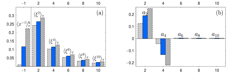
Figure 1: (a) First nonzero moments $\langle{\xi^{N}}\rangle_{\pi}$ (up to $N=10$, see text) and $\langle x^{-1}\rangle^{\textbf{R}}_{\pi}=(1/3)\langle x^{-1}\rangle_{\pi}-1$ of $\varphi_{\text{BMS}}$ (dark bars) with the upper and lower error-bars (grey bars), determined with nonlocal QCD sum rules [9]. (b) Histogram of the first nonzero Gegenbauer coefficients $a_{n}$ of the BMS pion DA and the envelopes of the “bunch” like in (a).

where the index $i$ runs over all scalar, vector, and tensor condensates with dim=6 [9, 8]; $M^{2}$ is the Borel parameter, $s_{\pi}^{0}$ the duality interval in the axial channel. This sum rule allows us to determine the first ten moments $\langle\xi^{N}\rangle_{\pi}\equiv\int_{0}^{1}\varphi_{\pi}(x)(2x-1)^{N}dx$ of the pion DA and independently the inverse moment $\langle x^{-1}\rangle_{\pi}\equiv\int_{0}^{1}\varphi_{\pi}(x)x^{-1}dx$ quite accurately (see in [24] for an illustration). The corresponding Gegenbauer coefficients can be determined (see [9]) from this set within some error range (Fig. 1b) that translates into a “bunch” of pion DAs shown for $\lambda_{q}^{2}=0.4$ GeV² in Fig. 2.

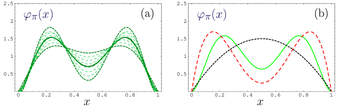
Figure 2: (a) Bunch of pion DAs for $\lambda_{q}^{2}=0.4$ GeV² determined with nonlocal QCD sum rules at normalization scale $\mu\approx 1.0$ GeV. (b) The BMS model [9] (solid line) in comparison with the asymptotic DA (dotted line) and the CZ model (dashed line) [1].

Their striking feature is that their endpoints are suppressed relative to both the CZ model and the asymptotic solution. Crudely speaking, this shape structure is the net result of the interplay between the perturbative contribution and the non-perturbative term $\Delta\Phi_{\text{S}}(x;M^{2})$ (related to the scalar condensate) that dominates the RHS of the SR in Eq. (6). The fact that the function $\Delta\Phi_{\text{S}}(x;M^{2})$ is not singular in $x$ and has a dip at the central point of the interval $[0,1]$ is also reflected in the shapes of these DAs. We emphasize that a suppression of the endpoint region as strong as possible (for a dedicated discussion we refer to [25]) is important in order to improve the self-consistency of perturbative QCD in convoluting the pion DA with the specific hard-scattering amplitude for a particular exclusive process. In order to stress this point, we show in Fig. 3 $\langle x^{-1}\rangle_{\pi}$, calculated as $\int_{x}^{x+0.02}\varphi(x)x^{-1}dx$ and normalized to $100\%$ ($y$-axis).

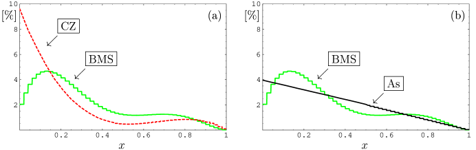
Figure 3: Percentage distribution (see text) of the first inverse moment in $x$ of the BMS model [9] in comparison with rival models.

The main message from this figure is that $\langle x^{-1}\rangle_{\pi}$ receives in the endpoint region, say between $0\leq x\leq 0.1$, a contribution of only 17% in the case of the BMS model, whereas it reaches as much as 40% for the CZ model and still 19% for the asymptotic solution.

3 ANALYSIS OF THE CLEO DATA

It was shown by Khodjamirian [17] that the light-cone QCD sum-rule (LCSR) method provides the possibility to treat the problem of the photon long-distance interaction (i.e., when a photon goes on mass shell) in the $\gamma^{*}(Q^{2})\gamma(q^{2})\to\pi^{0}$ form factor by performing all calculations for sufficiently large $q^{2}$, using quark-hadron duality in the vector channel, and then analytically continuing the results to the limit $q^{2}=0$. Schmedding and Yakovlev (SY) [15] applied these LCSRs to the NLO of QCD perturbation theory. More recently, we have [16] taken up this sort of data processing (i) accounting for a correct Efremov–Radyushkin–Brodsky–Lepage (ERBL) [4, 5] evolution of the pion DA to every measured momentum scale, (ii) estimating more precisely the contribution of the (next) twist-4 term, and (iii) improving the error estimates in determining the $1\sigma$- and $2\sigma$-error contours in the $(a_{2},a_{4})$ plane. Moreover, our error analysis takes into account the variation of the twist-4 contribution and treats the threshold effects in the running of $\alpha_{s}(Q^{2})$ more accurately.

Our procedure is based upon LCSRs for the transition form factor $F^{\gamma^{*}\gamma\pi}(Q^{2},q^{2}\approx 0)$ [17, 15]:

$$F_{\text{LCSR}}^{\gamma^{*}\gamma\pi}(Q^{2})=\frac{1}{\pi}\,\int\limits_{0}^{s_{0}}\!\!\frac{ds}{m_{\rho}^{2}}\,\rho(Q^{2},s;\mu^{2})e^{\left(m_{\rho}^{2}-s\right)/M^{2}}+\frac{1}{\pi}\,\int\limits_{s_{0}}^{\infty}\!\!\frac{ds}{s}\,\rho(Q^{2},s;\mu^{2})\;,$$ (7)

following from a dispersion relation with $M^{2}\approx 0.7$ GeV², where $m_{\rho}$ is the $\rho$-meson mass and $s_{0}=1.5$ GeV² denotes the effective threshold in the $\rho$-meson channel. The spectral density $\rho(Q^{2},s;\mu^{2})\equiv$ $\mathbf{Im}\left[F_{\text{QCD}}^{\gamma^{*}\gamma^{*}\pi}(Q^{2},q^{2}=-s;\mu^{2})\right]$ is calculated by virtue of the factorization theorem for the form factor at Euclidean photon virtualities $q^{2}_{1}=-Q^{2}<0$, $q^{2}_{2}=-q^{2}\leq 0$ [4, 5, 26], and the factorization scale $\mu^{2}$ is fixed by SY at $\mu^{2}=\mu^{2}_{\text{SY}}=5.76~{}\text{GeV}^{2}$. Moreover, $F_{\text{QCD}}^{\gamma^{*}\gamma^{*}\pi}(Q^{2},q^{2};\mu^{2})$ contains a twist-4 contribution, which is proportional to the coupling $\delta^{2}(\mu^{2})$, defined by [17, 27] $\langle\pi(p)|g_{s}\bar{d}\tilde{G}_{\alpha\mu}\gamma^{\alpha}u|0\rangle=i\delta^{2}f_{\pi}p_{\mu}$, where $\tilde{G}_{\alpha\mu}=(1/2)\varepsilon_{\alpha\mu\rho\sigma}G^{\rho\sigma}$ and $G_{\rho\sigma}=G_{\rho\sigma}^{a}\lambda^{a}/2$.

This contribution for the asymptotic twist-4 DAs of the pion as well as explicit expressions for the spectral density $\rho(Q^{2},s;\mu^{2})$ in LO have been obtained in [17] to which we refer for details. The spectral density of the twist-2 part in NLO has been calculated in [15]—see Eqs. (18) and (19) there. All needed expressions for the evaluation of Eq. (7) are collected in the Appendix E of [16], cf. Eqs. (E.1)–(E.3). We set $\mu^{2}=Q^{2}$ in $F_{\text{QCD}}^{\gamma^{*}\gamma^{*}\pi}(Q^{2},q^{2};\mu^{2})$ and use the complete 2-loop expression for the form factor, absorbing the logarithms into the coupling constant and the pion DA evolution at the NLO level [16] so that $\alpha_{s}(\mu^{2})\stackrel{{\scriptstyle\text{RG}}}{{\longrightarrow}}\alpha_{s}(Q^{2})$ and $\varphi_{\pi}(x;\mu^{2})\stackrel{{\scriptstyle\text{ERBL}}}{{\longrightarrow}}\varphi_{\pi}(x;Q^{2})=U(\mu^{2}\to Q^{2})\varphi_{\pi}(x;\mu^{2})$ (RG denotes the renormalization group). Then, we use the spectral density $\rho(Q^{2},s,Q^{2})$, derived in [15] at $\mu^{2}=\mu^{2}_{\text{SY}}$, in Eq. (7) to obtain $F^{\gamma^{*}\gamma\pi}(Q^{2})$ and fit the CLEO data over the probed momentum range, denoted by $\{Q^{2}_{\text{exp}}\}$. In our recent analysis [16] the evolution $\varphi_{\pi}(x;Q^{2})=U(\mu^{2}_{\text{SY}}\to Q^{2})\varphi_{\pi}(x;\mu^{2}_{\text{SY}})$ was performed for every individual point $Q^{2}_{\text{exp}}$, with the aim to return to the normalization scale $\mu^{2}_{\text{SY}}$ and to extract the DA parameters $(a_{2},~{}a_{4})$ at this reference scale for the sake of comparison with the previous SY results [15]. In effect, for every measurement, $\{Q_{\text{exp}}^{2},F^{\gamma^{*}\gamma\pi}(Q_{\text{exp}}^{2})\}$, its own factorization and renormalization scheme was used so that the NLO radiative corrections were taken into account in a complete way.

The accuracy of this procedure is still limited because of the uncertainties entailed by the twist-4 scale parameter [16], $k\cdot\delta^{2}$, with the factor $k$ expressing the deviation of the twist-4 DAs from their asymptotic shapes (another source of uncertainty originates from the unknown NNLO $\alpha_{s}$-corrections, see [16]). Based on our experience with the twist-2 case, we set $k=1\pm 0.1$. As a result, the final (rather conservative) accuracy estimate for the twist-4 scale parameter can be expressed in terms of $k\cdot\delta^{2}(1)=0.19\pm 0.04~{}\text{GeV}^{2}$ [16]. To produce the complete $2\sigma$- and $1\sigma$-contours, corresponding to these uncertainties, we need to unite a number of regions, resulting from the processing of the CLEO data at different values of the scale parameter $k\cdot\delta^{2}$ within this admissible range [16]. The obtained results for the asymptotic DA (◆), the BMS model (✖) [9], the CZ DA (◼), the SY best-fit point (⚫) [15], a recent transverse lattice result (▼) (fourth reference in [13]), and two instanton-based models, viz., (★) [10] and (✦) (using in this latter case $m_{q}=325$ MeV, $n=2$, and $\Lambda=1$ GeV) [11], are displayed in Fig. 4(a) varying the twist-4 scale parameter $k\cdot\delta^{2}$ in the interval $[0.15\leq k\cdot\delta^{2}\leq 0.23]~{}\text{GeV}^{2}$.

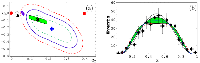
Figure 4: (a) Analysis of the CLEO data on $F_{\pi\gamma^{*}\gamma}(Q^{2})$ in terms of error regions around the best-fit point (✚) (broken line: $1\sigma$; solid line: $2\sigma$; dashed-dotted line: $3\sigma$) in the ($a_{2}$,$a_{4}$) plane contrasted with various theoretical models explained in the text. The slanted shaded rectangle represents the constraints on ($a_{2},~{}a_{4}$) plane posed by the nonlocal QCD sum rules [9] for the value $\lambda^{2}_{q}=0.4$ GeV². All constraints are evaluated at $\mu^{2}_{\text{SY}}=5.76~{}\text{GeV}^{2}$ after NLO ERBL evolution. (b) Comparison of $\varphi^{\text{asy}}$ (solid line), $\varphi^{\text{CZ}}$ (dashed line), and the BMS “bunch” of pion DAs (strip, [16]) with the E791 data [18]. The corresponding $\chi^{2}$ values are: 12.56—asy; 14.15—CZ; 10.96—BMS.

The important points to observe from this figure are these: (i) the nonlocal QCD sum-rule constraints, encoded in the slanted shaded rectangle, are in rather good overall agreement with the CLEO data at the $1\sigma$-level; (ii) the CZ model and the asymptotic DA are ruled out at least at the $3\sigma$-level. These findings are not significantly changed, even if one allows an extreme twist-4 uncertainty of 30%, or if excluding the low-momentum-transfer data tail—say, up to $Q^{2}_{\text{exp}}=3$ GeV² [16]. In the first case, the asymptotic DA is outside the 3$\sigma$-error ellipse, whereas in the second case it remains outside the 2$\sigma$ region with the instanton-inspired models just at the 2$\sigma$-ellipse boundary and the CZ model always far outside.

4 E791 DATA: CONSTRAINTS FROM DIFFRACTIVE DI-JETS PRODUCTION

An independent source of experimental data to constraint the shape of the pion DA is provided by the E791 Fermilab experiment [18]. Unfortunately, these data are affected by inherent uncertainties and their theoretical explanation by different groups [19, 20, 21] is still controversial so that they cannot be used to exclude some optional model. For our exposition here the important point is to show that our predictions for this process are not conflicting the E791 data using for all considered models the same calculational framework, notably the convolution approach of [21]. The results of the calculation are displayed in Fig. 4(b) making evident that the E791 data are relatively in good agreement with our prediction—especially, in the middle $x$ region, where our DAs “bunch” has the largest uncertainties (see Fig. 2a). Note, however, that all theoretical predictions shown in this figure are not corrected for the detector acceptance. For a more precise comparison, this distortion must be taken into account.

5 CONCLUSION

Both analyzed experimental data sets (CLEO [14] and Fermilab E791 [18]) converge to the conclusion that the pion DA is not everywhere a convex function, like the asymptotic one, but has instead two maxima with the end points ($x=0,1$) strongly suppressed—in contrast to the CZ DA. These two key dynamical features of the DA are both controlled by the QCD vacuum inverse correlation length $\lambda_{q}$, whose value suggested by the CLEO data analysis is $\lambda_{q}^{2}\sim 0.4$ GeV² in good compliance with the QCD sum-rule estimates and lattice computations.

References

- [1] V.L. Chernyak and A.R. Zhitnitsky, Phys. Rep. 112 (1984) 173.
- [2] N.G. Stefanis, Eur. Phys. J. directC 1, 7 (1999).
- [3] S.V. Mikhailov and A.V. Radyushkin, JETP Lett. 43 (1986) 712; Sov. J. Nucl. Phys. 49 (1989) 494; Phys. Rev. D 45 (1992) 1754; A.P. Bakulev and A.V. Radyushkin, Phys. Lett. B 271 (1991) 223; A.P. Bakulev and S.V. Mikhailov, Z. Phys. C 68 (1995) 451.
- [4] A.V. Efremov and A.V. Radyushkin, Phys. Lett. B 94 (1980) 245; Theor. Math. Phys. 42 (1980) 97.
- [5] G.P. Lepage and S.J. Brodsky, Phys. Lett. B 87 (1979) 359; Phys. Rev. D 22 (1980) 2157.
- [6] V.M. Braun and I.E. Filyanov, Z. Phys. C 44 (1989) 157.
- [7] V.M. Belyaev and M.B. Johnson, Phys. Rev. D 56 (1997) 1481; Phys. Lett. B 423 (1998) 379.
- [8] A.P. Bakulev and S.V. Mikhailov, Phys. Lett. B 436 (1998) 351.
- [9] A.P. Bakulev, S.V. Mikhailov, and N.G. Stefanis, Phys. Lett. B 508 (2001) 279.
- [10] V.Y. Petrov et al., Phys. Rev. D 59 (1999) 114018.
- [11] M. Praszalowicz and A. Rostworowski, Phys. Rev. D 64 (2001) 074003; ibid. 66 (2002) 054002.
- [12] I.V. Anikin, A.E. Dorokhov, L. Tomio, Phys. Lett. B 475 (2000) 361.
- [13] G. Martinelli and C.T. Sachrajda, Phys. Lett. B 190 (1987) 151; D. Daniel et al., Phys. Rev. D 43 (1991) 3715; M. Burkardt and H. El-Khozondar, Phys. Rev. D 60 (1999) 054504; M. Burkardt and S. Seal, Phys. Rev. D 65 (2002) 034501; S. Dalley and B. van de Sande, Phys. Rev. D 67 (2003) 114507; L. Del Debbio et al., Nucl. Phys. Proc. Suppl. 83 (2000) 235; 119 (2003) 416.
- [14] J. Gronberg et al., CLEO Collaboration, Phys. Rev. D 57 (1998) 33.
- [15] A. Schmedding and O. Yakovlev, Phys. Rev. D 62 (2000) 116002.
- [16] A.P. Bakulev, S.V. Mikhailov, and N.G. Stefanis, Phys. Rev. D 67 (2003) 074012; hep-ph/0303039.
- [17] A. Khodjamirian, Eur. Phys. J. C 6 (1999) 477.
- [18] E.M. Aitala et al., Fermilab E791 Collaboration, Phys. Rev. Lett. 86 (2001) 4768.
- [19] V. Chernyak, Phys. Lett. B 516 (2001) 116.
- [20] N.N. Nikolaev, W. Schäfer, and G. Schwiete, Phys. Rev. D 63 (2001) 014020.
- [21] V.M. Braun et al., Nucl. Phys. B 638 (2002) 111.
- [22] M.A. Shifman, A.I. Vainshtein, and V.I. Zakharov, Nucl. Phys. B 147 (1979) 385, 448, 519.
- [23] A.P. Bakulev and S.V. Mikhailov, Phys. Rev. D 65 (2002) 114511.
- [24] A.P. Bakulev, S.V. Mikhailov, and N.G. Stefanis, in “Proceedings of the 36th Rencontres De Moriond On QCD And Hadronic Interactions, 17–24 Mar 2001, Les Arcs, France”, Ed. J. Tran Thanh Van, Singapour, World Scientific, 2002, pp. 133–136 [hep-ph/0104290].
- [25] N.G. Stefanis et al., Phys. Lett. B 449 (1999) 299; Eur. Phys. J. C 18 (2000) 137.
- [26] F. del Aguila and M.K. Chase, Nucl. Phys. B 193 (1981) 517; E.P. Kadantseva, S.V. Mikhailov, and A.V. Radyushkin, Sov. J. Nucl. Phys. 44 (1986) 326.
- [27] V.A. Novikov et al., Nucl. Phys. B 237 (1984) 525.