SLAC-PUB-10205 hep-ph/0310229 October 2003
Beyond the standard model with $B$ and $K$ physics

Abstract

In the first part of the talk the flavor physics input to models beyond the Standard Model is described. One specific example of such a new physics model is given: a model with bulk fermions in one non-factorizable extra dimension. In the second part of the talk we discuss several observables that are sensitive to new physics. We explain what type of new physics can produce deviations from the Standard Model predictions in each of these observables.

1 Introduction

The success of the Standard Model (SM) can be seen as a proof that it is an effective low energy description of Nature. Yet, there are many reasons to believe that the SM has to be extended. A partial list includes the hierarchy problem, the strong CP problem, baryogenesis, gauge coupling unification, the flavor puzzle, neutrino masses, and gravity. We are therefore interested in probing the more fundamental theory. One way to go is to search for new particles that can be produced in yet unreached energies. Another way to look for new physics is to search for indirect effects of heavy unknown particles. In this talk we explain how flavor physics is used to probe such indirect signals of physics beyond the SM.

2 New Physics and Flavor

In general, flavor bounds provide strong constraints on new physics models. This fact is called “the new physics flavor problem”. The problem is actually the mismatch between the new physics scale that is required in order to solve the hierarchy problem and the one that is needed in order to satisfy the experimental bounds from flavor physics.[1] Here we explain what is the new physics flavor problem, discuss ways to solve it and give one example of a model with interesting, viable, flavor structure.

2.1 The New Physics Flavor Problem

In order to understand what is the new physics flavor problem let us first recall the hierarchy problem.[2] In order to prevent the Higgs mass from getting a large radiative correction, new physics must appear at a scale that is a loop factor above the weak scale

$$\Lambda\mathrel{\hbox to0.0pt{\lower 4.0pt\hbox{\hskip 1.0pt$\sim$}\hss}\raise 1.0pt\hbox{$<$}}4\pi m_{W}\sim 1\;{\rm TeV}.$$ (1)

Here, and in what follows, $\Lambda$ represents the new physics scale. Note that such TeV new physics can be directly probed in collider searches.

While the SM scalar sector is unnatural, its flavor sector is impressively successful. This success is linked to the fact that the SM flavor structure is special. First, the charged current interactions are universal. (In the mass basis, this is manifest through the unitarity of the CKM matrix.) Second, Flavor-Changing-Neutral-Currents (FCNCs) are highly suppressed: they are absent at the tree level and at the one loop level they are further suppressed by the GIM mechanism. These special features are important in order to explain the observed pattern of weak decays. Thus, any extension of the SM must conserve these successful features.

Consider a generic new physics model, that is, a model where the only suppression of FCNCs processes is due to the large masses of the particles that mediate them. Naturally, these masses are of the order of the new physics scale, $\Lambda$. Flavor physics, in particular measurements of meson mixing and CP-violation, put severe constraints on $\Lambda$.

In order to find these bounds we take an effective field theory approach. At the weak scale we write all the non-renormalizable operators that are consistent with the gauge symmetry of the SM. In particular, flavor-changing four Fermi operators of the form (the Dirac structure is suppressed)

$${q_{1}\bar{q}_{2}q_{3}\bar{q}_{4}\over\Lambda^{2}},$$ (2)

are allowed. Here $q_{i}$ can be any quark flavor as long as the electric charges of the four fields in Eq. (2) sum up to zero. The strongest bounds are obtained from meson mixing and CP-violation measurements:

• $K$ physics: $K-\overline{K}$ mixing and CP-violation in $K$ decays imply

  $${s\overline{d}s\overline{d}\over\Lambda^{2}}\quad\mbox{$\Rightarrow$}\quad\Lambda\mathrel{\hbox to0.0pt{\lower 4.0pt\hbox{\hskip 1.0pt$\sim$}\hss}\raise 1.0pt\hbox{$>$}}10^{4}{\mbox{~{}TeV}}.$$ (3)

• $D$ physics: $D-\overline{D}$ mixing implies

  $${c\overline{u}c\overline{u}\over\Lambda^{2}}\quad\mbox{$\Rightarrow$}\quad\Lambda\mathrel{\hbox to0.0pt{\lower 4.0pt\hbox{\hskip 1.0pt$\sim$}\hss}\raise 1.0pt\hbox{$>$}}10^{3}{\mbox{~{}TeV}}.$$ (4)

• $B$ physics: $B-\overline{B}$ mixing and CP-violation in $B$ decays imply

  $${b\overline{d}b\overline{d}\over\Lambda^{2}}\quad\mbox{$\Rightarrow$}\quad\Lambda\mathrel{\hbox to0.0pt{\lower 4.0pt\hbox{\hskip 1.0pt$\sim$}\hss}\raise 1.0pt\hbox{$>$}}10^{3}{\mbox{~{}TeV}}.$$ (5)

Note that the bound from kaon data is the strongest.

There is tension between the new physics scale that is required in order to solve the hierarchy problem, Eq. (1), and the one that is needed in order not to contradict the flavor bounds, Eqs. (3)–(5). The hierarchy problem can be solved with new physics at a scale $\Lambda\sim 1$ TeV. Flavor bounds, on the other hand, require $\Lambda>10^{4}$ TeV. This tension implies that any TeV scale new physics cannot have a generic flavor structure. This is the new physics flavor problem.

Flavor physics has been mainly an input to model building, not an output. The flavor predictions of any new physics model are not a consequence of its generic structure but rather of the special structure that is imposed to satisfy the severe existing flavor bounds.

2.2 Dealing with Flavor

Any viable TeV new physics model has to solve the new physics flavor problem. We now describe several ways to do so that have been used in various models.

$(i)$ Minimal Flavor Violation (MFV) models.[3] In such models the new physics is flavor blind. That is, the only source of flavor violation are the Yukawa couplings. This is not to say that flavor violation arises only from $W$-exchange diagrams via the CKM matrix elements. Other flavor contributions exist, but they are related to the Yukawa interactions. Examples of such models are gauge mediated Supersymmetry breaking models[4] and models with universal extra dimensions.[5] In general, MFV models predict small effects in flavor physics.

$(ii)$ Models with flavor suppression mainly in the first two generations. The hierarchy problem is connected mainly to the third generation since its couplings to the Higgs field are the largest. Flavor bounds, however, are most severe in processes that involve only the first two generations. Therefore, one way to ameliorate the new physics flavor problem is to keep the effective scale of the new physics in the third generation low, while having the effective new physics of the first two generations at a higher scale. Examples of such models include Supersymmetric models with the first two generations of quarks heavy[6] and Randall-Sundrum models with bulk quarks.[7, 8] In general, such models predict large effects in the $B$ and $B_{s}$ systems, and smaller effects in $K$ and $D$ mixings and decays.

$(iii)$ Flavor suppression mainly in the up sector. Since the flavor bounds are stronger in the down sector, one way to go in order to avoid them is to have new flavor physics mainly in the up sector. Examples of such models are Supersymmetric models with alignment[9] and models with discrete symmetries.[10] In general such models predict large effects in charm physics and small effects in $B$, $B_{s}$ and $K$ mixings and decays.

$(iv)$ Generic flavor suppression. In many models some mechanism that suppresses flavor violation for all the quarks is implemented. Examples of such models are Supersymmetric models with spontaneously broken flavor symmetry[11] and models of split fermions in flat extra dimension.[12] In general, such models can be tested with flavor physics.

2.3 An Example: Bulk Quarks in the Randall-Sundrum Model

As discussed above, there are various models that solve the new physics flavor problem in different ways. Here we give one concrete example: the Randall-Sundrum model with bulk quarks[7, 8] which belongs to the class of models that treat the third generation differently than the first two. Thus in this model relatively large effects are expected in the $B$ and $B_{s}$ systems.

The Randall-Sundrum (RS) model solves the hierarchy problem using extra dimensions with non-factorizable geometry. Non-factorizable geometry means that the four-dimensional metric depends on the coordinates of the extra dimensions.[13] In the simplest scenario one considers a single extra dimension, taken to be a $S^{1}/Z_{2}$ orbifold parameterized by a coordinate $y=r_{c}\,\phi$, with $r_{c}$ the radius of the compact dimension, $-\pi\leq\phi\leq\pi$, and the points $(x,\phi)$ and $(x,-\phi)$ identified. There are two 3-branes located at the orbifold fixed points: a “visible” brane at $\phi=\pi$ containing the SM Higgs field, and a “hidden” brane at $\phi=0$. The solution of Einstein’s equations for this geometry leads to the non-factorizable metric

$$\mbox{d}s^{2}=e^{-2kr_{c}|\phi|}\,\eta_{\mu\nu}\,\mbox{d}x^{\mu}\mbox{d}x^{\nu}-r_{c}^{2}\,\mbox{d}\phi^{2}\,,$$ (6)

where $x^{\mu}$ are the coordinates on the four-dimensional surfaces of constant $\phi$, and the parameter $k$ is of order the fundamental Planck scale $M$. (This solution can only be trusted if $k<M$, so the bulk curvature is small compared with the fundamental Planck scale.) The two 3-branes carry vacuum energies tuned such that $V_{\rm vis}=-V_{\rm hid}=-24M^{3}k$, which is required to obtain a solution respecting four-dimensional Poincaré invariance. In between the two branes is a slice of AdS₅ space.

With this setup any mass parameter $m_{0}$ in the fundamental theory is promoted into an effective mass parameter which depends on the location in the extra dimension, $m=e^{-ky}\,m_{0}$. For $y=r_{c}\pi$ and with $kr_{c}\approx 12$ this mechanism produces weak scale physical masses at the visible brane from fundamental masses and couplings of order of the Planck scale.

The SM flavor puzzle can be solved by incorporating bulk fermions in the RS model.[14] Then there are several sources for new contributions to FCNC processes. One of these new sources are non-renormalizable operators which appear with scale of order

$$\Lambda\sim M\exp(-ky^{f}),$$ (7)

where $y^{f}$ is the “localization” point of the fermion $f$. In order to reproduce the observed quark masses and mixing angles,[7, 8] heavy fermions need to have larger $y^{f}$, as can be seen in Fig. 1. Thus, small effects are expected in kaon mixing and decays and large flavor violation effects are expected in $b$ physics.

Figure 1: An example of the shape of the fermion field wave functions in the RS model.[8] $q_{i}^{(0)}$ are the zero mode wave function of the $i$th generation quark doublet ($i=1,2,3$ where $i=1$ is the lightest generation). It can be seen that the third generation doublet is localized toward the visible brane while the first two generation doublets are localized toward the hidden brane. This is the reason that the effective scale of the new physics is smaller for the third generation.

3 Probing New Physics with Flavor

Figure 2: The unitarity triangle.

Any TeV new physics model has to deal with the flavor bounds. Depending on the mechanism that is used to deal with flavor, the prediction of where deviation from the SM can be expected varies. It is important, however, that in many cases large effects are expected. Thus, we hope that we will be able to find such signals.

Generally, it is easier to search for new physics effects where they are relatively large. Namely, in processes that are suppressed in the SM, in particular in:

• meson mixing,

• loop mediated decays, and

• CKM suppressed amplitudes.

It is indeed a major part in the $B$ factories’ program to study such processes. Below we give several examples for ways to search for new physics.

Before proceeding we emphasize the following point: at present there is no significant deviation from the SM predictions in the flavor sector. In the following we give examples of deviations from the SM predictions that are below the $3\sigma$ level. In particular, we choose the following possible tests of the SM:

• global fit,

• $\displaystyle{a_{\rm CP}(B\to\psi K_{S})}$ vs $\displaystyle{a_{\rm CP}(B\to\phi K_{S})}$,

• $B\to K\pi$ decays,

• polarization in $B\to VV$ decays, and

• $K\to\pi\nu\bar{\nu}$ vs $B$ and $B_{s}$ mixing.

There are many more possible tests. Our choice of examples here is partially biased toward cases where the present experimental ranges deviate by more than one standard deviation from the SM predictions. While, as emphasized above, one should not consider these as significant indications for new physics, it should be interesting to follow future improvements in these measurements. Furthermore, it is an instructive exercise to think what one would learn if the central value of these measurements turn out to be correct. As we will see, this would not only indicate new physics, but actually probe the nature of the new physics.

3.1 Global Fit

One way to test the SM is to make many measurements that determine the sides and angles of the unitarity triangle (see Fig. 2), namely, to over-constrain it.[15] Another way to put it is that one tries to measure $\rho$ and $\eta$ in many possible ways. ($\lambda$, $A$, $\rho$ and $\eta$ are the Wolfenstein parameters.) We emphasize that this is not the only way to look for new physics. It is just one among many possible ways to look for new physics.

The global fit is done using measurements of (or bounds on) $|V_{cb}|$, $|V_{ub}/V_{cb}|$, $\varepsilon_{K}$, $B-\overline{B}$ mixing, $B_{s}$ mixing, and $a_{\rm CP}(B\to\psi K_{S})$. The fit is very good, as can be seen in Fig. 3. Clearly, there is no indication for new physics from the global fit. There are many more measurements that at present have very little impact on the fit. In the future, such measurements can be included, and then discrepancies may show up.

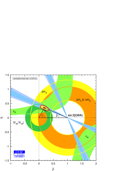
Figure 3: Global fit to the unitarity triangle.[15] The fit is based on the measurements of $|V_{cb}|$, $|V_{ub}/V_{cb}|$, $\varepsilon_{K}$, $B-\overline{B}$ mixing, and $a_{\rm CP}(B\to\psi K_{S})$ and the bound on $B_{s}$ mixing.

3.2 CP-Asymmetries in $b\to s\bar{s}s$ Modes

The time dependent CP-asymmetry in $B$ decays into a CP eigenstate, $f_{CP}$, is given by[16]

$$a_{\rm CP}(B\to f_{CP})\equiv$$

$$~{}~{}{\Gamma(\overline{B}(t)\to f_{CP})-\Gamma(B(t)\to f_{CP})\over\Gamma(\overline{B}(t)\to f_{CP})+\Gamma(B(t)\to f_{CP})}=$$

$$~{}~{}-{(1-|\lambda|^{2})\cos(\Delta m_{B}\,t)-2{\cal I}m\lambda\sin(\Delta m_{B}\,t)\over 1+|\lambda|^{2}}\equiv$$

$$~{}~{}S\,\sin(\Delta m_{B}\,t)-C\,\cos(\Delta m_{B}\,t).$$ (8)

Here $\Delta m_{B}\equiv m_{H}-m_{L}$ and the last line defines $S$ and $C$. Furthermore,

$$\lambda\equiv\left({q\over p}\right)\left({\bar{A}\over A}\right),$$ (9)

where $\bar{A}\equiv A(\overline{B}\to f_{CP})$ and $A\equiv A(B\to f_{CP})$. The neutral $B$ meson mass eigenstates are defined in terms of flavor eigenstates as

$$|B_{L,H}\rangle=p|B\rangle\pm q|\overline{B}\rangle\,.$$ (10)

In the $|\lambda|=1$ limit, which is a very good approximation in many cases, Eq. (3.2) reduces to the simple form

$$a_{\rm CP}(B\to f_{CP})={\cal I}m\lambda\,\sin(\Delta m_{B}\,t)\,.$$ (11)

In that case ${\cal I}m\lambda$ is just the sine of the phase between the mixing amplitude and twice the decay amplitude.

In the SM the mixing amplitude is

$$\arg(A_{mix})=2\beta.$$ (12)

The phase of the decay amplitude depends on the decay mode. $B\to\psi K_{S}$ is mediated by the tree level quark decay $b\to c\bar{c}s$ which has a real amplitude, namely,

$$\arg(A_{b\to c\bar{c}s})=0,$$ (13)

and therefore ${\cal I}m\lambda=\sin 2\beta$. The penguin $b\to s\bar{s}s$ decay amplitude is also real to a good approximation, namely,

$$\arg(A_{b\to s\bar{s}s})=0.$$ (14)

We learn that also in that case ${\cal I}m\lambda=\sin 2\beta$. In particular, the $B\to\phi K_{S}$, $B\to\eta^{\prime}K_{S}$, and $B\to K^{+}K^{-}K_{S}$ are examples of decays that are dominated by the $b\to s\bar{s}s$ transition. They are of particular interest since their CP-asymmetries have been measured. We conclude that to first approximation the SM predicts

$$S_{\psi K_{S}}=-S_{K^{+}K^{-}K_{S}}=S_{\phi K_{S}}=S_{\eta^{\prime}K_{S}}.$$ (15)

The theoretical uncertainties in the above predictions are less than $O(1\%)$ for $S_{\psi K_{S}}$, and of $O(5\%)$ for $S_{\phi K_{S}}$ and $S_{\eta^{\prime}K_{S}}$ and $O(20\%)$ for $S_{K^{+}K^{-}K_{S}}$.[17] Furthermore, for all these modes the SM predicts $|S|=\sin 2\beta$. Note that in order to violate the predictions of Eq. (15), new physics has to affect the decay amplitudes. New physics in the mixing amplitude shifts all the modes by the same amount, leaving Eq. (15) unaffected.

The data do not show a clear picture yet. Using the most recent results,[18] the world averages of the asymmetries are

$$S_{\psi K_{S}} = +0.73\pm 0.05,$$

$$S_{\eta^{\prime}K_{S}} = +0.27\pm 0.21,$$

$$S_{\phi K_{S}} = -0.15\pm 0.70,$$

$$-S_{K^{+}K^{-}K_{S}} = +0.51\pm 0.26^{+0.18}_{-0.00}.$$ (16)

In particular, both $S_{\phi K_{S}}$ and $S_{\eta^{\prime}K_{S}}$ are more then one standard deviation away from $S_{\psi K_{S}}$. (Since the theoretical errors on $S_{K^{+}K^{-}K_{S}}$ are large and due to the brief nature of this talk, we do not discuss this mode any further.)

Figure 4: The $B\to K\pi$ amplitudes. The dominant one is the strong penguin amplitude ($P$), and the sub-dominant ones are the tree amplitude ($T$) and the electroweak penguin amplitude ($P_{EW}$).

Assuming that these anomalies are confirmed in the future, we ask what can explain them. We have to look for new physics that can generate $S_{\psi K_{S}}\neq S_{\phi K_{S}}\neq S_{\eta^{\prime}K_{S}}$. Since $B\to\eta^{\prime}K_{S}$ and $B\to\phi K_{S}$ are one loop processes in the SM, we expect new physics to generate large effects in the CP-asymmetries measured in these modes. Moreover, we expect the shift from $\sin 2\beta$ to be different in the two modes since the ratio of the SM and new physics hadronic matrix elements is in general different. On the contrary, $B\to\psi K_{S}$ is a CKM favored tree level decay in the SM and thus we do not expect new physics to have significant effects. We conclude that new physics in the $b\to s\bar{s}s$ decay amplitude generally gives $S_{\psi K_{S}}\neq S_{\phi K_{S}}\neq S_{\eta^{\prime}K_{S}}$.[20]

It is interesting to ask what we would learn if it turns out that $S_{\psi K_{S}}\neq S_{\phi K_{S}}$ but $S_{\eta^{\prime}K_{S}}$ is consistent with $S_{\psi K_{S}}$. Such a situation can be the result of new parity conserving penguin diagrams.[21, 22] To understand this point note that $B\to\phi K_{S}$ is parity conserving while $B\to\eta^{\prime}K_{S}$ is parity violating. Thus, parity conserving new physics in $b\to s$ penguins only affects $B\to\phi K_{S}$. While generically new physics models are not parity conserving, there are models that are approximately parity conserving. Supersymmetric $SU(2)_{L}\times SU(R)\times{\rm Parity}$ models provide an example of such an approximate parity conserving new physics framework.[21, 22]

3.3 $B\to K\pi$

Consider the four $B\to K\pi$ decays and the underlying quark transitions that mediate them:

$$B^{+}\to K^{0}\pi^{+} \qquad b\to d\bar{d}s,$$

$$B^{+}\to K^{+}\pi^{0} \qquad b\to d\bar{d}s\quad{\rm or}\quad b\to u\bar{u}s,$$

$$B^{0}\to K^{+}\pi^{-} \qquad b\to u\bar{u}s,$$ (17)

$$B^{0}\to K^{0}\pi^{0} \qquad b\to d\bar{d}s\quad{\rm or}\quad b\to u\bar{u}s.$$

In the SM these modes can be used to measure $\gamma$. Moreover, there are many SM relations between these modes that can be used to look for new physics.[23]

There are three main types of diagrams that contribute to these decays. The strong penguin diagram ($P$), the tree diagram ($T$) and the EW penguin diagram ($P_{EW}$); see Fig. 4. It is important to understand the relative magnitudes of these amplitudes. Due to the ratio between the strong and electroweak coupling constants, $P\gg P_{EW}$. The relation between $P$ and $T$ is not as simple. On the one hand, $P$ is a loop amplitude while $T$ is a tree amplitude. On the other hand, the CKM factors in $T$ are $O(\lambda^{2})\sim 0.05$ smaller than in $P$. Thus, it is not clear which amplitude is dominant. Experimentally, it turns out that $P\gg T$. Thus, to first approximation all the four decay rates in Eq. $(\ref{fourbkpi})$ are mediated by the strong penguin amplitude and therefore have the same rate (up to Clebsch-Gordon coefficients). Yet, there are corrections to this expectation due to the sub-leading $T$ and $P_{EW}$ amplitudes.

Due to the hierarchy of amplitudes, there are many approximate relations between the four $B\to K\pi$ decay modes. Let us consider one particular relation, called the Lipkin sum rule.[24] As we explain below the Lipkin sum rule is interesting since the correction to the pure $P$ limit is only second order in the small amplitudes.

The crucial ingredient that is used in order to get useful relations is isospin. Penguin diagrams are pure $\Delta I=0$ amplitudes, while $T$ and $P_{EW}$ have both $\Delta I=0$ and $\Delta I=1$ parts. The Lipkin sum rule, which is based only on isospin, reads[24]

$$R_{L} \equiv {2\Gamma(B^{+}\to K^{+}\pi^{0})+2\Gamma(B^{0}\to K^{0}\pi^{0})\over\Gamma(B^{+}\to K^{0}\pi^{+})+\Gamma(B^{0}\to K^{+}\pi^{-})}$$ (18)

$$= 1+O\left(P_{EW}+T\over P\right)^{2}.$$

Experimentally the ratio was found to be[25]

$$R_{L}=1.24\pm 0.10.$$ (19)

Using theoretical estimates[26] that

$${P_{EW}\over P}\sim{T\over P}\sim 0.1,$$ (20)

we expect

$$R_{L}=1+O(10^{-2}).$$ (21)

We learn that the observed deviation of $R_{L}$ from 1 is an $O(2\sigma)$ effect.

What can explain $R_{L}-1\gg 10^{-2}$? First, note that any new $\Delta I=0$ amplitude cannot significantly modify the Lipkin sum rule since it modifies only $P$. From the measurement of the four $B\to K\pi$ decay rates we roughly know the value of $P$. This tells us that new physics cannot modify $P$ in a significant way. What is needed in order to explain $R_{L}-1\gg 10^{-2}$ are new “Trojan penguins”, $P_{NP}$, which are isospin breaking ($\Delta I=1$) amplitudes. They modify the Lipkin sum rule as follows

$$R_{\rm L}=1+O\left(P_{NP}\over P\right)^{2}.$$ (22)

In order to reproduce the observed central value a large effect is needed, $P_{NP}\approx P/2$.[27] In many models there are strong bounds on $P_{NP}$ from $b\to s\ell^{+}\ell^{-}$. Leptophobic $Z^{\prime}$ is an example of a viable model that can accommodate significant Trojan penguins amplitude.[28]

3.4 Polarization in $B\to VV$ Decays

Consider $B$ decays into light vectors, in particular,

$$B\to\rho\rho,\qquad B\to\phi K^{*},\qquad B\to\rho K^{*}\,.$$ (23)

Due to the left-handed nature of the weak interaction, in the $m_{B}\to\infty$ limit we expect[22, 29]

$${R_{T}\over R_{0}}=O\left({1\over m^{2}_{B}}\right),\qquad{R_{\perp}\over R_{\parallel}}=1+O\left({1\over m_{B}}\right)$$ (24)

where $R_{0}$ ($R_{T}$, $R_{\perp}$, $R_{\parallel}$) is the longitudinal (transverse, perpendicular, parallel) polarization fraction. Recall that $R_{T}=R_{\perp}+R_{\parallel}$ and $R_{0}+R_{T}=1$.

To understand the above power counting consider for simplicity the pure penguin $B\to\phi K^{*}$ decays. It is convenient to work in the helicity basis (${\cal A}_{-}$, ${\cal A}_{+}$ and ${\cal A}_{0}$), which is related to the transversity basis via

$${\cal A}_{\parallel,\perp}={{\cal A}_{+}\pm{\cal A}_{-}\over\sqrt{2}},$$ (25)

and the longitudinal amplitude is the same in the two bases. We consider the factorizable helicity amplitudes, namely, those contributions which can be written in terms of products of decay constants and form factors. In the SM they are proportional to

$$\!\!\!\!{\cal A}_{0}\propto\frac{f_{\phi}m_{B}^{3}}{m_{K^{*}}}\!\left[\left(1+\frac{m_{K^{*}}}{m_{B}}\right)\!A_{1}\!-\!\left(1-\frac{m_{K^{*}}}{m_{B}}\right)\!A_{2}\right]$$ (26)

$$\!\!\!\!{\cal A}_{\pm}\propto f_{\phi}m_{\phi}m_{B}\left[\left(1+\frac{m_{K^{*}}}{m_{B}}\right)\!A_{1}\!\pm\!\left(1-\frac{m_{K^{*}}}{m_{B}}\right)\!V\right],$$

where terms of order $1/m_{B}^{2}$ were neglected. The $A_{1,2}$ and $V$ are the $B\to K^{*}$ form factors, which are all equal in the $m_{B}\to\infty$ limit. [30] Thus, to leading-order in $\alpha_{s}$[31]

$${A_{2}\over A_{1}}\sim{V\over A_{1}}=1+{\cal O}\left(\frac{1}{m_{B}}\right).$$ (27)

Using Eqs. (26) and (27) we see that the helicity amplitudes exhibit the following hierarchy[22, 29]

$${{\cal A}_{+}\over{\cal A}_{0}}\sim{\cal O}\left({1\over m_{B}}\right),\qquad{{\cal A}_{-}\over{\cal A}_{0}}\sim{\cal O}\left({1\over m_{B}^{2}}\right).$$ (28)

Using Eq. (25) the relations in Eq. (24) immediately follow.

An intuitive understanding of these relations can be obtained by considering the helicities of the $q\bar{q}$ pair that make the vector meson. In the valence quark approximation, when they are both right-handed (left-handed) the vector meson has positive (negative) helicity. When they have opposite helicities the vector meson is longitudinally polarized. In the $m_{B}\to\infty$ limit the light quarks are ultra relativistic and their helicities are determined by the chiralities of the weak decay operators. Since the weak interaction involves only left-handed $b$ decays, the three outgoing light fermions do not have the same helicities. For example, the leading operator generates decays of the form

$$\bar{b}\to\bar{s}_{R}s_{L}\bar{s}_{R}.$$ (29)

(The spectator quark does not have preferred helicity.) Since the $\phi$ is made from an $s$ quark and an $\bar{s}$ antiquark, in this limit it has longitudinal helicity. For finite $m_{B}$ each helicity flip reduces the amplitude by a factor of $1/m_{B}$. To get positive helicities one spin flip, that of the $s$ quark, is required. To get negative helicities, spin flips of the two antiquarks are needed.

The relations in Eq. (24) receive factorizable as well as non-factorizable corrections. Some of these corrections have been calculated, with the result that they do not significantly modify the leading-order results.[29] Still, in order to get a clearer picture, more accurate determinations of the corrections are needed.

Observation of $R_{\perp}\gg R_{\parallel}$ would signal the presence of right-handed chirality effective operators in $B$ decays.[21, 22] The hierarchy between ${\cal A}_{+}$ and ${\cal A}_{-}$ generated by the opposite chirality operator, $\tilde{Q}_{i}$, (obtained from $Q_{i}$ via a parity transformation) is flipped compared to the hierarchy generated by the SM operator. Such right-handed chirality operators lead to an enhancement of $R_{T}$ and therefore can also upset the first relation in Eq. (24).

The polarization data are as follows.[25] The longitudinal fraction has been measured in several modes

$${R_{0}(B^{0}\to\phi K^{*0})} {=} {0.58\pm 0.10},$$

$${R_{0}(B^{+}\to\phi K^{*+})} {=} {0.46\pm 0.12},$$

$$R_{0}(B^{+}\to\rho^{0}K^{*+}) = 0.96\pm 0.16,$$

$$R_{0}(B^{+}\to\rho^{+}\rho^{0}) = 0.96\pm 0.07,$$

$$R_{0}(B^{0}\to\rho^{+}\rho^{-}) = 0.99\pm 0.08.$$ (30)

There is only one measurement of the perpendicular polarization[32]

$${R_{\perp}(B^{0}\to\phi K^{*0})}={0.41\pm 0.11}.$$ (31)

Using $R_{0}+R_{\perp}+R_{\parallel}=1$ we extract

$$R_{\parallel}(B^{0}\to\phi K^{*0})=0.01\pm 0.15.$$ (32)

We see that in $B\to\rho\rho$ and $B\to K^{*}\rho$ the SM prediction $R_{T}/R_{0}\ll 1$ is confirmed, although $R_{T}/R_{0}\gg 1/m_{B}^{2}$ remains a possibility. Since in these modes $R_{T}$ is very small, the second SM prediction, $R_{\perp}\approx R_{\parallel}$, cannot be tested yet.

The situation is different in $B\to\phi K^{*}$. First, the data favor ${R_{T}/R_{0}}=O\left(1\right)$, which is not a small number. Second, one also finds that ${R_{\perp}/R_{\parallel}}\gg 1$. Both of these results are in disagreement with the SM predictions in Eq. (24).

It is interesting that the preliminary data indicate that the SM predictions do not hold in $B\to\phi K^{*}$. This is a pure penguin $b\to s\bar{s}s$ decay. The decays where the SM predictions appear to hold, $B\to K^{*}\rho$ and particularly $B\to\rho\rho$, on the other hand, have significant tree contributions. It is thus important to obtain polarization measurements in other modes, especially the pure penguin $b\to s\bar{d}d$ decay $B^{+}\to K^{*0}\rho^{+}$.

With more precise polarization data it may therefore be possible to determine whether or not there are new right-handed currents, and if so whether or not they are only present in $b\to s\bar{s}s$ decays.

3.5 $K\to\pi\nu\bar{\nu}$

The $K\to\pi\nu\bar{\nu}$ decays are very good probes of the unitarity triangle.[33] They are dominated by the $s\to d$ electroweak penguin amplitude with internal top quark which is proportional to $|V_{td}|$. Isospin and perturbative QCD can be used to eliminate almost all the hadronic uncertainties. One more point that makes these modes attractive is that in many cases new physics affects $B$ decays and $K$ decays differently.[34] Then, the apparent determination of the unitarity triangle from these different sources will be different.

Experimentally, there is only a measurement of the decay rate of the charged mode[35]

$${\cal B}(K^{+}\to\pi^{+}\nu\bar{\nu})=(15.7^{+17.5}_{-8.2})\times 10^{-11}.$$ (33)

The SM prediction is[33]

$${\cal B}^{\rm SM}(K^{+}\to\pi^{+}\nu\bar{\nu})=4.4\times 10^{-11}\times\left[\eta^{2}+(1.4-\rho)^{2}\right].$$ (34)

Using the preferred values for $\rho$ and $\eta$ (see Fig. 2), $\rho\sim 0.15$ and $\eta\sim 0.4$, the central value for the SM prediction is[36]

$${\cal B}^{\rm SM}(K^{+}\to\pi^{+}\nu\bar{\nu})\approx 7.7\times 10^{-11}.$$ (35)

We learn that the measurement [Eq. (33)] is in agreement with the SM prediction [Eq. (35)].

It is interesting to ask what one will learn if it turns out that the SM prediction is not confirmed by the data. Let us assume that in the future the measurement of ${\cal B}(K^{+}\to\pi^{+}\nu\bar{\nu})$ will converge around its current central value. Inspecting Eq. (34) we learn that in order to get ${\cal B}(K^{+}\to\pi^{+}\nu\bar{\nu})=15.7\times 10^{-11}$ we need large $\eta$ ($\eta\sim 2$) or negative $\rho$. These possibilities are in conflict with the current global fit of the unitarity triangle; see Fig. 5. Large $\eta$ is in conflict with the measurement of $|V_{ub}|$. Since $|V_{ub}|$ is extracted from tree level processes, its determination is unlikely to be affected by new physics. On the contrary, $\rho<0$ is in conflict with the measurement of $B-\bar{B}$ mixing and the bound on $B_{s}-\bar{B}_{s}$ mixing. These are loop processes, and can be modified in the presence of new physics. We conclude that new physics in $K^{+}\to\pi^{+}\nu\bar{\nu}$ or $B-\bar{B}$ mixing or $B_{s}-\bar{B}_{s}$ mixing can generate such a disagreement.

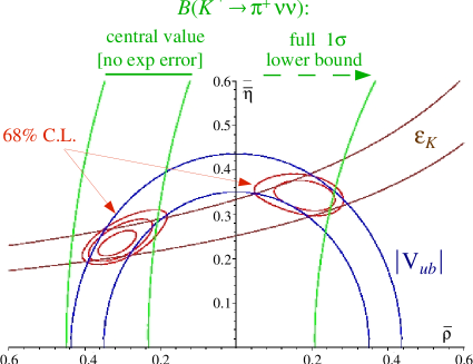
Figure 5: Global fit to the unitarity triangle with the measurement of ${\cal B}(K^{+}\to\pi^{+}\nu\bar{\nu})$.[36] It can be seen that the central value of the measurement is inconsistent with the unitarity triangle extracted from the measurement of $B-\bar{B}$ mixing and the bound on $B_{s}-\bar{B}_{s}$ mixing.

Higher precision in the measurement of ${\cal B}(K^{+}\to\pi^{+}\nu\bar{\nu})$ and a measurement of ${\cal B}(K_{L}\to\pi^{0}\nu\bar{\nu})$ are important in order to further explore this avenue for searching for new physics.

4 Conclusions

The main goal of high energy physics is to find the theory that extends the SM into shorter distances. Flavor physics is a very good tool for such a mission. Depending on the mechanism for suppressing flavor-changing processes, different patterns of deviation from the SM are expected to be found. In some cases almost no deviations are expected, while in other we expect deviations in specific classes of processes. While there is no signal for such new physics yet, there are intriguing results. More data is needed in order to look further for fundamental physics using low energy flavor-changing processes.

References

- [1] For a discussion for Supersymmetric models see, for example, Z. Ligeti and Y. Nir, Nucl. Phys. Proc. Suppl. 111, 82 (2002) [hep-ph/0202117]; Y. Grossman, Y. Nir and R. Rattazzi, Adv. Ser. Direct. High Energy Phys. 15, 755 (1998) [hep-ph/9701231].
- [2] See, for example, M. Schmaltz, Nucl. Phys. Proc. Suppl. 117, 40 (2003) [hep-ph/0210415]; G. F. Giudice, these proceedings.
- [3] For a review see, for example, A. J. Buras, hep-ph/0307203.
- [4] For a review see, Y. Shadmi and Y. Shirman, Rev. Mod. Phys. 72, 25 (2000) [hep-th/9907225].
- [5] Flavor aspects of universal extra dimensions are discussed in A. J. Buras, M. Spranger and A. Weiler, Nucl. Phys. B 660, 225 (2003) [hep-ph/0212143].
- [6] M. Dine, R. G. Leigh and A. Kagan, Phys. Rev. D 48, 4269 (1993) [hep-ph/9304299]; A. Pomarol and D. Tommasini, Nucl. Phys. B 466, 3 (1996) [hep-ph/9507462]; G. R. Dvali and A. Pomarol, Phys. Rev. Lett. 77, 3728 (1996) [hep-ph/9607383]; A. G. Cohen, D. B. Kaplan and A. E. Nelson, Phys. Lett. B 388, 588 (1996) [hep-ph/9607394].
- [7] T. Gherghetta and A. Pomarol, Nucl. Phys. B 586, 141 (2000) [hep-ph/0003129]; S. J. Huber and Q. Shafi, Phys. Lett. B 498, 256 (2001) [hep-ph/0010195]; K. Agashe, A. Delgado, M. J. May and R. Sundrum, hep-ph/0308036; G. Burdman, hep-ph/0310144.
- [8] S. J. Huber, Nucl. Phys. B 666, 269 (2003) [hep-ph/0303183].
- [9] Y. Nir and N. Seiberg, Phys. Lett. B 309, 337 (1993) [hep-ph/9304307]; M. Leurer, Y. Nir and N. Seiberg, Nucl. Phys. B 420, 468 (1994) [hep-ph/9310320].
- [10] For one of the early models see S. Pakvasa and H. Sugawara, Phys. Lett. B 73, 61 (1978).
- [11] M. Leurer, Y. Nir and N. Seiberg, Nucl. Phys. B 398, 319 (1993) [hep-ph/9212278].
- [12] N. Arkani-Hamed and M. Schmaltz, Phys. Rev. D 61, 033005 (2000) [hep-ph/9903417]; Y. Grossman and G. Perez, Phys. Rev. D 67, 015011 (2003) [hep-ph/0210053].
- [13] L. Randall and R. Sundrum, Phys. Rev. Lett. 83, 3370 (1999) [hep-ph/9905221].
- [14] Y. Grossman and M. Neubert, Phys. Lett. B 474, 361 (2000) [hep-ph/9912408].
- [15] A. Hocker, H. Lacker, S. Laplace and F. Le Diberder, Eur. Phys. J. C 21, 225 (2001) [hep-ph/0104062]. Recent fits can be found in the CKMfitter home page at ckmfitter.in2p3.fr.
- [16] For a review, notation and formalism, see Y. Nir, Lectures at XXVII SLAC Summer Institute on Particle Physics, hep-ph/9911321; G.C. Branco, L. Lavoura and J.P. Silva, “CP violation,” Oxford, UK: Clarendon (1999); K. Anikeev et al., hep-ph/0201071.
- [17] Y. Grossman, G. Isidori and M. P. Worah, Phys. Rev. D 58, 057504 (1998) [hep-ph/9708305]; D. London and A. Soni, Phys. Lett. B 407, 61 (1997) [hep-ph/9704277]; M. Beneke and M. Neubert, Nucl. Phys. B 651, 225 (2003) [hep-ph/0210085]; Y. Grossman, Z. Ligeti, Y. Nir and H. Quinn, Phys. Rev. D 68, 015004 (2003) [hep-ph/0303171]; M. Gronau and J. L. Rosner, Phys. Lett. B 564, 90 (2003) [hep-ph/0304178].
- [18] T. Browder, these proceedings.
- [19] K. Hagiwara et al., Particle Data Group, Phys. Rev. D 66, 010001 (2002).
- [20] See, for example, Y. Grossman and M. P. Worah, Phys. Lett. B 395, 241 (1997) [hep-ph/9612269]; A. Kagan, in proceedings of the 7th International Symposium on Heavy Flavor Physics, Santa Barbara, CA July 1997, hep-ph/9806266; R. Fleischer and T. Mannel, Phys. Lett. B 511, 240 (2001) [hep-ph/0103121]; G. Hiller, Phys. Rev. D 66, 071502 (2002) [hep-ph/0207356]; A. Datta, Phys. Rev. D 66, 071702 (2002) [hep-ph/0208016]; M. Raidal, Phys. Rev. Lett. 89, 231803 (2002) [hep-ph/0208091]; R. Harnik, D. T. Larson, H. Murayama and A. Pierce, hep-ph/0212180; C. W. Chiang and J. L. Rosner, Phys. Rev. D 68, 014007 (2003) [hep-ph/0302094]; G. L. Kane, P. Ko, H. b. Wang, C. Kolda, J. h. Park and L. T. Wang, Phys. Rev. Lett. 90, 141803 (2003) [hep-ph/0304239]; A. K. Giri and R. Mohanta, Phys. Rev. D 68, 014020 (2003) [hep-ph/0306041]; J. F. Cheng, C. S. Huang and X. h. Wu, hep-ph/0306086; R. Arnowitt, B. Dutta and B. Hu, hep-ph/0307152.
- [21] A. L. Kagan, lecture at SLAC Summer Institute, August 2002, www.slac.stanford.edu/gen/meeting/ ssi/2002/kagan1.html#lecture2.
- [22] A. L. Kagan, talk at first workshop on the discovery potential of an asymmetric factory at luminosity, May 2003, www.slac.stanford.edu/ BFROOT/www/Organization/1036_Study_Group/ 0303Workshop/index.html
- [23] For recent reviews, see: R. Fleischer, Phys. Rept. 370, 537 (2002) [hep-ph/0207108]; J. L. Rosner, hep-ph/0304200; M. Gronau, hep-ph/0306308.
- [24] H. J. Lipkin, hep-ph/9809347; Phys. Lett. B 445, 403 (1999) [hep-ph/9810351]; M. Gronau and J. L. Rosner, Phys. Rev. D 59, 113002 (1999) [hep-ph/9809384].
- [25] J. Fry, these proceedings.
- [26] M. Beneke, G. Buchalla, M. Neubert and C. T. Sachrajda, Nucl. Phys. B 606, 245 (2001) [hep-ph/0104110].
- [27] M. Gronau and J. L. Rosner, hep-ph/0307095; A. J. Buras, R. Fleischer, S. Recksiegel and F. Schwab, hep-ph/0309012.
- [28] Y. Grossman, M. Neubert and A. L. Kagan, JHEP 9910, 029 (1999) [hep-ph/9909297]; K. Leroux and D. London, Phys. Lett. B 526, 97 (2002) [hep-ph/0111246].
- [29] A. L. Kagan, in preparation.
- [30] J. Charles, A. Le Yaouanc, L. Oliver, O. Pene and J. C. Raynal, Phys. Rev. D 60, 014001 (1999) [hep-ph/9812358]; C. W. Bauer, S. Fleming, D. Pirjol and I. W. Stewart, Phys. Rev. D 63, 114020 (2001) [hep-ph/0011336].
- [31] M. Beneke and T. Feldmann, Nucl. Phys. B 592, 3 (2001) [hep-ph/0008255]; G. Burdman and G. Hiller, Phys. Rev. D 63, 113008 (2001) [hep-ph/0011266].
- [32] [Belle Collaboration], hep-ex/0307014.
- [33] G. Buchalla and A. J. Buras, Phys. Rev. D 54, 6782 (1996) [hep-ph/9607447].
- [34] Y. Grossman and Y. Nir, Phys. Lett. B 398, 163 (1997) [hep-ph/9701313]; Y. Nir and M. P. Worah, Phys. Lett. B 423, 319 (1998) [hep-ph/9711215].
- [35] S. Adler et al. [E787 Collaboration], Phys. Rev. Lett. 88, 041803 (2002) [hep-ex/0111091].
- [36] G. D’Ambrosio and G. Isidori, Phys. Lett. B 530, 108 (2002) [hep-ph/0112135]; G. Isidori, eConf C0304052, WG304 (2003) [hep-ph/0307014].