LMU 18/03

TUM-HEP-519/03

hep-ph/0310219

October 2003

More Model-Independent Analysis of $b\to s$ Processes
Gudrun Hiller
Ludwig-Maximilians-Universität München, Sektion Physik, Theresienstraße 37,
D-80333 München, Germany

Frank Krüger
Physik Department, Technische Universität München,
D-85748 Garching, Germany

We study model-independently the implications of non-standard scalar and pseudoscalar interactions for the decays $b\to s\gamma$, $b\to sg$, $b\to s\ell^{+}\ell^{-}$ ($\ell=e,\mu$) and $B_{s}\to\mu^{+}\mu^{-}$. We find sizeable renormalization effects from scalar and pseudoscalar four-quark operators in the radiative decays and at $O(\alpha_{s})$ in hadronic $b$ decays. Constraints on the Wilson coefficients of an extended operator basis are worked out. Further, the ratios $R_{H}={\mathcal{B}}(B\to H\mu^{+}\mu^{-})/{\mathcal{B}}(B\to He^{+}e^{-})$, for $H=K^{(*)},X_{s}$, and their correlations with the $B_{s}\to\mu^{+}\mu^{-}$ decay are investigated. We show that the Standard Model prediction for these ratios defined with the same cut on the dilepton mass for electron and muon modes, $R_{H}=1+O(m^{2}_{\mu}/m^{2}_{b})$, has a much smaller theoretical uncertainty ($\lesssim 1\%$) than the one for the individual branching fractions. The present experimental limit $R_{K}\leqslant 1.2$ puts constraints on scalar and pseudoscalar couplings, which are similar to the ones from current data on ${\mathcal{B}}(B_{s}\to\mu^{+}\mu^{-})$. We find that new physics corrections to $R_{K^{*}}$ and $R_{X_{s}}$ can reach $13\%$ and $10\%$, respectively.

1 Introduction

Flavor-changing neutral currents (FCNCs) are forbidden in the Standard Model (SM) at tree level and arise only at one loop. Hence, they are sensitive to quantum corrections from heavy degrees of freedom at and above the electroweak scale. The rare decays $b\to s\gamma$, $b\to sg$ and $b\to s\ell^{+}\ell^{-}$, where $\ell=e$ or $\mu$, are such promising probes. Measurements of these processes are rapidly improving by the present generation of $B$ experiments and in the not too distant future by the Tevatron and the LHC. The analysis of $b\to s$ transitions can be systematically performed in terms of an effective low-energy theory with the Hamiltonian (see, e.g., Ref. [1])

$${\mathcal{H}}_{\mathrm{eff}}=-\frac{4G_{F}}{\sqrt{2}}V_{tb}V_{ts}^{*}\sum_{i}[C_{i}(\mu){\mathcal{O}}_{i}(\mu)+C_{i}^{\prime}(\mu){\mathcal{O}}_{i}^{\prime}(\mu)].$$ (1.1)

The operators ${\mathcal{O}}_{i}^{(\prime)}$ in Eq. (1.1) include dipole couplings with a photon and a gluon and dilepton operators with vector and axial-vector, as well as with scalar and pseudoscalar Lorentz structures. They are given as

$${\mathcal{O}}_{7}=\frac{e}{g_{s}^{2}}m_{b}(\bar{s}\sigma_{\mu\nu}P_{R}b)F^{\mu\nu},\quad{\mathcal{O}}_{8}=\frac{1}{g_{s}}m_{b}(\bar{s}_{\alpha}\sigma_{\mu\nu}T^{a}_{\alpha\beta}P_{R}b_{\beta})G^{a\mu\nu},$$

$${\mathcal{O}}_{9}=\frac{e^{2}}{g_{s}^{2}}(\bar{s}\gamma_{\mu}P_{L}b)(\bar{\ell}\gamma^{\mu}\ell),\quad{\mathcal{O}}_{10}=\frac{e^{2}}{g_{s}^{2}}(\bar{s}\gamma_{\mu}P_{L}b)(\bar{\ell}\gamma^{\mu}\gamma_{5}\ell),$$

$${\mathcal{O}}_{S}=\frac{e^{2}}{16\pi^{2}}(\bar{s}P_{R}b)(\bar{\ell}\ell),\quad{\mathcal{O}}_{P}=\frac{e^{2}}{16\pi^{2}}(\bar{s}P_{R}b)(\bar{\ell}\gamma_{5}\ell).$$ (1.2)

The operators ${\mathcal{O}}_{1-6}$ can be seen in Ref. [5]. The primed operators in Eq. (1.1) can be obtained from their unprimed counterparts by replacing $P_{L}\leftrightarrow P_{R}$. In the SM as well as in models with minimal flavor violation (MFV) where flavor violation is entirely ruled by the CKM matrix, the Wilson coefficients $C^{\prime}_{i}$ are suppressed by the strange quark Yukawa coupling

$$C^{\prime}_{i}\sim\frac{m_{s}}{m_{b}}C_{i}.$$ (1.3)

Furthermore, the SM contributions to scalar and pseudoscalar operators due to neutral Higgs-boson exchange are tiny even for taus since

$$C^{\mathrm{SM}}_{S,P}\sim\frac{m_{\ell}m_{b}}{m_{W}^{2}}.$$ (1.4)

Thus, in the context of the SM only the operators ${{\mathcal{O}}}_{7-10}$ matter for semileptonic and radiative $b\to s$ transitions.

Our plan is to determine the coefficients $C_{i}^{(\prime)}$ from a fit to the data and thereby testing the SM [6]. At present the number of measured independent observables is not sufficient, so one currently has to simplify the program and deal with a restricted set of operators. In this work we analyze the decays $B\to X_{s}\gamma$, $B\to X_{s}\ell^{+}\ell^{-}$, $B\to K^{(*)}\ell^{+}\ell^{-}$, $B_{s}\to\mu^{+}\mu^{-}$ with the following assumptions:

• The effects of right-handed currents can be neglected, i.e., $C_{i}^{\prime}\simeq 0$.

• The Wilson coefficients of scalar and pseudoscalar operators are proportional to the lepton mass $C_{S,P}\propto m_{\ell}$ such that the coupling to electrons is negligible. This is automatically fulfilled if $C_{S,P}$ are generated by neutral Higgs-boson exchange, but not in general within SUSY models with broken $R$-parity.

• There are no CP-violating phases from physics beyond the SM.

Therefore we take into account the Wilson coefficients $C_{7-10}$ and $C_{S,P}$. Model-independent analyses of the decays $b\to s\gamma$ and $b\to s\ell^{+}\ell^{-}$ in the framework of the SM operator basis with ${\mathcal{O}}_{7-10}$ have been previously performed in Refs. [8, 9, 10]. Distributions with an extended basis including ${\mathcal{O}}_{S,P}$ were analyzed for $B\to X_{s}\ell^{+}\ell^{-}$ in Refs. [7, 11] and for $B\to K^{*}\ell^{+}\ell^{-}$ decays in Refs. [12, 13] to illustrate possible new physics effects. In these works, however, no correlations between the just-mentioned decay modes and $B_{s}\to\ell^{+}\ell^{-}$ decays have been considered. In Ref. [3] the decays $B_{s}\to\mu^{+}\mu^{-}$ and $B\to K^{(*)}\mu^{+}\mu^{-}$ have been studied model-independently. It has been shown that the Wilson coefficients $C_{S,P}$ can be of $O(1)$ while respecting data on the $B_{s}\to\mu^{+}\mu^{-}$ branching fraction, and thus are comparable in size to the vector and axial-vector couplings. For a combined study of $B_{s}\to\mu^{+}\mu^{-}$ and $B\to X_{s}\mu^{+}\mu^{-}$ decays in the minimal supersymmetric standard model (MSSM), see [14].

We perform here a combined analysis of the $B_{s}\to\mu^{+}\mu^{-}$ branching ratio and the observables

$$R_{H}\equiv\frac{\displaystyle\int_{4m_{\mu}^{2}}^{q^{2}_{\mathrm{max}}}dq^{2}\,\frac{d\Gamma(B\to H\mu^{+}\mu^{-})}{dq^{2}}}{\displaystyle\int_{4m_{\mu}^{2}}^{q^{2}_{\mathrm{max}}}dq^{2}\,\frac{d\Gamma(B\to He^{+}e^{-})}{dq^{2}}},\quad H=X_{s},K^{(*)},$$ (1.5)

where $q^{2}_{\mathrm{max}}=(m_{B}-m_{K^{(*)}})^{2}$ for $B\to K^{(*)}\ell^{+}\ell^{-}$ and $q^{2}_{\mathrm{max}}\approx m_{b}^{2}$ for the inclusive decay modes. We also examine the low dilepton invariant mass region of the inclusive decays below the $J/\psi$ mass with $q^{2}_{\mathrm{max}}=6\ {\mathrm{GeV}}^{2}$. Note that we use the lower cut of $4m_{\mu}^{2}$ for both electron and muon modes in order to remove phase space effects in the ratio $R_{H}$. Within the SM, we obtain clean predictions even for the exclusive decays

$$R_{H}^{\mathrm{SM}}=1+O({m_{\mu}^{2}}/{m_{b}^{2}}),$$ (1.6)

which holds also outside the SM if $C_{S,P}\simeq 0$. The normalization to the $e^{+}e^{-}$ mode in Eq. (1.5) was also discussed in Ref. [15] for the inclusive decays.

This paper is organized as follows. In Sec. 2 we summarize the current experimental status and constraints on the decay modes of interest. Section 3 contains a discussion of new physics contributions to scalar and pseudoscalar four-quark operators and their impact on the Wilson coefficients of the SM operator basis. We investigate new physics effects in the decays $b\to s\gamma$ and $b\to sg$. Model-independent constraints on the coefficients of the operators ${{\mathcal{O}}}_{7-10}$ in the presence of ${{\mathcal{O}}}_{S}$ and ${{\mathcal{O}}}_{P}$ are derived in Sec. 4. In Sec. 5 we study correlations between the branching ratios of the decays $B_{s}\to\mu^{+}\mu^{-}$, $B\to X_{s}\ell^{+}\ell^{-}$ and $B\to K^{(*)}\ell^{+}\ell^{-}$. In particular, quantitative predictions are obtained for the ratios $R_{K^{(*)},X_{s}}$. We summarize and conclude in Sec. 6. The anomalous dimensions, decay distributions for $b\to s\ell^{+}\ell^{-}$ processes and auxiliary coefficients are given in Appendices A–D.

2 Experimental status of $b\to s$ transitions

We summarize recent results on the inclusive and exclusive $b\to s\ell^{+}\ell^{-}$ decay modes in Table 1.

Table 1: Branching fractions for various rare $B$ decays [16, 17, 18, 19]. The inclusive measurements as well as the corresponding theoretical predictions have been obtained for $m_{e^{+}e^{-}}>0.2\ {\mathrm{GeV}}$. The SM predictions are taken from Ref. [9] updated with ${\mathcal{B}}(B\to X_{c}\ell\nu_{\ell})=0.108$.

Decay modes	SM	Belle	BaBar
$B\to X_{s}e^{+}e^{-}$	$(4.3\pm 0.7)\times 10^{-6}$	$(5.0\pm 2.3^{+1.3}_{-1.1})\times 10^{-6}$	$(6.6\pm 1.9^{+1.9}_{-1.6})\times 10^{-6}$
$B\to X_{s}\mu^{+}\mu^{-}$	$(4.3\pm 0.7)\times 10^{-6}$	$(7.9\pm 2.1^{+2.1}_{-1.5})\times 10^{-6}$	$(5.7\pm 2.8^{+1.7}_{-1.4})\times 10^{-6}$
$B\to Ke^{+}e^{-}$	$(3.6\pm 1.2)\times 10^{-7}$	$(4.8^{+1.5}_{-1.3}\pm 0.3\pm 0.1)\times 10^{-7}$	$(7.4^{+1.8}_{-1.6}\pm 0.5)\times 10^{-7}$
$B\to K\mu^{+}\mu^{-}$	$(3.6\pm 1.2)\times 10^{-7}$	$(4.8^{+1.2}_{-1.1}\pm 0.3\pm 0.2)\times 10^{-7}$	$(4.5^{+2.3}_{-1.9}\pm 0.4)\times 10^{-7}$
$B\to K^{*}e^{+}e^{-}$	$(16.4\pm 5.1)\times 10^{-7}$	$(14.9^{+5.2}_{-4.6}{}^{+1.2}_{-1.3}\pm 0.2)\times 10^{-7}$	$(9.8^{+5.0}_{-4.2}\pm 1.1)\times 10^{-7}$
$B\to K^{*}\mu^{+}\mu^{-}$	$(12.4\pm 4.0)\times 10^{-7}$	$(11.7^{+3.6}_{-3.1}\pm 0.9\pm 0.5)\times 10^{-7}$	$(12.7^{+7.6}_{-6.1}\pm 1.6)\times 10^{-7}$

These measurements are in agreement with the SM prediction [9] within errors. The experimental constraints we use in our numerical calculations are given below. Note that throughout this work we do not distinguish between $B$ and $\bar{B}$.

(i) The combined results of Belle [19] and BaBar [16] for the inclusive $b\to s\ell^{+}\ell^{-}$ decays yield the $90\%$ confidence level intervals

$$2.8\times 10^{-6}\leqslant{\mathcal{B}}(B\to X_{s}e^{+}e^{-})\leqslant 8.8\times 10^{-6},$$ (2.1)

$$3.5\times 10^{-6}\leqslant{\mathcal{B}}(B\to X_{s}\mu^{+}\mu^{-})\leqslant 10.4\times 10^{-6}.$$ (2.2)

The statistical significance of the Belle (BaBar) measurements of ${\mathcal{B}}(B\to X_{s}e^{+}e^{-})$ and ${\mathcal{B}}(B\to X_{s}\mu^{+}\mu^{-})$ is $3.4\sigma$ ($4.0\sigma)$ and $4.7\sigma$ ($2.2\sigma$), respectively. To be conservative, we also use in our analysis the ${90\%\ \mathrm{C.L.}}$ limits [20]

$${\mathcal{B}}(B\to X_{s}e^{+}e^{-})<10.1\times 10^{-6},$$ (2.3)

$${\mathcal{B}}(B\to X_{s}\mu^{+}\mu^{-})<19.1\times 10^{-6}$$ (2.4)

and compare their implications with those of Eqs. (2.1) and (2.2).

(ii) For the exclusive decay channels [17, 18] we obtain the following ${90\%\ \mathrm{C.L.}}$ ranges

$$3.9\times 10^{-7}\leqslant{\mathcal{B}}(B\to Ke^{+}e^{-})\leqslant 7.7\times 10^{-7},$$ (2.5)

$$3.0\times 10^{-7}\leqslant{\mathcal{B}}(B\to K\mu^{+}\mu^{-})\leqslant 6.5\times 10^{-7},$$ (2.6)

and

$$6.5\times 10^{-7}\leqslant{\mathcal{B}}(B\to K^{*}e^{+}e^{-})\leqslant 17.9\times 10^{-7},$$ (2.7)

$$6.7\times 10^{-7}\leqslant{\mathcal{B}}(B\to K^{*}\mu^{+}\mu^{-})\leqslant 17.0\times 10^{-7}.$$ (2.8)

(iii) Using the experimental results displayed in Table 1 we find for the ratios $R_{H}$

$$R_{X_{s}}=1.20\pm 0.52,\quad R_{K}=0.81\pm 0.24,\quad\left.R_{K^{*}}\right|_{\mathrm{no\ cut}}=0.98\pm 0.38,$$ (2.9)

which translates into the ${90\%\ \mathrm{C.L.}}$ intervals

$$0.34\leqslant R_{X_{s}}\leqslant 2.06,\quad 0.42\leqslant R_{K}\leqslant 1.20,\quad 0.35\leqslant\left.R_{K^{*}}\right|_{\mathrm{no\ cut}}\leqslant 1.60.$$ (2.10)

Here, $\left.R_{K^{*}}\right|_{\mathrm{no\ cut}}$ is defined as $R_{K^{*}}$ with the lower integration boundary in the electron mode taken to be $4m_{e}^{2}$, since experimental data on the $B\to K^{*}e^{+}e^{-}$ branching ratios are published only for the full phase space region. We do not include effects from the small difference between the lower cut $m_{e^{+}e^{-}}=0.2\ {\mathrm{GeV}}$ of the experimental analysis [16, 19] and $2m_{\mu}$ used here. Furthermore, we neglect contributions to $B\to Ke^{+}e^{-}$ from the region below $q^{2}=4m_{\mu}^{2}$, where the rate is tiny due to the absence of the photon pole. The above ratios should be compared with the predictions of the SM

$$R_{X_{s}}^{\mathrm{SM}}=0.987\pm 0.006,\quad R^{\mathrm{SM}}_{K}=1\pm 0.0001,\quad\left.R_{K^{*}}^{\mathrm{SM}}\right|_{\mathrm{no\ cut}}=0.73\pm 0.01,$$ (2.11)

and

$$\left.R_{X_{s}}^{\mathrm{SM}}\right|_{\mathrm{low\ }q^{2}}=0.977\pm 0.009,\quad R^{\mathrm{SM}}_{K^{*}}=0.991\pm 0.002,$$ (2.12)

where “low $q^{2}$” denotes a cut below 6 $\mbox{GeV}^{2}$. The errors on the inclusive and exclusive ratios are due to a variation of the renormalization scale and of the form factors, respectively, see Secs. 4 and 5.

(iv) The current world average of the inclusive $b\to s\gamma$ branching ratio is [21, 22]

$${\mathcal{B}}(B\to X_{s}\gamma)=(3.34\pm 0.38)\times 10^{-4}$$ (2.13)

with a photon energy cut $E_{\gamma}>m_{b}/20$.

(v) For the purely leptonic decays only upper limits exist. The branching ratio of the $B_{s}\to\mu^{+}\mu^{-}$ decay is constrained at ${90\%\ \mathrm{C.L.}}$ as [23]

$${\mathcal{B}}(B_{s}\to\mu^{+}\mu^{-})<2.0\times 10^{-6}.$$ (2.14)

Note that there are preliminary ${90}\%$ confidence level limits of $9.5\times 10^{-7}$ and $16\times 10^{-7}$ from CDF and DØ, respectively [24].

3 New physics contributions to four-quark operators

In this section we address the question whether new physics contributions to four-quark operators can spoil our model-independent analysis. Firstly, the QCD penguins ${\mathcal{O}}_{3-6}$ appear in the SM and many extensions to lowest order only through operator mixing. They enter the matrix element of $b\to s\gamma$ and $b\to s\ell^{+}\ell^{-}$ decays at the loop level. Hence, their impact is subdominant and new physics effects in QCD penguins are negligible for our analysis within current precision. Secondly, and this will be the important effect discussed in the remainder of this section, it is conceivable that the dynamics which generates large couplings to dileptons, i.e., to the operators ${\mathcal{O}}_{S,P}$, induces contributions to 4-Fermi operators with diquarks as well. We introduce the following fermion $f$ dependent operators

$${\mathcal{O}}_{L}^{f}=(\bar{s}P_{R}b)(\bar{f}P_{L}f),\quad{\mathcal{O}}_{R}^{f}=(\bar{s}P_{R}b)(\bar{f}P_{R}f),$$ (3.1)

where for muons we identify the coefficients $C_{L,R}^{\mu}=e^{2}/(16\pi^{2})(C_{S}\mp C_{P})$. We generalize here our assumption (ii) in the sense that the coupling strength is proportional to the fermion mass $m_{f}$, which naturally arises in models with Higgs-boson exchange. In particular, the corresponding Wilson coefficients for $b$ quarks proportional to $m_{b}$ can be potentially large. As will be discussed in the next section, current experimental data on the branching fraction of $B_{s}\to\mu^{+}\mu^{-}$ imply

$$\sqrt{|C_{L}^{b}(m_{W})|^{2}+|C_{R}^{b}(m_{W})|^{2}}\leqslant\frac{e^{2}}{16\pi^{2}}\frac{{m}_{b}(m_{W})}{m_{\mu}}\sqrt{2(|C_{S}(m_{W})|^{2}+|C_{P}(m_{W})|^{2})}\lesssim 0.06.$$ (3.2)

Here, we anticipated our result in Eq. (4.4), i.e., an upper bound on $|C_{S,P}|$ and evolved according to ${\rm d}(C_{S,P}(\mu)/m_{b}(\mu)){\rm d}\mu=0$, with the running $b$-quark mass in the $\overline{\mathrm{MS}}$ scheme given in Eq. (A).

The Wilson coefficients $C_{L,R}^{b}$ are non-zero to lowest order interactions at the electroweak scale $\mu\sim m_{W}$ and can be significantly larger than the ones of the QCD penguins $C_{3-6}(m_{b})\sim O(10^{-2})$. Hence, we have to study the potential impact of the operators ${\mathcal{O}}_{L,R}^{f}$ on our analysis of $b\to s\gamma$ and $b\to s\ell^{+}\ell^{-}$ decays.

3.1 One-loop mixing with pseudoscalar and scalar operators

Scalar and pseudoscalar four-quark operators enter radiative and semileptonic rare $b\to s$ decays at one-loop level as shown in Fig. 1. To estimate their impact, we insert ${\mathcal{O}}_{L}^{b}$ and ${\mathcal{O}}_{R}^{b}$ into the penguin diagrams with an internal $b$ quark and use fully anticommuting $\gamma_{5}$.

Figure 1: Diagrams with an insertion of four-quark operators which contribute to the renormalization and the matrix element of the operator $\widetilde{\mathcal{O}}_{9}$, and with an on-shell photon and no leptons to $\widetilde{\mathcal{O}}_{7}$.

The contributions from the diagram with closed fermion loop vanish by Dirac trace and by gauge invariance or vector current conservation, i.e., after contraction with the lepton current. For simplicity, we work in the “standard” operator basis $\widetilde{\mathcal{O}}_{i}$ given in Appendix A. We obtain non-vanishing contributions from ${\mathcal{O}}_{R}^{b}$ and ${\mathcal{O}}_{L}^{b}$ to $\widetilde{\mathcal{O}}_{7}$ and $\widetilde{\mathcal{O}}_{9}$, respectively. The diagrams with an internal $s$ quark contribute to the helicity-flipped coefficients. They are suppressed by a factor $m_{s}/m_{b}$ and therefore can be neglected. We obtain the following corrections to the Wilson coefficients at the scale $\mu_{b}=m_{b}$

$$\delta\widetilde{C}_{7}(m_{b})=\frac{1}{6}\ln\frac{m_{W}^{2}}{m_{b}^{2}}C_{R}^{b}(m_{W}),$$ (3.3)

$$\delta\widetilde{C}_{9}(m_{b})=\frac{1}{9}\ln\frac{m_{W}^{2}}{m_{b}^{2}}C_{L}^{b}(m_{W}).$$ (3.4)

These infinite renormalization contributions survive in the limit $\alpha_{s}\to 0$, which is similar to what happens in the SM for the mixing of $\widetilde{\mathcal{O}}_{2}$ onto $\widetilde{\mathcal{O}}_{9}$ [27]. With the upper bound in Eq. (3.2) we find that the new physics effect from ${\mathcal{O}}_{L,R}^{b}$ is small, of the order of one percent for $\widetilde{\mathcal{O}}_{9}$, but $\mbox{a\ few}\times{\mathcal{O}}(10\%)$ for $\widetilde{\mathcal{O}}_{7}$. The reason is simply that $\widetilde{C}_{7}^{\mathrm{SM}}(m_{b})$ is more than an order of magnitude smaller than $\tilde{C}_{9}^{\mathrm{SM}}(m_{b})$, which in addition has a smaller anomalous dimension.

Other operators contributing in the SM but subleading in the decays $b\to s\gamma$ and $b\to s\ell^{+}\ell^{-}$ are also subject to similar new physics effects. To be specific, the Wilson coefficients of the chromomagnetic dipole operator and the QCD penguin operators receive corrections from the diagrams in Fig. 1 with diquarks instead of leptons and the intermediate photon replaced by a gluon. We find

$$\delta\widetilde{C}_{8}(m_{b})=-\frac{1}{2}\ln\frac{m_{W}^{2}}{m_{b}^{2}}C_{R}^{b}(m_{W}),$$ (3.5)

$$\delta\widetilde{C}_{3,5}(m_{b})=-\frac{1}{18}\frac{\alpha_{s}}{4\pi}\ln\frac{m_{W}^{2}}{m_{b}^{2}}C_{L}^{b}(m_{W}),$$ (3.6)

$$\delta\widetilde{C}_{4,6}(m_{b})=\frac{1}{6}\frac{\alpha_{s}}{4\pi}\ln\frac{m_{W}^{2}}{m_{b}^{2}}C_{L}^{b}(m_{W}),$$ (3.7)

which are relevant to hadronic $B$ decays. Quantitatively, the renormalization of the gluon dipole operator can be order one. (We study this in more detail below.) The impact on the QCD penguins can be up to several percent. As mentioned earlier, new physics contributions to the operators $\widetilde{\mathcal{O}}_{3-6}$ are subdominant in $b\to s\gamma$ and $b\to s\ell^{+}\ell^{-}$ decays. Since the renormalization of $\widetilde{\mathcal{O}}_{9}$ by scalar and pseudoscalar operators is small, too, we can safely neglect the effects of induced four-quark operators of the type ${\mathcal{O}}_{L}^{b}$ in our analysis of semileptonic and radiative $b\to s$ decays. We remark that scalar and pseudoscalar operators also mix with the electroweak penguin operators $\widetilde{\mathcal{O}}^{e}_{7-10}$ (see Appendix A) at order $\alpha/4\pi$. We have calculated for completeness the corresponding anomalous dimensions, which can be seen in Appendix B.

To get a more accurate estimate of the new physics corrections to the magnetic penguin operators, we resum the leading logarithms in Eqs. (3.3) and (3.5) by means of the renormalization group equations in the $\overline{\mathrm{MS}}$ scheme [1]. Both operators ${\mathcal{O}}_{R}^{b}$ and ${\mathcal{O}}_{L}^{b}$ induce additional operators under renormalization (see Appendix B). The anomalous dimensions of each set are known at next-to-leading order (NLO) [29], with no mixing between the sets. We have calculated the leading-order mixing of ${\mathcal{O}}_{L,R}^{b}$ onto $\widetilde{\mathcal{O}}_{3-9}$. The anomalous dimensions are given in Appendix B together with the respective leading-order self-mixing of both ${\mathcal{O}}_{R}^{b}$ and ${\mathcal{O}}_{L}^{b}$ sets. Numerically, we obtain

$$\delta\widetilde{C}_{7}(m_{b})\simeq 0.71C_{R}^{b}(m_{W}),\quad\delta\widetilde{C}_{8}(m_{b})\simeq-2.95C_{R}^{b}(m_{W}),$$ (3.8)

which implies sizeable contributions to the branching ratios of the radiative decays. We study the phenomenology in Sec. 3.2.

The mixing of scalar and pseudoscalar operators in Eq. (B.1) onto the dipole operators has been studied previously in the context of the two-Higgs-doublet model [31] and in supersymmetry with gluino contributions to $b\to s\gamma$[32]. While our results agree with the ones presented in Ref. [32], they are at variance with those given in Ref. [31]. In particular, we disagree with the conclusion made therein that the scalar and pseudoscalar operators do not mix with $\widetilde{\mathcal{O}}_{9}$.

3.2 Implications for the decays $b\to s\gamma$ and $b\to sg$

We now investigate the phenomenological consequences of the mixing effects presented above for radiative $B$ decays. To illustrate how large these corrections can be, we normalize the Wilson coefficients in the presence of new physics to the ones in the SM, and denote this ratio by $\xi$, such that $\xi^{\mathrm{SM}}=1$. We obtain to next-to-leading order in the SM operator basis and to leading logarithmic approximation in $C_{R}^{b}$

$$\xi_{7}(m_{b})=0.514+0.450\,\xi_{7}(m_{W})+0.035\,\xi_{8}(m_{W})-2.319\,C_{R}^{b}(m_{W}),$$ (3.9)

$$\xi_{8}(m_{b})=0.542+0.458\,\xi_{8}(m_{W})+19.790\,C_{R}^{b}(m_{W}).$$ (3.10)

Given the upper bound in Eq. (3.2) corrections of up to $14\%$ and $119\%$ to $\xi_{7}$ and $\xi_{8}$ can arise. We work out correlations between $\xi_{7}$ and $\xi_{8}$ from ${\mathcal{B}}(B\to X_{s}\gamma)$ given in Eq. (2.13) and ${\mathcal{B}}(B\to X_{s}g)<9\%$ at $90\%$ C.L. [33], using the analytical formulae of Refs. [34, 35, 36]. We obtain the allowed regions at the $\mu_{b}$ scale shown in Fig. 2 for $C_{R}^{b}(m_{W})=0$ (left plot) and $C_{R}^{b}(m_{W})=0.06$ (right plot). The theoretical uncertainty from the prescription of the charm-quark mass has been taken into account by including both solutions obtained for $m_{c}/m_{b}=0.22$ and $0.29$ [37]. From Fig. 2 we see that $A_{7}=0$ for $C_{R}^{b}(m_{W})=0.06$ is allowed by present data on the $b\to sg$ branching fraction. This particular scenario could be excluded by an improved experimental analysis of $b\to sg$. Also, if $C_{R}^{b}(m_{W})$ is near its upper bound, it implies a contribution to the matching conditions for $\widetilde{C}_{7,8}(m_{W})$ in order to be consistent with experimental data.

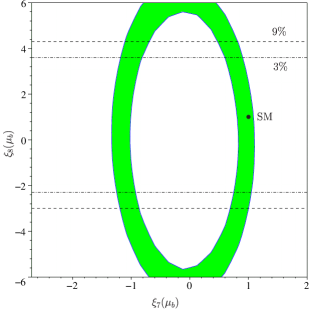
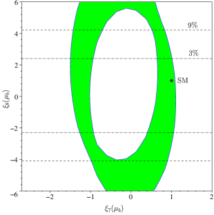
Figure 2: Constraints on $\xi_{7,8}(\mu_{b})$ from ${\mathcal{B}}(b\to s\gamma)$ for $C_{R}^{b}(M_{W})=0$ (left plot) and $C_{R}^{b}(M_{W})=0.06$ (right plot). We also show the upper and lower bounds on $\xi_{8}(\mu_{b})$ for the experimental limit ${\mathcal{B}}(B\to X_{s}g)<9\%$ [33] (dashed lines) and for an assumed value of ${\mathcal{B}}(B\to X_{s}g)<3\%$ (dash-dotted lines).

In summary, we find that the impact of $C_{L}^{b}$ on the matrix element of $\widetilde{\mathcal{O}}_{9}$ is small, at most a few percent, and thus can be neglected. On the other hand, contributions to the dipole operators are in general non-negligible. They can be avoided assuming $C_{R}^{b}(m_{W})\simeq 0$, i.e.,

$$C_{S}+C_{P}=0.$$ (3.11)

In the remainder of this work we discuss the phenomenology with and without this constraint. Note that the absence of logarithms in the matching conditions for $\widetilde{C}_{7,8}(m_{W})$ from neutral Higgs-boson exchange in a two-Higgs-doublet model type II [38, 26] is consistent with the fact that in this model Eq. (3.11) is satisfied [2]. This is also the case for the MSSM with MFV at large $\tan\beta$ [3].

4 Model-independent analysis

In this section we give the theoretical framework that we use to analyze the decays $B\to X_{s}\gamma$, $B\to X_{s}\ell^{+}\ell^{-}$, $B\to K^{(*)}\ell^{+}\ell^{-}$, $B_{s}\to\mu^{+}\mu^{-}$. We then work out model-independent constraints on the coefficients of the operators ${\mathcal{O}}_{7-10}$ and ${\mathcal{O}}_{S,P}$.

4.1 Wilson coefficients and matrix elements

The matrix element of inclusive $b\to s\ell^{+}\ell^{-}$ decays contains contributions from the photon dipole operator ${\mathcal{O}}_{7}$, the dilepton operators ${{\mathcal{O}}}_{9,10}$ and in models beyond the SM also from ${{\mathcal{O}}}_{S,P}$. The decay distributions in the SM are known to next-to-next-to-leading order (NNLO) [5, 39, 40, 41], which corresponds to NLO in $b\to s\gamma$. We use the NNLO expressions for the operators ${\mathcal{O}}_{7,9,10}$ and lowest order ones for ${\mathcal{O}}_{S,P}$ since $O(\alpha_{s})$ corrections to the matrix elements of leptonic scalar and pseudoscalar operators in these decays are not known.

Further, we assume that the contribution from intermediate charmonia has been removed with experimental cuts. Non-perturbative corrections [42] affect the branching ratio by at most few percent and we do not consider them here. We neglect the mass of the strange quark but keep the muon mass consistently, because according to our assumption (ii) also $C_{S,P}$ counts as one power of $m_{l}$ and can be enhanced in models beyond the SM.

The dilepton invariant mass spectra for inclusive and exclusive $b\to s\ell^{+}\ell^{-}$ decays are given in Appendix C. The effective coefficients which enter the decay distributions are written as [5, 39]

$$\widetilde{C}_{7}^{\mathrm{eff}}=\Bigg{[}1+\frac{\alpha_{s}(\mu)}{\pi}\omega_{7}(\hat{s})\Bigg{]}A_{7}(\mu)-\frac{\alpha_{s}(\mu)}{4\pi}\Bigg{[}\sum_{i=1,2}F^{(7)}_{i}(\hat{s})C_{i}^{(0)}(\mu)+F^{(7)}_{8}(\hat{s})A_{8}^{(0)}(\mu)\Bigg{]},$$ (4.1)

$$\widetilde{C}_{9}^{\mathrm{eff}} = \Bigg{[}1+\frac{\alpha_{s}(\mu)}{\pi}\omega_{9}(\hat{s})\Bigg{]}[A_{9}(\mu)+T_{9}h(\hat{m}_{c}^{2},\hat{s})+U_{9}h(1,\hat{s})+W_{9}h(0,\hat{s})]$$ (4.2)

$$- \frac{\alpha_{s}(\mu)}{4\pi}\Bigg{[}\sum_{i=1,2}F^{(9)}_{i}(\hat{s})C_{i}^{(0)}(\mu)+F^{(9)}_{8}(\hat{s})A_{8}^{(0)}(\mu)\Bigg{]},$$

$$\widetilde{C}_{10}^{\mathrm{eff}}=\Bigg{[}1+\frac{\alpha_{s}(\mu)}{\pi}\omega_{9}(\hat{s})\Bigg{]}A_{10}(\mu),$$ (4.3)

where $\hat{m}_{c}=m_{c}/m_{b}$, $\hat{s}=q^{2}/m_{b}^{2}$ and $A_{i},T_{9},U_{9},W_{9}$ are given in Appendix D. The function $h(z,\hat{s})$ originates from the one-loop matrix elements of the four-quark operators ${\mathcal{O}}_{1-6}$ (see Fig. 1) and can be found in Ref. [5]. The functions $\omega_{i},F_{ij}$ arise from real and virtual $\alpha_{s}$ corrections. They can be seen in Refs. [5, 39] together with $\omega_{79}$ which replaces $\omega_{7}$ and $\omega_{9}$ in the interference term ${\mathrm{Re}}\,(\widetilde{C}_{7}^{\mathrm{eff}}\widetilde{C}_{9}^{\mathrm{eff}\ast})$ in the decay rate. In the calculation of the decay rate we expand in powers of $\alpha_{s}$ and retain only linear terms. Note that the $\omega_{i}$ include only that part from real gluon emission which is required to cancel the divergence from the virtual corrections to the matrix element of the ${\mathcal{O}}_{i}$. Further gluon bremsstrahlung corrections in $b\to s\ell^{+}\ell^{-}$ decays [43, 40] are subdominant over the whole phase space except for very low dilepton mass and are not taken into account here. In our numerical analysis we choose a low value for the renormalization scale, $\mu_{b}=2.5\ {\mathrm{GeV}}$, because this approximates the full NNLO dilepton spectrum by the partial one, i.e., with the virtual $O(\alpha_{s})$ corrections $F_{1,2,8}^{(7,9)}=0$ in Eqs. (4.1) and (4.2) switched off [9]. This is beneficial since the $F_{ij}$ are known in a compact analytical form only for the low dilepton invariant mass region [39]. For the exclusive $B\to K^{(*)}\ell^{+}\ell^{-}$ decays we set $\omega_{i}=0$, since these corrections are already included in the corresponding form factors. We do not take into account hard spectator interactions [44].

Below we work out model-independent bounds on $A_{i}\equiv A_{i}^{\mathrm{SM}}+A_{i}^{\mathrm{NP}}$. They differ from the “true” Wilson coefficients $C_{i}$ by penguin contributions that restore the renormalization scheme independence of the matrix element [27]. In addition $A_{9}$ contains logarithms from insertions of the four-quark operators ${\mathcal{O}}_{1-6}$ into the diagrams of Fig. 1. Explicit formulae relating $A_{i}$ and $C_{i}$ are given in Appendix D. As discussed in Sec. 3, we neglect new physics contributions to the QCD penguin operators. In our numerical study we use $f_{B_{s}}=200\ {\mathrm{MeV}}$ and $238\ {\mathrm{MeV}}$ [45] and the parameters given in Table II of Ref. [9] except for ${\mathcal{B}}(B\to X_{c}\ell\nu_{\ell})=10.80\%$ [46]. Form factors and their variation are taken from Ref. [10]. We give the SM values for completeness: $A_{7}^{\mathrm{SM}}(2.5\ {\mathrm{GeV}})=-0.330$, $A_{9}^{\mathrm{SM}}(2.5\ {\mathrm{GeV}})=4.069$ and $A_{10}^{\mathrm{SM}}=-4.213$.

4.2 Constraints from $B_{s}\to\mu^{+}\mu^{-}$

An upper limit on the $B_{s}\to\mu^{+}\mu^{-}$ branching ratio constrains the scalar and pseudoscalar couplings

$$\sqrt{|C_{S}(\mu)|^{2}+|C_{P}(\mu)+\delta_{10}(\mu)|^{2}} \leqslant 3.3\Bigg{[}\frac{{\mathcal{B}}(B_{s}\to\mu^{+}\mu^{-})}{2.0\times 10^{-6}}\Bigg{]}^{1/2}$$ (4.4)

$$\times \Bigg{[}\frac{|V_{tb}V^{*}_{ts}|}{0.04}\Bigg{]}^{2}\Bigg{[}\frac{{m}_{b}(\mu)}{4.4\ {\mathrm{GeV}}}\Bigg{]}\Bigg{[}\frac{238\ {\mathrm{MeV}}}{f_{B_{s}}}\Bigg{]}\Bigg{[}\frac{1/133}{\alpha}\Bigg{]}.$$

Here, we neglected the factor $(1-4{m}_{\mu}^{2}/m_{B_{s}}^{2})$ in front of $|C_{S}|^{2}$, see Eq. (C.3), and defined $\delta_{10}(\mu)=2m_{\mu}{m}_{b}(\mu)/m_{B_{s}}^{2}A_{10}$. The bound given in Eq. (2.14) also implies the upper limits

$${\mathcal{B}}(B_{s}\to e^{+}e^{-})\leqslant 4.7\times 10^{-11},\quad{\mathcal{B}}(B_{s}\to\tau^{+}\tau^{-})\leqslant 4.2\times 10^{-4}.$$ (4.5)

4.3 Constraints from $b\to s\gamma$

The measured $b\to s\gamma$ branching fraction puts constraints on the dipole operators. In the absence of scalar and pseudoscalar couplings $C_{R}^{b}$ (see Sec. 3), which renormalize both electromagnetic and gluonic operators, the two solutions $A_{7}(\mu_{b})\sim\pm A_{7}^{\mathrm{SM}}(\mu_{b})$ are allowed. This is the case if Eq. (3.11) is satisfied. We update the NLO analyses of [9, 35] with the inclusive $b\to s\gamma$ measurement in Eq. (2.13) and ${\mathcal{B}}(B\to X_{c}e\bar{\nu}_{e})=10.80\%$ and obtain the ranges ($\mu_{b}=2.5\ {\mathrm{GeV}}$)

$$-0.36\leqslant A_{7}\leqslant-0.17\quad\mbox{or}\quad 0.21\leqslant A_{7}\leqslant 0.42.$$ (4.6)

The corresponding correlation between $A_{7}$ and $A_{8}$ can be seen in the left plot of Fig. 2. For $C_{R}^{b}(m_{W})=0.06$, on the other hand, the experimental constraints on $A_{7}$ are much weaker (right plot of Fig. 2).

4.4 Constraints from $b\to sl^{+}l^{-}$

In the presence of new physics contributions proportional to the lepton mass we use data on the electron modes to constrain the dilepton couplings $A_{9,10}$. From the upper bound on ${\mathcal{B}}(B\to X_{s}e^{+}e^{-})$ given in Eq. (2.3) we obtain

$$\sqrt{\left|A_{9}\mbox{}^{-0.58}_{+1.05}\right|^{2}+|A_{10}|^{2}} \leqslant \left\{\begin{array}[]{l}9.0\quad\mathrm{for}\quad A_{7}<0\\ 8.9\quad\mathrm{for}\quad A_{7}>0\end{array}\right.$$ (4.9)

$$\sqrt{\left|A_{9}+0.15\right|^{2}+|A_{10}|^{2}} \leqslant \hskip 9.49997pt9.1\quad\mathrm{for}\quad A_{7}=0.$$ (4.10)

The range on ${\mathcal{B}}(B\to X_{s}e^{+}e^{-})$ given in Eq. (2.1) yields upper and lower bounds

$$\left.\begin{array}[]{l}3.8\\ 3.3\end{array}\right\}\leqslant\sqrt{\left|A_{9}\mbox{}^{-0.58}_{+1.05}\right|^{2}+|A_{10}|^{2}}\leqslant\left\{\begin{array}[]{l}8.4\quad\mathrm{for}\quad A_{7}<0\\ 8.3\quad\mathrm{for}\quad A_{7}>0\end{array}\right.$$ (4.15)

$$\hskip 15.07993pt4.8\leqslant\sqrt{\left|A_{9}+0.15\right|^{2}+|A_{10}|^{2}}\leqslant 8.5\quad\mathrm{for}\quad A_{7}=0.$$ (4.16)

Similar bounds can be obtained from data on the muon modes together with the upper limit on $C_{S,P}$ in Eq. (4.4). The lower limit on ${\mathcal{B}}(B\to X_{s}\mu^{+}\mu^{-})$ in Eq. (2.2) yields

$$\sqrt{\left|A_{9}\mbox{}^{-1.4}_{+1.9}\right|^{2}+|A_{10}|^{2}} \geqslant \left\{\begin{array}[]{l}3.8\ (3.5)\quad\mathrm{for}\quad A_{7}<0\\ 3.5\ (3.2)\quad\mathrm{for}\quad A_{7}>0\end{array}\right.$$ (4.19)

$$\sqrt{\left|A_{9}+0.15\right|^{2}+|A_{10}|^{2}} \geqslant \hskip 9.49997pt4.7\ (4.4)\quad\mathrm{for}\quad A_{7}=0$$ (4.20)

for $f_{B_{s}}=238\ {\mathrm{MeV}}$ ($200\ {\mathrm{MeV}})$. Our constraints on $A_{9,10}$ given in Eqs. (4.9)–(4.19) are displayed in Fig. 3. Like in the analysis with the restricted SM basis in [9], $A_{9}=A_{10}=0$ is excluded even in the presence of new scalar and pseudoscalar interactions.

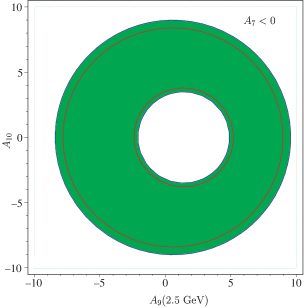
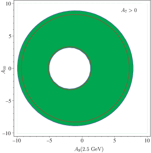
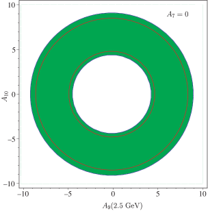
Figure 3: Allowed regions in the $A_{9}$–$A_{10}$ plane in the presence of scalar and pseudoscalar operators from data on inclusive $b\to s\ell^{+}\ell^{-}$ and $b\to s\gamma$ decays for different values of $A_{7}$. The shaded areas are obtained from the upper bound on ${\mathcal{B}}(B\to X_{s}e^{+}e^{-})$ and the lower bound on ${\mathcal{B}}(B\to X_{s}\mu^{+}\mu^{-})$, Eqs. (4.9) and (4.19) with $f_{B_{s}}=200\ {\mathrm{MeV}}$. The two remaining contours indicate the allowed regions from the ${90\%\ \mathrm{C.L.}}$ measurement of ${\mathcal{B}}(B\to X_{s}e^{+}e^{-})$ given in Eq. (4.15). Since the bounds from ${\mathcal{B}}(B\to X_{s}\mu^{+}\mu^{-})$ for $f_{B_{s}}=238\ {\mathrm{MeV}}$ give very similar results, we do not show the corresponding contours.

4.5 Constraints from $R_{K}$

The experimental bound $R_{K}\leqslant 1.2$ in Eq. (2.10) provides constraints on the scalar and pseudoscalar Wilson coefficients complementary to those from the $B_{s}\to\mu^{+}\mu^{-}$ branching fraction given in Eq. (4.4). Varying $A_{7,9,10}$ according to Eqs. (4.6), (4.9)–(4.19) we obtain ($\mu_{b}=2.5\ {\mathrm{GeV}}$)

$$\sqrt{|C_{S}|^{2}+|C_{P}+\Delta_{10}|^{2}}\leqslant 4.5.$$ (4.21)

Here, $\Delta_{10}$ stems from the interference term of $C_{P}$ and $A_{10}$ in the $B\to K\mu^{+}\mu^{-}$ rate, see Eq. (C.4), which can be neglected for large values of $C_{S,P}$. If the bound on $R_{K}$ improves e.g. to 1.1, then the value on the r.h.s. of the above equation changes to 3.2.

5 Correlation between $B_{s}\to\mu^{+}\mu^{-}$ and $b\to s\ell^{+}\ell^{-}$ decays

In this section we study correlations between the ratios $R_{H}$ defined in Eq. (1.5) and ${\mathcal{B}}(B_{s}\to\mu^{+}\mu^{-})$. We restrict ourselves to the case $C_{S}=-C_{P}$, hence a vanishing $A_{7}$ is excluded as shown in Sec. 3.2. We further assume that $A_{9,10}$ are SM valued while $A_{7}$ is allowed to vary in the intervals given in Eq. (4.6). This particular scenario is, for example, realized in the MSSM with MFV at large $\tan\beta$. The maximum values of $R_{H}$ are summarized in Table 2 of Sec. 6 for different new physics scenarios.

The correlations depend sensitively on the decay constant of the $B_{s}$ meson. We display our results for $f_{B_{s}}=200\ {\mathrm{MeV}}$ and $238\ {\mathrm{MeV}}$ except for the inclusive decays, where we vary between these two values. As described in Sec. 4 we use the partial NNLO expressions. Therefore, the plots are obtained for fixed renormalization scale $\mu_{b}=2.5$ GeV. For the analysis of the exclusive decays we show the uncertainty from the form factors.

The SM predictions for the ratios $R_{H}$ are summarized in Eqs. (2.11) and (2.12). The theoretical uncertainty for the inclusive decays is due to the variation of the renormalization scale between $2.5\ {\mathrm{GeV}}$ and $10\ {\mathrm{GeV}}$. Since we are using the partial NNLO expressions this small error below one percent on $R_{X_{s}}^{SM}$ might even be overestimated. For comparison, we give the corresponding numbers at NLO $R_{X_{s}}^{\mathrm{SM},\mathrm{NLO}}=0.974\pm 0.006$ and $R_{X_{s}}^{\mathrm{SM},\mathrm{NLO}}|_{\mathrm{low\ }q^{2}}=0.972\pm 0.005$. The SM prediction for the $B_{s}\to\mu^{+}\mu^{-}$ branching ratio is $(3.6\pm 1.4)\times 10^{-9}$, where the main theoretical uncertainty results from the $B_{s}$ decay constant. It can be considerably reduced once the $B_{s}^{0}$–$\bar{B}^{0}_{s}$ mass difference is known [47].

5.1 Exclusive $B\to K\ell^{+}\ell^{-}$ decays

Figure 4 shows the correlation between $R_{K}$ and the $B_{s}\to\mu^{+}\mu^{-}$ branching ratio for two values of the $B_{s}$-meson decay constant and different signs of $A_{7}$ and $C_{P}$. As illustrated by the solid lines in the upper left plot, the dependence of $R_{K}$ on the form factors is very small and hence this observable is useful for testing the SM. For comparison, the uncertainty on the $B\to K\ell^{+}\ell^{-}$ branching fraction due to the form factors is $\sim 30\%$ [9]. While being consistent with $B_{s}\to\mu^{+}\mu^{-}$ data given in Eq. (2.14), an enhancement of $R_{K}^{\mathrm{SM}}$ by $\sim 60\%$ is excluded by the current upper limit on $R_{K}$ (dotted lines).

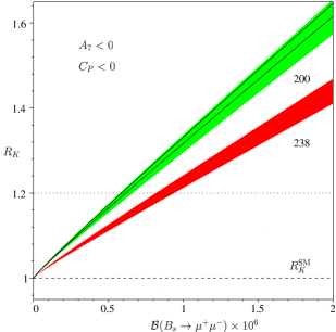
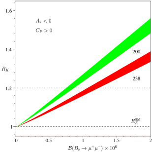
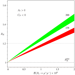
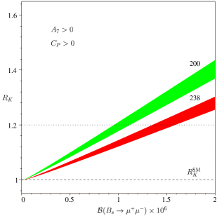
Figure 4: Correlation between $R_{K}$ and the $B_{s}\to\mu^{+}\mu^{-}$ branching ratio for different signs of $A_{7}$ and $C_{P}$, two values of $f_{B_{s}}$ in ${\mathrm{MeV}}$ and $A_{9,10}=A_{9,10}^{\mathrm{SM}}$. The shaded areas have been obtained by varying the $B\to K$ form factors according to Ref. [10] and $A_{7}$ as given in Eq. (4.6). In the upper left plot, the form factor uncertainty is illustrated for fixed $A_{7}=A_{7}^{\mathrm{SM}}$ and $f_{B_{s}}=200\ {\mathrm{MeV}}$ by solid lines. The dotted lines correspond to the ${90\%\ \mathrm{C.L.}}$ upper limit on $R_{K}$ in Eq. (2.10). Dashed lines denote the SM prediction for $R_{K}$.

Furthermore, the ratio $R_{K}$ provides a bound on $C_{S,P}$ which is competitive with the limit from ${\mathcal{B}}(B_{s}\to\mu^{+}\mu^{-})$ in Eq. (4.4). For two values of $R_{K}$ we find ($\mu_{b}=2.5\ {\mathrm{GeV}}$)

$$\sqrt{|C_{S}|^{2}+|C_{P}-0.4|^{2}}\leqslant\left\{\begin{array}[]{l}3.2\quad\mathrm{for}\quad R_{K}=1.2\\ 2.3\quad\mathrm{for}\quad R_{K}=1.1,\end{array}\right.$$ (5.3)

whereas data on $B_{s}\to\mu^{+}\mu^{-}$ decays give

$$\sqrt{|C_{S}|^{2}+|C_{P}-0.15|^{2}}\leqslant 3.8\Bigg{[}\frac{{\mathcal{B}}(B_{s}\to\mu^{+}\mu^{-})}{2.0\times 10^{-6}}\Bigg{]}^{1/2}\Bigg{[}\frac{238\ {\mathrm{MeV}}}{f_{B_{s}}}\Bigg{]}.$$ (5.4)

We recall that $R_{K}=1.2$ corresponds to the current ${90\%\ \mathrm{C.L.}}$ upper limit, see Eq. (2.10).

5.2 Exclusive $B\to K^{*}\ell^{+}\ell^{-}$ decays

The results for $R_{K^{*}}$ versus the branching ratio of $B_{s}\to\mu^{+}\mu^{-}$ are shown in Fig. 5. Note that the variation from the form factors is much larger than in $R_{K}$. This is caused by the form factor $A_{0}$, which drives the $C_{S,P}$ contributions to $R_{K^{*}}$. Its theoretical uncertainty in light cone QCD sum rules [10], which we use in our analysis, is twice as large as in $f_{0}$ relevant for $R_{K}$. New physics effects in $R_{K^{*}}$ can be as large as $30\%$ [allowed by $B_{s}\to\mu^{+}\mu^{-}$ data in Eq. (2.14)] but are restricted to be less than $12\%$ once data on $R_{K}$ are taken into account. For the ratio with no lower cut on the electron mode we find including all constraints $R_{K^{*}}|_{\mathrm{no\ cut}}\leqslant 1.01$, an enhancement of $36\%$ over its SM value.

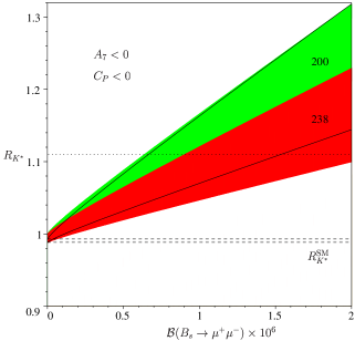
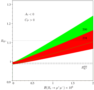
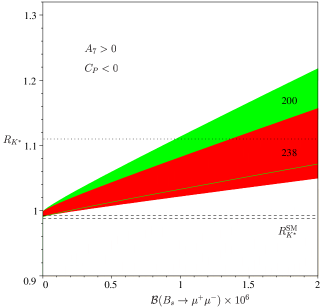
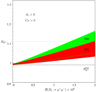
Figure 5: Correlation between $R_{K^{*}}$ and the $B_{s}\to\mu^{+}\mu^{-}$ branching ratio (see Fig. 4 for details). The dotted lines represent the maximum value of $R_{K^{*}}$ consistent with the experimental upper limit $R_{K}\leqslant 1.2$. Dashed lines denote the SM prediction for $R_{K^{*}}$.

5.3 Inclusive $B\to X_{s}\ell^{+}\ell^{-}$ decays

In Fig. 6 we show the correlation of $R_{X_{s}}$ with the $B_{s}\to\mu^{+}\mu^{-}$ branching ratio for the full spectrum with $\hat{s}_{\mathrm{max}}\approx 1$ (upper plots) and for the low dilepton mass with $\hat{s}_{\mathrm{max}}=0.26$ (lower plots). Order one effects in $R_{X_{s}}$ from scalar and pseudoscalar interactions are excluded by current data on $B_{s}\to\mu^{+}\mu^{-}$, contrary to the results of Ref. [15] but in agreement with Ref. [48]. We find a maximum value of $R_{X_{s}}$ of $1.08$ (full spectrum) and $1.05$ (low dilepton mass) from the experimental upper limit on $R_{K}$. These bounds on the $B\to X_{s}\mu^{+}\mu^{-}$ branching ratio are similar to the ones from $B_{s}\to\mu^{+}\mu^{-}$ data previously obtained in [48]. While an enhancement of the $B\to X_{s}\mu^{+}\mu^{-}$ branching ratio of $O(10\%)$ is within the uncertainty of the SM prediction, a corresponding effect in the ratios $R_{X_{s}}$ can be well distinguished from the SM ones.

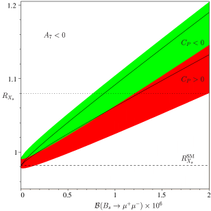
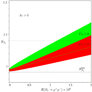
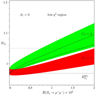
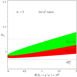
Figure 6: The dependence of $R_{X_{s}}$ on the $B_{s}\to\mu^{+}\mu^{-}$ branching ratio for different signs of $A_{7}$ and $C_{P}$, and $A_{9,10}=A_{9,10}^{\mathrm{SM}}$. The upper plots correspond to the whole dilepton invariant mass spectrum while the lower ones correspond to the low-$q^{2}$ region as described in the text. The shaded areas have been obtained by varying $f_{B_{s}}$ between $200\ {\mathrm{MeV}}$ and $238\ {\mathrm{MeV}}$ and $A_{7}$ according to Eq. (4.6). In the left plots, the solid lines indicate the uncertainty from the variation of $f_{B_{s}}$ for fixed $A_{7}=A_{7}^{\mathrm{SM}}$ and $C_{P}<0$. The dotted lines represent the maximum allowed values of $R_{X_{s}}$ obtained for $R_{K}\leqslant 1.2$. Dashed lines denote the SM prediction for $R_{X_{s}}$.

6 Summary

We performed for the first time a model-independent analysis of $b\to s$ processes in an extended operator basis, the SM one with ${\mathcal{O}}_{7-10}$ plus scalar and pseudoscalar operators ${\mathcal{O}}_{S,P}$ with dileptons. In our phenomenological analysis we took into account experimental constraints from inclusive $b\to s\gamma$, $b\to s\ell^{+}\ell^{-}$ ($\ell=e,\mu$) and $B_{s}\to\mu^{+}\mu^{-}$ decays. Further, we used data on the ratio of $B\to K\mu^{+}\mu^{-}$ to $B\to Ke^{+}e^{-}$ branching ratios, $R_{K}$. We made a few assumptions to facilitate this analysis: no right-handed currents, the couplings to the scalar and pseudoscalar operators are driven by the respective fermion mass and no CP violation beyond the CKM matrix.

We studied the effects of scalar and pseudoscalar operators involving $b$ quarks ${\mathcal{O}}^{b}_{L,R}$. Already at zeroth order in the strong coupling constant these operators mix onto the SM basis: ${\mathcal{O}}^{b}_{L}$ proportional to $C_{S}-C_{P}$ onto the 4-Fermi operators with dileptons and ${\mathcal{O}}^{b}_{R}$ proportional to $C_{S}+C_{P}$ onto the photonic and gluonic dipole operators. Furthermore, we find that the QCD penguins get renormalized at $O(\alpha_{s})$ by ${\mathcal{O}}^{b}_{L}$. While being negligible in $b\to s\ell^{+}\ell^{-}$, these corrections are important for hadronic $b$ decays. In particular, they cancel the strong $\mu$ dependence of the $B\to\phi K_{S}$ amplitude reported recently in Ref. [28]. The lowest order anomalous dimensions involving ${\mathcal{O}}^{b}_{R}$ and the dipole operators have been calculated before in Ref. [32], whereas the ones with ${\mathcal{O}}^{b}_{L}$ and the 4-Fermi operators are a new result of this work. Numerically, we find that for $C_{S}=-C_{P}$ the effects of ${\mathcal{O}}^{b}_{L,R}$ are negligible for our model-independent analysis. However, for $C_{S}\neq-C_{P}$ there is a significant impact from scalar and pseudoscalar couplings on the dipole operators. In particular, the branching ratio for the decay $b\to s\gamma$ can be obtained completely without any contribution from the electromagnetic dipole operator ${\mathcal{O}}_{7}$. This rather extreme scenario could be excluded by improved data on the $b\to sg$ branching ratio, as illustrated in Fig. 2. Except for the case of $A_{7}\simeq 0$, the bounds we obtain on the coefficients $A_{9,10}$ are similar to previous results in the SM operator basis [9]. The non-trivial renormalization effects we encountered show that a model-independent analysis can be quite involved in an enlarged operator basis.

Table 2: Upper bounds on the ratios $R_{H}$ for different $C_{S,P}$ scenarios for $A_{9,10}$ being SM-like and in parentheses without this constraint. Data on $b\to s\gamma$, $b\to s\ell^{+}\ell^{-}$, $B_{s}\to\mu^{+}\mu^{-}$ and $R_{K}$ are taken into account.

Ratio	SM	$C_{S,P}=0$	$C_{S}=-C_{P}$	$C_{S}\neq-C_{P}$
$R_{K}$	1.00	1.00 (1.00)	$1.20$ $(1.20)$	$1.20$ $(1.20)$
$R_{K^{*}}$	$0.99$	1.00 (1.00)	1.11 (1.12)	1.12 (1.12)
$\left.R_{K^{*}}\right|_{\mathrm{no\ cut}}$	$0.74$	0.91 (0.97)	1.01 (1.07)	1.11 (1.12)
$R_{X_{s}}$	$0.98$	0.99 (0.99)	1.08 (1.08)	1.08 (1.08)
$\left.R_{X_{s}}\right|_{\mathrm{low\ }q^{2}}$	$0.97$	0.99 (0.99)	1.05 (1.06)	1.07 (1.07)

We worked out correlations between the ratios $R_{H}$ defined in Eq. (1.5) and the $B_{s}\to\mu^{+}\mu^{-}$ branching ratio for $C_{S}=-C_{P}$ and $A_{9,10}$ being SM-like, summarized in Figs. 4–6. This particular scenario also applies to the MSSM with MFV at large $\tan\beta$. Figure 4 shows that a bound on $R_{K}$ implies a bound on ${\mathcal{B}}(B_{s}\to\mu^{+}\mu^{-})$ and vice versa. Current data on these observables yield very similar constraints on $C_{S,P}$ given in sections 4 and 5. Note that in the above-mentioned MSSM scenario ${\mathcal{B}}(B_{s}\to\mu^{+}\mu^{-})$ and $B^{0}_{s}$–$\bar{B}^{0}_{s}$ mixing are correlated [26]. A similar correlation between $R_{K}$ and in general with larger theoretical errors also with the other $R$’s and $B_{s}^{0}$–$\bar{B}^{0}_{s}$ mixing then holds in this model, too. We stress that in our analysis we take into account information on branching ratios only from inclusive decays. The data on exclusive decays enter our analysis only via $R_{K}$ which depends only weakly on the form factors, as can be seen from Fig. 4. The largest theoretical uncertainty in the correlations is due to the $B_{s}$-meson decay constant.

We further calculated the maximal allowed values of the ratios $R_{H}$, summarized in Table 2. Since we use the partial NNLO expressions for the Wilson coefficients, they have been obtained at the scale $\mu_{b}=2.5$ GeV. We see that large, order one corrections to the respective SM values are already excluded. Note that these upper bounds are insensitive to $f_{B_{s}}$ because current data on $R_{K}\leqslant 1.2$ are here more constraining than ${\mathcal{B}}(B_{s}\to\mu^{+}\mu^{-})$. The effect from $C_{S,P}$ on $B\to K$ decays is always bigger than on $B\to K^{*}$ and $B\to X_{s}$ decays. The reason is that besides different hadronic matrix elements in these decays the photon pole $|A_{7}|^{2}/\hat{s}$, which is absent in the $B\to K$ decay, dominates the rate for very low dilepton mass. The inclusive decay with the spectrum integrated only over the low dilepton invariant mass is even less sensitive, since the lepton-mass-dependent contributions are suppressed by small $\hat{s}$, see Eq. (C.18).

Contributions from scalar and pseudoscalar operators with $V+A$ handedness can be included in the $B_{s}\to\ell^{+}\ell^{-}$ branching ratio by $C_{S,P}\to C_{S,P}-C_{S,P}^{\prime}$ and into the $B\to K\ell^{+}\ell^{-}$ spectrum by $C_{S,P}\to C_{S,P}+C_{S,P}^{\prime}$. Hence, the correlations we presented between ${\mathcal{B}}(B_{s}\to\mu^{+}\mu^{-})$ and $R_{K}$ break down if both chirality contributions $C_{S,P}$ and $C_{S,P}^{\prime}$ are non-vanishing. Since $R_{K}$ constrains the sum and $B_{s}\to\mu^{+}\mu^{-}$ the difference of the coefficients, combining these two [Eqs. (4.4) and (4.21)] yields an upper bound on the magnitude of the individual coefficients of $|C_{S,P}^{(\prime)}|\leqslant 4.3$. This excludes large cancellations and holds even with right-handed contributions to the SM operator basis.

In conclusion, $b\to s\ell^{+}\ell^{-}$ induced decays can have a splitting in the branching ratios depending on the final lepton flavor from physics beyond the SM. Hence, averaging of electron and muon data has to be done carefully in order not to yield a model-dependent result. The effect from scalar and pseudoscalar couplings is best isolated in the theoretically clean observables $R_{H}$ with the same cuts on the dilepton mass. On the other hand, the ratio $R_{K^{*}}|_{\mathrm{no\ cut}}$ constructed with physical phase space boundaries is also sensitive to new physics not residing in $C_{S,P}$, as can be seen from Table 2.

Note added. The lowest order mixing of scalar and pseudoscalar operators onto the SM basis calculated in Sec. 3.1 has been taken into account in a revised version of the first paper of Ref. [28].

Appendix A Standard operator basis

In this appendix we give the “standard” operator basis [1]

$$\widetilde{{{\mathcal{O}}}}_{1}=(\bar{s}_{\alpha}\gamma_{\mu}P_{L}c_{\beta})(\bar{c}_{\beta}\gamma^{\mu}P_{L}b_{\alpha}),\quad\quad\widetilde{{{\mathcal{O}}}}_{2}=(\bar{s}_{\alpha}\gamma_{\mu}P_{L}c_{\alpha})(\bar{c}_{\beta}\gamma^{\mu}P_{L}b_{\beta}),$$

$$\widetilde{{{\mathcal{O}}}}_{3}=(\bar{s}_{\alpha}\gamma_{\mu}P_{L}b_{\alpha})\sum_{q=u,d,s,c,b}(\bar{q}_{\beta}\gamma^{\mu}P_{L}q_{\beta}),\quad\quad\widetilde{{{\mathcal{O}}}}_{4}=(\bar{s}_{\alpha}\gamma_{\mu}P_{L}b_{\beta})\sum_{q=u,d,s,c,b}(\bar{q}_{\beta}\gamma^{\mu}P_{L}q_{\alpha}),$$

$$\widetilde{{{\mathcal{O}}}}_{5}=(\bar{s}_{\alpha}\gamma_{\mu}P_{L}b_{\alpha})\sum_{q=u,d,s,c,b}(\bar{q}_{\beta}\gamma^{\mu}P_{R}q_{\beta}),\quad\quad\widetilde{{{\mathcal{O}}}}_{6}=(\bar{s}_{\alpha}\gamma_{\mu}P_{L}b_{\beta})\sum_{q=u,d,s,c,b}(\bar{q}_{\beta}\gamma^{\mu}P_{R}q_{\alpha}),$$

$$\widetilde{\mathcal{O}}_{7}^{{e}}=\frac{3}{2}(\bar{s}_{\alpha}\gamma_{\mu}P_{L}b_{\alpha})\sum_{q}Q_{q}(\bar{q}_{\beta}\gamma^{\mu}P_{R}q_{\beta}),\quad\widetilde{\mathcal{O}}_{8}^{{e}}=\frac{3}{2}(\bar{s}_{\alpha}\gamma_{\mu}P_{L}b_{\beta})\sum_{q}Q_{q}(\bar{q}_{\beta}\gamma^{\mu}P_{R}q_{\alpha}),$$

$$\widetilde{\mathcal{O}}_{9}^{{e}}=\frac{3}{2}(\bar{s}_{\alpha}\gamma_{\mu}P_{L}b_{\alpha})\sum_{q}Q_{q}(\bar{q}_{\beta}\gamma^{\mu}P_{L}q_{\beta}),\quad\widetilde{\mathcal{O}}_{10}^{{e}}=\frac{3}{2}(\bar{s}_{\alpha}\gamma_{\mu}P_{L}b_{\beta})\sum_{q}Q_{q}(\bar{q}_{\beta}\gamma^{\mu}P_{L}q_{\alpha}),$$

$$\widetilde{\mathcal{O}}_{7}=\frac{e}{16\pi^{2}}m_{b}(\bar{s}_{\alpha}\sigma_{\mu\nu}P_{R}b_{\alpha})F^{\mu\nu},\quad\widetilde{\mathcal{O}}_{8}=\frac{g_{s}}{16\pi^{2}}m_{b}(\bar{s}_{\alpha}\sigma_{\mu\nu}T^{a}_{\alpha\beta}P_{R}b_{\beta})G^{a\mu\nu},$$

$$\widetilde{\mathcal{O}}_{9}=\frac{e^{2}}{16\pi^{2}}(\bar{s}_{\alpha}\gamma_{\mu}P_{L}b_{\alpha})(\bar{\ell}\gamma^{\mu}\ell),\quad\widetilde{\mathcal{O}}_{10}=\frac{e^{2}}{16\pi^{2}}(\bar{s}_{\alpha}\gamma_{\mu}P_{L}b_{\alpha})(\bar{\ell}\gamma^{\mu}\gamma_{5}\ell).$$ (A.1)

Here $Q_{q}$ denotes the charge of the $q$ quark in units of $e$, $\alpha$, $\beta$ are color indices, $a$ labels the SU(3) generators, $P_{L,R}=(1\mp\gamma_{5})/2$ and $m_{b}=m_{b}(\mu)$ is the running mass in the $\overline{\mbox{MS}}$ scheme,

$$m_{b}(\mu)=m^{\rm pole}_{b}\Bigg{[}1-\frac{\alpha_{s}(m^{\rm pole}_{b})}{4\pi}\frac{16}{3}\Bigg{]}\Bigg{[}\frac{\alpha_{s}(\mu)}{\alpha_{s}(m^{\rm pole}_{b})}\Bigg{]}^{\frac{\gamma_{m}^{(0)}}{2\beta_{0}}}\Bigg{\{}1+\Bigg{[}\frac{\gamma_{m}^{(1)}}{2\beta_{0}}-\frac{\beta_{1}\gamma_{m}^{(0)}}{2\beta_{0}^{2}}\Bigg{]}\frac{\alpha_{s}(\mu)-\alpha_{s}(m^{\rm pole}_{b})}{4\pi}\Bigg{\}},$$

with $\gamma^{(0)}_{m}=8$, $\gamma_{m}^{(1)}=1012/9$, $\beta_{0}=23/3$, $\beta_{1}=116/3$.

Appendix B New operators and mixing

The new physics operators containing scalar, pseudoscalar and tensor interactions are written as

$$\widetilde{{{\mathcal{O}}}}_{11}=(\bar{s}_{\alpha}P_{R}b_{\alpha})(\bar{b}_{\alpha}P_{L}b_{\alpha}),\quad\quad\widetilde{{{\mathcal{O}}}}_{12}=(\bar{s}_{\alpha}P_{R}b_{\beta})(\bar{b}_{\beta}P_{L}b_{\alpha}),$$

$$\widetilde{{{\mathcal{O}}}}_{13}=(\bar{s}_{\alpha}P_{R}b_{\alpha})(\bar{b}_{\alpha}P_{R}b_{\alpha}),\quad\quad\widetilde{{{\mathcal{O}}}}_{14}=(\bar{s}_{\alpha}P_{R}b_{\beta})(\bar{b}_{\beta}P_{R}b_{\alpha}),$$

$$\widetilde{{{\mathcal{O}}}}_{15}=(\bar{s}_{\alpha}\sigma_{\mu\nu}P_{R}b_{\alpha})(\bar{b}_{\alpha}\sigma^{\mu\nu}P_{R}b_{\alpha}),\quad\quad\widetilde{{{\mathcal{O}}}}_{16}=(\bar{s}_{\alpha}\sigma_{\mu\nu}P_{R}b_{\beta})(\bar{b}_{\beta}\sigma^{\mu\nu}P_{R}b_{\alpha}),$$ (B.1)

where $\sigma_{\mu\nu}=(i/2)[\gamma_{\mu},\gamma_{\nu}]$ and $\widetilde{{{\mathcal{O}}}}_{11,13}\equiv{{{\mathcal{O}}}}_{L,R}^{b}$ in Eq. (3.1). For completeness, we give their lowest order self mixing [29, 32, 49], i.e., among $\widetilde{{{\mathcal{O}}}}_{11},\widetilde{{{\mathcal{O}}}}_{12}$

$$\gamma=\frac{\alpha_{s}}{4\pi}\left(\begin{array}[]{cc}-16&0\\ -6&2\end{array}\right)$$ (B.4)

and among $\widetilde{{{\mathcal{O}}}}_{13},\dots,\widetilde{{{\mathcal{O}}}}_{16}$

$$\gamma=\frac{\alpha_{s}}{4\pi}\left(\begin{array}[]{cccc}-16&0&{1}/{3}&-1\\ -6&2&-{1}/{2}&-{7}/{6}\\ 16&-48&{16}/{3}&0\\ -24&-56&6&-{38}/{3}\end{array}\right).$$ (B.9)

We obtain the following lowest order anomalous dimensions for the mixing of $\widetilde{{{\mathcal{O}}}}_{13},\dots,\widetilde{{{\mathcal{O}}}}_{16}$ onto $\widetilde{{{\mathcal{O}}}}_{7,8}$

$$\gamma_{13-16,7}=Q_{d}(1,N_{c},-[4+8N_{c}],-[4N_{c}+8]),\quad\gamma_{13-16,8}=(1,0,-4,-8),$$ (B.10)

and of $\widetilde{{{\mathcal{O}}}}_{11,12}$ onto $\widetilde{{{{\mathcal{O}}}}}_{3},\dots,\widetilde{{{{\mathcal{O}}}}}_{6},\widetilde{{{\mathcal{O}}}}_{9}$

$$\gamma_{11,3-6}=\frac{\alpha_{s}}{4\pi}\frac{1}{3}\left(\frac{1}{N_{c}},-1,\frac{1}{N_{c}},-1\right),\quad\gamma_{12,3-6}=0,\quad\gamma_{11,9}=\frac{2Q_{d}}{3},\quad\gamma_{12,9}=N_{c}\frac{2Q_{d}}{3},$$ (B.11)

where $N_{c}$ is the number of colors. Note that Eq. (B.10) is in agreement with [32]. For the mixing of $\widetilde{\mathcal{O}}_{11,12}$ onto the electroweak penguins $\widetilde{\mathcal{O}}_{7}^{{e}},\dots,\widetilde{\mathcal{O}}_{10}^{{e}}$, we find

$$\gamma^{e}_{11,7-10}=-\frac{\alpha}{4\pi}\frac{4Q_{d}}{9}(1,0,1,0),\quad\gamma^{e}_{12,7-10}=-\frac{\alpha}{4\pi}N_{c}\frac{4Q_{d}}{9}(1,0,1,0).$$ (B.12)

The remaining leading order anomalous dimensions vanish.

Appendix C Differential decay distributions

We neglect the $s$-quark mass and introduce the notation

$$\hat{m}_{i} = m_{i}/m_{B},\quad\hat{s}=q^{2}/m_{B}^{2},\quad\hat{u}(\hat{s})=\sqrt{\lambda\left(1-\frac{4\hat{m}_{\ell}^{2}}{\hat{s}}\right)},$$

$$\lambda \equiv 1+\hat{m}_{K^{(*)}}^{4}+\hat{s}^{2}-2\hat{s}-2\hat{m}_{K^{(*)}}^{2}(1+\hat{s})$$ (C.1)

for the exclusive decays and

$$\hat{m}_{i} = m_{i}/m_{b}^{\mathrm{pole}},\quad\hat{s}=q^{2}/(m_{b}^{\mathrm{pole}})^{2}$$ (C.2)

for the inclusive modes. Then, the various decay distributions in the presence of scalar and pseudoscalar operators can be written as follows.

C.1 $B_{s}\to\ell^{+}\ell^{-}$

$$\Gamma(B_{s}\to\ell^{+}\ell^{-}) = \frac{G_{F}^{2}\alpha^{2}m_{B_{s}}^{3}f_{B_{s}}^{2}}{64\pi^{3}}|V_{tb}V_{ts}^{\ast}|^{2}\sqrt{1-\frac{4m_{\ell}^{2}}{m_{B_{s}}^{2}}}$$ (C.3)

$$\times \Bigg{\{}\Bigg{(}1-\frac{4m_{\ell}^{2}}{m_{B_{s}}^{2}}\Bigg{)}\Bigg{|}\frac{m_{B_{s}}C_{S}}{{m}_{b}}\Bigg{|}^{2}+\Bigg{|}\frac{m_{B_{s}}C_{P}}{{m}_{b}}+\frac{2m_{\ell}}{m_{B_{s}}}A_{10}\Bigg{|}^{2}\Bigg{\}},$$

with $A_{10}$ defined in Eq. (D.4) and $C_{S,P}\equiv C_{S,P}(\mu)$, $m_{b}\equiv m_{b}(\mu)$.

C.2 $B\to K\ell^{+}\ell^{-}$

$$\frac{d\Gamma(B\to K\ell^{+}\ell^{-})}{d\hat{s}}=\frac{G_{F}^{2}\alpha^{2}m_{B}^{5}}{2^{10}\pi^{5}}\left|V_{tb}V_{ts}^{\ast}\right|^{2}\hat{u}(\hat{s})\Bigg{\{}(|A^{\prime}|^{2}+|C^{\prime}|^{2})\Bigg{[}\lambda-\frac{\hat{u}(\hat{s})^{2}}{3}\Bigg{]}$$ (C.4)

$$+ 4|C^{\prime}|^{2}\hat{m}_{\ell}^{2}(2+2\hat{m}_{K}^{2}-\hat{s})+8{\mathrm{Re}}\,(C^{\prime}D^{\prime*})\hat{m}_{\ell}^{2}(1-\hat{m}_{K}^{2})+4|D^{\prime}|^{2}\hat{m}_{\ell}^{2}\hat{s}+|T_{P}|^{2}\hat{s}+|T_{S}|^{2}(\hat{s}-4\hat{m}_{\ell}^{2})$$

$$+ 4{\mathrm{Re}}\,(D^{\prime}T^{*}_{P})\hat{m}_{\ell}\hat{s}+4{\mathrm{Re}}\,(C^{\prime}T^{*}_{P})\hat{m}_{\ell}(1-\hat{m}_{K}^{2})\Bigg{\}},$$

with

$$A^{\prime}=\widetilde{C}_{9}^{\mathrm{eff}}(\hat{s})f_{+}(\hat{s})+\frac{2\hat{m}_{b}}{1+\hat{m}_{K}}\widetilde{C}_{7}^{\mathrm{eff}}f_{T}(\hat{s}),$$ (C.5)

$$C^{\prime}=\widetilde{C}^{\mathrm{eff}}_{10}f_{+}(\hat{s}),$$ (C.6)

$$D^{\prime}=\frac{1-\hat{m}_{K}^{2}}{\hat{s}}\widetilde{C}^{\mathrm{eff}}_{10}[f_{0}(\hat{s})-f_{+}(\hat{s})],$$ (C.7)

$$T_{S,P}=\frac{1-\hat{m}_{K}^{2}}{\hat{m}_{b}}C_{S,P}f_{0}(\hat{s}),$$ (C.8)

where the definition of the form factors can be found in Ref. [10]. The Wilson coefficients $\widetilde{C}_{i}^{\mathrm{eff}}$ can be obtained from the ones in Eqs. (4.1)–(4.3) with $\omega_{7,9,79}=0$.

C.3 $B\to K^{*}\ell^{+}\ell^{-}$

$$\frac{d\Gamma(B\to K^{*}\ell^{+}\ell^{-})}{d\hat{s}}=\frac{G_{F}^{2}\alpha^{2}m_{B}^{5}}{2^{10}\pi^{5}}\left|V_{tb}V_{ts}^{\ast}\right|^{2}\hat{u}(\hat{s})\Bigg{\{}\frac{1}{3}\Bigg{[}|A|^{2}\hat{s}\lambda\Bigg{(}1+\frac{2\hat{m}_{\ell}^{2}}{\hat{s}}\Bigg{)}+|E|^{2}\hat{s}\hat{u}(\hat{s})^{2}\Bigg{]}$$ (C.9)

$$+ \frac{1}{4\hat{m}_{K^{*}}^{2}}\Bigg{(}|B|^{2}\Bigg{[}\lambda-\frac{\hat{u}(\hat{s})^{2}}{3}+8\hat{m}_{K^{*}}^{2}(\hat{s}+2\hat{m}_{\ell}^{2})\Bigg{]}+|F|^{2}\Bigg{[}\lambda-\frac{\hat{u}(\hat{s})^{2}}{3}+8\hat{m}_{K^{*}}^{2}(\hat{s}-4\hat{m}_{\ell}^{2})\Bigg{]}\Bigg{)}\Bigg{.}$$

$$+ \frac{\lambda}{4\hat{m}_{K^{*}}^{2}}\Bigg{(}|C|^{2}\Bigg{[}\lambda-\frac{\hat{u}(\hat{s})^{2}}{3}\Bigg{]}+|G|^{2}\Bigg{[}\lambda-\frac{\hat{u}(\hat{s})^{2}}{3}+4\hat{m}_{\ell}^{2}(2+2\hat{m}_{K^{*}}^{2}-\hat{s})\Bigg{]}\Bigg{)}$$

$$- \frac{1}{2\hat{m}_{K^{*}}^{2}}\Bigg{[}{\rm Re}(BC^{\ast})\Bigg{[}\lambda-\frac{\hat{u}(\hat{s})^{2}}{3}\Bigg{]}(1-\hat{m}_{K^{*}}^{2}-\hat{s})+{{\mathrm{Re}}\,}(FG^{\ast})\Bigg{(}\Bigg{[}\lambda-\frac{\hat{u}(\hat{s})^{2}}{3}\Bigg{]}(1-\hat{m}_{K^{*}}^{2}-\hat{s})$$

$$+ 4\hat{m}_{\ell}^{2}\lambda\Bigg{)}\Bigg{]}-2\hat{m}_{\ell}^{2}[{{\mathrm{Re}}\,}(FH^{\ast})-{{\mathrm{Re}}\,}(GH^{\ast})(1-\hat{m}_{K^{*}}^{2})]\frac{\lambda}{\hat{m}_{K^{*}}^{2}}+\hat{m}_{\ell}^{2}|H|^{2}\hat{s}\frac{\lambda}{\hat{m}_{K^{*}}^{2}}+|X_{P}|^{2}\hat{s}\frac{\lambda}{4\hat{m}_{K^{*}}^{2}}$$

$$+ |X_{S}|^{2}(\hat{s}-4\hat{m}_{\ell}^{2})\frac{\lambda}{4\hat{m}_{K^{*}}^{2}}-\hat{m}_{\ell}[{\mathrm{Re}}\,(FX_{P}^{*})-(1-\hat{m}_{K^{*}}^{2}){\mathrm{Re}}\,(GX_{P}^{*})-\hat{s}{\mathrm{Re}}\,(HX_{P}^{*})]\frac{\lambda}{\hat{m}_{K^{*}}^{2}}\Bigg{\}}.$$

Here,

$$A=\frac{2}{1+\hat{m}_{K^{*}}}\widetilde{C}_{9}^{\mathrm{eff}}(\hat{s})V(\hat{s})+\frac{4\hat{m}_{b}}{\hat{s}}\widetilde{C}_{7}^{\mathrm{eff}}T_{1}(\hat{s}),$$ (C.10)

$$B=(1+\hat{m}_{K^{*}})\Bigg{[}\widetilde{C}_{9}^{\mathrm{eff}}(\hat{s})A_{1}(\hat{s})+\frac{2\hat{m}_{b}}{\hat{s}}(1-\hat{m}_{K^{*}})\widetilde{C}_{7}^{\mathrm{eff}}T_{2}(\hat{s})\Bigg{]},$$ (C.11)

$$C=\frac{1}{1-\hat{m}_{K^{*}}^{2}}\Bigg{\{}(1-\hat{m}_{K^{*}})\widetilde{C}_{9}^{\mathrm{eff}}(\hat{s})A_{2}(\hat{s})+2\hat{m}_{b}\widetilde{C}_{7}^{\mathrm{eff}}\Bigg{[}T_{3}(\hat{s})+\frac{1-\hat{m}_{K^{*}}^{2}}{\hat{s}}T_{2}(\hat{s})\Bigg{]}\Bigg{\}},$$ (C.12)

$$E=\frac{2}{1+\hat{m}_{K^{*}}}\widetilde{C}^{\mathrm{eff}}_{10}V(\hat{s}),$$ (C.13)

$$F=(1+\hat{m}_{K^{*}})\widetilde{C}^{\mathrm{eff}}_{10}A_{1}(\hat{s}),$$ (C.14)

$$G=\frac{1}{1+\hat{m}_{K^{*}}}\widetilde{C}^{\mathrm{eff}}_{10}A_{2}(\hat{s}),$$ (C.15)

$$H=\frac{1}{\hat{s}}\widetilde{C}^{\mathrm{eff}}_{10}\left[(1+\hat{m}_{K^{*}})A_{1}(\hat{s})-(1-\hat{m}_{K^{*}})A_{2}(\hat{s})-2\hat{m}_{K^{*}}A_{0}(\hat{s})\right],$$ (C.16)

$$X_{S,P}=-\frac{2\hat{m}_{K^{*}}}{\hat{m}_{b}}A_{0}(\hat{s})C_{S,P},$$ (C.17)

with the form factors defined in Ref. [10]. The $\widetilde{C}_{i}^{\mathrm{eff}}$’s are given in Eqs. (4.1)-(4.3) with $\omega_{7,9,79}=0$.

C.4 $B\to X_{s}\ell^{+}\ell^{-}$

$$\frac{d\Gamma(B\to X_{s}\ell^{+}\ell^{-})}{d\hat{s}}=\frac{G_{F}^{2}\alpha^{2}(m_{b}^{\mathrm{pole}})^{5}}{3\times 2^{8}\pi^{5}}\left|V_{tb}V_{ts}^{\ast}\right|^{2}(1-\hat{s})^{2}\sqrt{1-\frac{4\hat{m}_{\ell}^{2}}{\hat{s}^{2}}}$$ (C.18)

$$\times \Bigg{\{}\Bigg{[}12{\mathrm{Re}}\,(\widetilde{C}_{7}^{\mathrm{eff}}\widetilde{C}_{9}^{\mathrm{eff}\ast})+\frac{4|\widetilde{C}_{7}^{\mathrm{eff}}|^{2}(2+\hat{s})}{\hat{s}}\Bigg{]}\Bigg{(}1+\frac{2\hat{m}_{\ell}^{2}}{\hat{s}}\Bigg{)}+6\hat{m}_{\ell}^{2}(|\widetilde{C}_{9}^{\mathrm{eff}}|^{2}-|\widetilde{C}_{10}^{\mathrm{eff}}|^{2})$$

$$+ (|\widetilde{C}_{9}^{\mathrm{eff}}|^{2}+|\widetilde{C}_{10}^{\mathrm{eff}}|^{2})\Bigg{[}1+2\hat{s}+\frac{2\hat{m}_{\ell}^{2}(1-\hat{s})}{\hat{s}}\Bigg{]}+\frac{3}{2}\hat{s}\Bigg{[}\Bigg{(}1-\frac{4\hat{m}_{\ell}^{2}}{\hat{s}}\Bigg{)}|C_{S}|^{2}+|C_{P}|^{2}\Bigg{]}$$

$$+ 6\hat{m}_{\ell}{\mathrm{Re}}\,(C_{P}\widetilde{C}_{10}^{\mathrm{eff}\ast})\Bigg{\}},$$

with $\widetilde{C}_{i}^{\mathrm{eff}}$ defined in Eqs. (4.1)-(4.3). [Equation (C.18) agrees with Ref. [7] for $m_{s}=0$.]

Appendix D Auxiliary coefficients

$$A_{7}=\frac{4\pi}{\alpha_{s}(\mu)}C_{7}(\mu)-\frac{1}{3}C_{3}(\mu)-\frac{4}{9}C_{4}(\mu)-\frac{20}{3}C_{5}(\mu)-\frac{80}{9}C_{6}(\mu),$$ (D.1)

$$A_{8}^{(0)}=C^{(1)}_{8}(\mu)+C^{(0)}_{3}(\mu)-\frac{1}{6}C^{(0)}_{4}(\mu)+20C^{(0)}_{5}(\mu)-\frac{10}{3}C^{(0)}_{6}(\mu),$$ (D.2)

$$A_{9}=\frac{4\pi}{\alpha_{s}(\mu)}C_{9}(\mu)+\sum_{i=1}^{6}C_{i}(\mu)\gamma_{i9}^{(0)}\ln\frac{m_{b}}{\mu}+\frac{4}{3}C_{3}(\mu)+\frac{64}{9}C_{5}(\mu)+\frac{64}{27}C_{6}(\mu),$$ (D.3)

$$A_{10}=\frac{4\pi}{\alpha_{s}(\mu)}C_{10}(\mu),$$ (D.4)

$$T_{9}=\frac{4}{3}C_{1}(\mu)+C_{2}(\mu)+6C_{3}(\mu)+60C_{5}(\mu),$$ (D.5)

$$U_{9}=-\frac{7}{2}C_{3}(\mu)-\frac{2}{3}C_{4}(\mu)-38C_{5}(\mu)-\frac{32}{3}C_{6}(\mu),$$ (D.6)

$$W_{9}=-\frac{1}{2}C_{3}(\mu)-\frac{2}{3}C_{4}(\mu)-8C_{5}(\mu)-\frac{32}{3}C_{6}(\mu),$$ (D.7)

where $C_{i}(\mu)=C_{i}^{(0)}(\mu)+\alpha_{s}(\mu)/(4\pi)C_{i}^{(1)}(\mu)+\cdots$ and the $\gamma_{i9}^{(0)}$’s can be found in Ref. [5].

References

- [1] G. Buchalla, A. J. Buras and M. E. Lautenbacher, Rev. Mod. Phys. 68, 1125 (1996); A. J. Buras, in Probing the Standard Model of Particle Interactions, edited by R. Gupta et al. (Elsevier Science B.V., Amsterdam, 1998), p. 281, hep-ph/9806471.
- [2] H. E. Logan and U. Nierste, Nucl. Phys. B586, 39 (2000).
- [3] C. Bobeth, T. Ewerth, F. Krüger and J. Urban, Phys. Rev. D 64, 074014 (2001); 66, 074021 (2002).
- [4] C. Bobeth, A. J. Buras, F. Krüger and J. Urban, Nucl. Phys. B630, 87 (2002).
- [5] C. Bobeth, M. Misiak and J. Urban, Nucl. Phys. B574, 291 (2000).
- [6] A. Ali, G. F. Giudice and T. Mannel, Z. Phys. C 67, 417 (1995).
- [7] D. Guetta and E. Nardi, Phys. Rev. D 58, 012001 (1998).
- [8] J. L. Hewett and J. D. Wells, Phys. Rev. D 55, 5549 (1997).
- [9] A. Ali, E. Lunghi, C. Greub and G. Hiller, Phys. Rev. D 66, 034002 (2002).
- [10] A. Ali, P. Ball, L. T. Handoko and G. Hiller, Phys. Rev. D 61, 074024 (2000).
- [11] S. Fukae, C. S. Kim, T. Morozumi and T. Yoshikawa, Phys. Rev. D 59, 074013 (1999).
- [12] T. M. Aliev, C. S. Kim and Y. G. Kim, Phys. Rev. D 62, 014026 (2000).
- [13] Q.-S. Yan, C.-S. Huang, W. Liao and S.-H. Zhu, Phys. Rev. D 62, 094023 (2000).
- [14] C.-S. Huang and X.-H. Wu, Nucl. Phys. B657, 304 (2003).
- [15] Y. Wang and D. Atwood, Phys. Rev. D 68, 094016 (2003).
- [16] BABAR Collaboration, B. Aubert et al., hep-ex/0308016.
- [17] BABAR Collaboration, B. Aubert et al., hep-ex/0308042.
- [18] Belle Collaboration, A. Ishikawa et al., hep-ex/0308044v4.
- [19] Belle Collaboration, J. Kaneko et al., Phys. Rev. Lett. 90, 021801 (2003).
- [20] Belle Collaboration, K. Abe et al., hep-ex/0107072.
- [21] C. Jessop, talk given at the Workshop on the Discovery Potential of an Asymmetric B Factory at Luminosity, SLAC, Stanford, CA, 8-10 May 2003; Report No. SLAC-PUB-9610 (unpublished).
- [22] ALEPH Collaboration, R. Barate et al., Phys. Lett. B 429, 169 (1998); CLEO Collaboration, S. Chen et al., Phys. Rev. Lett. 87, 251807 (2001); Belle Collaboration, K. Abe et al., Phys. Lett. B 511, 151 (2001); BABAR Collaboration, B. Aubert et al., hep-ex/0207074; hep-ex/0207076.
- [23] CDF Collaboration, F. Abe et al., Phys. Rev. D 57, 3811 (1998).
- [24] M. Nakao, talk given at the XXI International Symposium on Lepton and Photon Interactions at High Energies, Fermilab, Batavia, Illinois, 11-16 August 2003; hep-ex/0312041.
- [25] L. J. Hall, R. Rattazzi and U. Sarid, Phys. Rev. D 50, 7048 (1994); M. Carena, M. Olechowski, S. Pokorski and C. E. M. Wagner, Nucl. Phys. B426, 269 (1994); R. Hempfling, Z. Phys. C 63, 309 (1994); T. Blažek, S. Raby and S. Pokorski, Phys. Rev. D 52, 4151 (1995); D. M. Pierce, J. A. Bagger, K. T. Matchev and R.-J. Zhang, Nucl. Phys. B491, 3 (1997); G. Degrassi, P. Gambino and G. F. Giudice, J. High Energy Phys. 12, 009 (2000); M. Carena, D. Garcia, U. Nierste and C. E. M. Wagner, Nucl. Phys. B577, 88 (2000); Phys. Lett. B 499, 141 (2001); K. S. Babu and C. Kolda, Phys. Rev. Lett. 84, 228 (2000); G. Isidori and A. Retico, J. High Energy Phys. 11, 001 (2001); A. Dedes and A. Pilaftsis, Phys. Rev. D 67, 015012 (2003).
- [26] A. J. Buras, P. H. Chankowski, J. Rosiek and Ł. Sławianowska, Phys. Lett. B 546, 96 (2002); Nucl. Phys. B659, 3 (2003).
- [27] B. Grinstein, M. J. Savage and M. B. Wise, Nucl. Phys. B319, 271 (1989); M. Misiak, ibid. B393, 23 (1993); B439, 461(E) (1995); A. J. Buras and M. Münz, Phys. Rev. D 52, 186 (1995).
- [28] J.-F. Cheng, C.-S. Huang and X.-H. Wu, hep-ph/0306086; C.-S. Huang and S.-H. Zhu, hep-ph/0307354.
- [29] A. J. Buras, M. Misiak and J. Urban, Nucl. Phys. B586, 397 (2000).
- [30] C. Bobeth and T. Ewerth (in preparation).
- [31] Y.-B. Dai, C.-S. Huang and H.-W. Huang, Phys. Lett. B 390, 257 (1997); 513, 429(E) (2001).
- [32] F. Borzumati, C. Greub, T. Hurth and D. Wyler, Phys. Rev. D 62, 075005 (2000).
- [33] CLEO Collaboration, T. E. Coan et al., Phys. Rev. Lett. 80, 1150 (1998); for an update, see A. Kagan, hep-ph/9806266.
- [34] K. G. Chetyrkin, M. Misiak and M. Münz, Phys. Lett. B 400, 206 (1997); 425, 414(E) (1998).
- [35] A. L. Kagan and M. Neubert, Eur. Phys. J. C 7, 5 (1999).
- [36] C. Greub and P. Liniger, Phys. Lett. B 494, 237 (2000); Phys. Rev. D 63, 054025 (2001).
- [37] P. Gambino and M. Misiak, Nucl. Phys. B611, 338 (2001).
- [38] G. D’Ambrosio, G. F. Giudice, G. Isidori and A. Strumia, Nucl. Phys. B645, 155 (2002).
- [39] H. H. Asatryan, H. M. Asatrian, C. Greub and M. Walker, Phys. Lett. B 507, 162 (2001); Phys. Rev. D 65, 074004 (2002).
- [40] A. Ghinculov, T. Hurth, G. Isidori and Y. P. Yao, Nucl. Phys. B648, 254 (2003).
- [41] P. Gambino, M. Gorbahn and U. Haisch, Nucl. Phys. B673, 238 (2003).
- [42] A. F. Falk, M. E. Luke and M. J. Savage, Phys. Rev. D 49, 3367 (1994); A. Ali, G. Hiller, L. T. Handoko and T. Morozumi, ibid. 55, 4105 (1997); J.-W. Chen, G. Rupak and M. J. Savage, Phys. Lett. B 410, 285 (1997); G. Buchalla, G. Isidori and S.-J. Rey, Nucl. Phys. B511, 594 (1998); G. Buchalla and G. Isidori, ibid. B525, 333 (1998).
- [43] H. H. Asatryan, H. M. Asatrian, C. Greub and M. Walker, Phys. Rev. D 66, 034009 (2002).
- [44] M. Beneke, T. Feldmann and D. Seidel, Nucl. Phys. B612, 25 (2001).
- [45] D. Bećirević, hep-ph/0211340.
- [46] Heavy Flavor Averaging Group, http://www.slac.stanford.edu/xorg/hfag.
- [47] A. J. Buras, Phys. Lett. B 566, 115 (2003).
- [48] P. H. Chankowski and Ł. Sławianowska, hep-ph/0308032.
- [49] C.-S. Huang and Q.-S. Yan, hep-ph/9906493v3.