MINIMAL FLAVOUR VIOLATION

Abstract

These lectures give a description of models with minimal flavour violation (MFV) that can be tested in $B$ and $K$ meson decays. This class of models can be formulated to a very good approximation in terms of 11 parameters: 4 parameters of the CKM matrix and 7 values of the universal master functions $F_{r}$ that parametrize the short distance contributions. In a given MFV model, $F_{r}$ can be calculated in perturbation theory and are generally correlated with each other but in a model independent analysis they must be considered as free parameters. We conjecture that only 5 or even only 4 of these functions receive significant new physics contributions. We summarize the status of the CKM matrix, outline strategies for the determination of the values of $F_{r}$ and present a number of relations between physical observables that do not depend on $F_{r}$ at all. We emphasize that the formulation of MFV in terms of master functions allows to study transparently correlations between $B$ and $K$ decays which is very difficult if Wilson coefficients normalized at low energy scales are used instead. We discuss briefly a specific MFV model: the Standard Model with one universal large extra dimension.

1 Introduction

The understanding of flavour dynamics is one of the most important goals of elementary particle physics. Because this understanding will likely come from very short distance scales, the loop induced processes like flavour changing neutral current (FCNC) transitions will for some time continue to play a crucial role in achieving this goal. They can be studied most efficiently in $K$ and $B$ decays but $D$ decays and hyperon decays can also offer useful information in this respect.

Within the Standard Model (SM), the FCNC processes are governed by

• the unitary Cabibbo-Kobayashi-Maskawa (CKM) matrix [1, 2] that parametrizes the weak charged current interactions of quarks,

• the Glashow-Iliopoulos-Maiani (GIM) mechanism [3] that forbids the appearance of FCNC processes at the tree level with the size of its violation at the one loop level depending sensitively on the CKM parameters and the masses of exchanged particles,

• the asymptotic freedom of QCD [4] that allows to calculate the impact of strong interactions on weak decays at sufficiently short distance scales within the framework of renormalization group improved perturbation theory,

• the operator product expansion (OPE) [5] with local operators having a specific Dirac structure and their matrix elements calculated by means of non–perturbative methods or in certain cases extracted from experimental data on leading decays with the help of flavour symmetries.

The present data on rare and CP violating $K$ and $B$ decays are consistent with this structure but as only a handfull of FCNC processes have been measured, it is to be seen whether some modification of this picture will be required in the future when the data improve.

In order to appreciate the simplicity of the structure of FCNC processes within the SM, let us realize that although the CKM matrix is introduced in connection with charged current interactions of quarks, its departure from the unit matrix is the origin of all flavour violating and CP-violating transitions in this model. Out there, at very short distance scales, the picture could still be very different. In particular, new complex phases could be present in both charged and neutral tree level interactions, the GIM mechanism could be violated already at the tree level, the number of parameters describing flavour violations could be significantly larger than the four present in the CKM matrix and the number of operators governing the decays could also be larger. We know all this through extensive studies of complicated extensions of the SM.

In these lectures we will discuss a class of models in which the general structure of FCNC processes present in the SM is preserved. In particular all flavour violating and CP-violating transitions are governed by the CKM matrix and the only relevant local operators are the ones that are relevant in the SM. We will call this scenario “Minimal Flavour Violation” (MFV) [6] being aware of the fact that for some authors [7, 8] MFV means a more general framework in which also new operators can give significant contributions.

In the MFV models, as defined in [6], the decay amplitudes for any decay of interest can be written as follows [9, 10]

$${A({\rm Decay})}=P_{c}({\rm Decay})+\sum_{r}P_{r}({\rm Decay})\,F_{r}(v),$$ (1.1)

with $F_{r}(v)$ being real. $P_{c}$ summarizes contributions stemming from light internal quarks, in particular the charm quark, and the sum incorporates the remaining contributions.

The objects $P_{c}$, $P_{r}$ and $F_{r}$ have the following general properties:

1. $F_{r}(v)$ are process independent universal “master functions” that in the SM reduce to the so–called Inami–Lim functions [11]. The master functions result from the calculations of various box and penguin diagrams. In the SM they depend only on the ratio $m_{t}^{2}/M_{W}^{2}$ but in other models new parameters enter, like the masses of charginos, squarks, charged Higgs particles and $\tan\beta$ in the MSSM and the compactification radius $R$ in models with large extra dimensions. We will collectively denote these parameters by $v$. Up to some reservations to be made in the next section, there are seven master functions [9, 10] that in a given MFV model can be calculated as functions of $v$. As in some extensions of the SM the number of free parameters in $F_{r}$ is smaller than seven, the functions $F_{r}$ are not always independent of each other. However, in a general model independent analysis of MFV we have to deal with seven parameters, the values of the master functions, that can be in principle determined experimentally. Now, there are several decays to which a single master function contributes. These decays are particularly suited for the determination of the value of this single function. Equally important, by taking ratios of branching ratios for different decays, it is possible to obtain relations between observables that do not depend on $F_{r}(v)$ at all. These relations can be regarded as “sum rules” of MFV. Their violation by experimental data would indicate the presence of new complex phases beyond the CKM phase and/or new local operators and generally new sources of flavour and CP violation. Finally, explicit calculations indicate that the number of relevant master functions can be reduced to five or even four in which case the system becomes more constrained. We will discuss all this below.

2. The coefficients $P_{c}$ and $P_{r}$ are process dependent but within the class of MFV models they are model independent. $P_{c}$ and $P_{r}$ depend on hadronic matrix elements of local operators $Q_{i}$ that usually are parametrized by $B_{i}$ factors. The latter can be calculated in QCD by means of non–perturbative methods. For instance in the case of $K^{0}-\bar{K}^{0}$ mixing, the matrix element of the operator $\bar{s}\gamma_{\mu}(1-\gamma_{5})d\otimes\bar{s}\gamma^{\mu}(1-\gamma_{5})d$ is represented by the parameter $\hat{B}_{K}$. There are other non-perturbative parameters in the MFV that represent matrix elements of operators $Q_{i}$ with different colour and Dirac structures. The important property of $P_{c}$ and $P_{r}$ is their manifest independence of the choice of the operator basis in the effective weak Hamiltonian [9]. $P_{c}$ and $P_{r}$ include also QCD factors $\eta_{i}^{QCD}$ that summarize the renormalization group effects at scales below $\mu={\cal O}(M_{W},m_{t})$. Similar to the $B_{i}$ factors, $\eta_{i}^{QCD}$ do not depend on a particular MFV model and can be simply calculated within the SM. This universality of $\eta_{i}^{QCD}$ requires a careful treatment of QCD corrections at scales $\mu={\cal O}(M_{W},m_{t})$ as discussed in Section 2. Finally, $P_{c}$ and $P_{r}$ depend on the four parameters of the CKM matrix. As the l.h.s of (1.1) can be extracted from experiment and is $v$ independent, while the r.h.s involves $v$ that are specific to a given MFV model, the values of the CKM parameters extracted from the data must in principle be $v$ dependent in order to cancel the $v$ dependence of the master functions. On the other hand, as stated in the first item, it is possible to consider ratios of branching ratios in which the functions $F_{i}$ cancel out. Such ratios are particularly suited for the determination of the true universal CKM parameters corresponding to the full class of MFV models. With such an approach, the coefficients $P_{c}$ and $P_{r}$ become indeed model independent and the predictions for $A{\rm(Decay)}$ must depend on $v$. Consequently, only certain values for $F_{r}(v)$, corresponding to a particular MFV model, will describe the data correctly

To summarize:

• A model independent analysis of MFV involves eleven parameters: the real values of the seven master functions $F_{r}$, and four CKM parameters, that can be determined independently of $F_{r}$,

• There exist relations between branching ratios that do not involve the functions $F_{r}$ at all. They can be used to test the general concept of MFV in a model independent manner.

• Explicit calculations indicate that the number of the relevant master functions can likely be reduced.

These lecture notes provide a rather non-technical description of MFV. In Section 2 we discuss briefly the basic theoretical concepts leading to the master MFV formula (1.1), recall the CKM matrix and the unitarity triangle and discuss the origin of the seven master functions in question. We also argue that only five (even only four) functions $F_{r}$ are phenomenologically relevant. Section 3 is devoted to the determination of the CKM matrix and of the unitarity triangle both within the SM and in a general MFV model. In Section 4 we list most interesting MFV relations between various observables. In Section 5 we outline procedures for the determination of the values of the seven (five) master functions from the present and forthcoming data. In Section 6 we present the results in a specific MFV model: the SM with one universal large extra dimension. We give a brief summary in Section 7.

These lectures are complementary to my recent Schladming lectures [12]. The discussion of various types of CP violation, the detailed presentation of the methods for the determination of the angles of the unitarity triangle and detailed treatment of $\varepsilon^{\prime}/\varepsilon$ and $K\to\pi\nu\bar{\nu}$ can be found there, in my Erice lectures [13] and [14]. More technical aspects of the field are given in my Les Houches lectures [15], in the review [16] and in a very recent TASI lectures on effective field theories [17]. Finally, I would like to recommend the working group reports [18, 19, 20, 21] and most recent reviews [22]. A lot of material, but an exciting one.

2 Theory of MFV

2.1 Preface

The MFV models have already been investigated in the 1980’s and in the first half of the 1990’s. However, their precise formulation has been given only recently, first in [23] in the context of the MSSM with minimal flavour violation and subsequently in a model independent manner in [6]. This particular formulation is very simple. It collects in one class models in which

• All flavour changing transitions are governed by the CKM matrix with the CKM phase being the only source of CP violation, in particular there are no FCNC processes at the tree level,

• The only relevant operators in the effective Hamiltonian below the weak scale are those that are also relevant in the SM.

The SM, the Two Higgs Doublet Models I and II, the MSSM with minimal flavour violation, all with not too large $\tan\beta$, and the SM with one extra universal large dimension belong to this class.

Another formulation, a profound one, that uses flavour symmetries has been presented in [7]. Similar ideas in the context of specific new physics scenarios can be found in [24, 25, 26]. While there is a considerable overlap of the approach in [7] with [6] there are differences between these two approaches that are phenomenologically relevant. In short: in this formulation new operators that are strongly suppressed in the SM are admitted, modifying in certain cases the phenomenology of weak decays in a significant manner. This is in particular the case of the MSSM with minimal flavour violation but large $\tan\beta$, where scalar operators originating from Higgs penguins become important. Similar comments apply to [8]. In these lectures we will only discuss the MFV models defined, as in [6], by the two items above.

The first model independent analysis of the MFV models appeared to my knowledge already in [27] with the restriction to $B$ decays. However, the approach of [27] differs from the one presented here in that the basic phenomenological quantities in [27] are the values of Wilson coefficients of the relevant operators evaluated at $\mu={\cal O}(m_{b})$ and not the values of the master functions. The most recent analysis of this type can be found in [28].

If one assumes in accordance with the experimental findings that all new particles have masses larger than $M_{W,Z}$ it is more useful to describe the MFV models directly in terms of the master functions $F_{r}(v)$ rather than with the help of the Wilson coefficients normalized at low energy scales. We will emphasize this in more detail below.

The formulation of decay amplitudes in terms of seven master functions has been proposed for the first time in [9, 10] in the context of the SM. The correlations between various functions and decays within the SM have been first presented in [10]. Subsequent analyses of this type, still within the SM, can be found in [29, 30]. These lectures discuss the general aspects of MFV models in terms of the master functions, reviewing the results in the literature and presenting new ones.

2.2 The Basis

The master formula (1.1), obtained first within the SM a long time ago [9], is based on the operator product expansion (OPE) [5] that allows to separate short ($\mu_{SD}$) and long ($\mu_{LD}$) distance contributions to weak amplitudes and on the renormalization group (RG) methods that allow to sum large logarithms $\log\mu_{SD}/\mu_{LD}$ to all orders in perturbation theory. The full exposition of these methods can be found in [15, 16].

The OPE allows to write the effective weak Hamiltonian simply as follows

$${\cal H}_{eff}=\frac{G_{F}}{\sqrt{2}}\sum_{i}V^{i}_{\rm CKM}C_{i}(\mu)Q_{i}~{}.$$ (2.2)

Here $G_{F}$ is the Fermi constant and $Q_{i}$ are the relevant local operators which govern the decays in question. They are built out of quark and lepton fields. The CKM factors $V^{i}_{\rm CKM}$ [1, 2] and the Wilson coefficients $C_{i}(\mu)$ describe the strength with which a given operator enters the Hamiltonian. The Wilson coefficients can be considered as scale dependent “couplings” related to “vertices” $Q_{i}$ and can be calculated using perturbative methods as long as $\mu$ is not too small.

An amplitude for a decay of a given meson $M=K,B,..$ into a final state $F=\pi\nu\bar{\nu},~{}\pi\pi,~{}DK$ is then simply given by

$$A(M\to F)=\langle F|{\cal H}_{eff}|M\rangle=\frac{G_{F}}{\sqrt{2}}\sum_{i}V^{i}_{CKM}C_{i}(\mu)\langle F|Q_{i}(\mu)|M\rangle,$$ (2.3)

where $\langle F|Q_{i}(\mu)|M\rangle$ are the matrix elements of $Q_{i}$ between $M$ and $F$, evaluated at the renormalization scale $\mu$.

The essential virtue of OPE is that it allows to separate the problem of calculating the amplitude $A(M\to F)$ into two distinct parts: the short distance (perturbative) calculation of the coefficients $C_{i}(\mu)$ and the long-distance (generally non-perturbative) calculation of the matrix elements $\langle Q_{i}(\mu)\rangle$. The scale $\mu$ separates, roughly speaking, the physics contributions into short distance contributions contained in $C_{i}(\mu)$ and the long distance contributions contained in $\langle Q_{i}(\mu)\rangle$. Thus $C_{i}$ include the top quark contributions and contributions from other heavy particles such as W-, Z-bosons, charged Higgs particles, supersymmetric particles and Kaluza–Klein modes in models with large extra dimensions. Consequently, $C_{i}(\mu)$ depend generally on $m_{t}$ and also on the masses of new particles if extensions of the SM are considered. This dependence can be found by evaluating so-called box and penguin diagrams with full W-, Z-, top- and new particle exchanges and properly including short distance QCD effects. The latter govern the $\mu$-dependence of $C_{i}(\mu)$.

The value of $\mu$ can be chosen arbitrarily but the final result must be $\mu$-independent. Therefore the $\mu$-dependence of $C_{i}(\mu)$ has to cancel the $\mu$-dependence of $\langle Q_{i}(\mu)\rangle$. The same comments apply to the renormalization scheme dependence of $C_{i}(\mu)$ and $\langle Q_{i}(\mu)\rangle$.

Now due to the fact that for low energy processes the appropriate scale $\mu$ is much smaller than $M_{W,Z},~{}m_{t}$, large logarithms $\ln M_{\rm W}/\mu$ compensate in the evaluation of $C_{i}(\mu)$ the smallness of the QCD coupling constant $\alpha_{s}$ and terms $\alpha^{n}_{s}(\ln M_{\rm W}/\mu)^{n}$, $\alpha^{n}_{s}(\ln M_{\rm W}/\mu)^{n-1}$ etc. have to be resummed to all orders in $\alpha_{s}$ before a reliable result for $C_{i}$ can be obtained. This can be done very efficiently by means of the renormalization group methods. The resulting renormalization group improved perturbative expansion for $C_{i}(\mu)$ in terms of the effective coupling constant $\alpha_{s}(\mu)$ does not involve large logarithms and is more reliable. The related technical issues are discussed in detail in [15] and [16]. It should be emphasized that by 2003 the next-to-leading (NLO) QCD and QED corrections to all relevant weak decay processes in the SM and to a large extent in the MSSM are known. But this is another story.

Clearly, in order to calculate the amplitude $A(M\to F)$ the matrix elements $\langle Q_{i}(\mu)\rangle$ have to be evaluated. Since they involve long distance contributions one is forced in this case to use non-perturbative methods such as lattice calculations, the $1/N$ expansion ($N$ is the number of colours), QCD sum rules, hadronic sum rules and chiral perturbation theory. In the case of $B$ meson decays, the Heavy Quark Effective Theory (HQET), Heavy Quark Expansions (HQE) and in the case of nonleptonic decays QCD factorization (QCDF) and PQCD approach also turn out to be useful tools. However, all these non-perturbative methods have some limitations. Consequently the dominant theoretical uncertainties in the decay amplitudes reside in the matrix elements $\langle Q_{i}(\mu)\rangle$ and non-perturbative parameters present in HQET, HQE, QCDF and PQCD. These issues are reviewed in [18], where the references to the original literature can be found.

The fact that in many cases the matrix elements $\langle Q_{i}(\mu)\rangle$ cannot be reliably calculated at present, is very unfortunate. The main goals of the experimental studies of weak decays is the determination of the CKM factors $V_{\rm CKM}$ and the search for the physics beyond the SM. Without a reliable estimate of $\langle Q_{i}(\mu)\rangle$ these goals cannot be achieved unless these matrix elements can be determined experimentally or removed from the final measurable quantities by taking suitable ratios and combinations of decay amplitudes or branching ratios. Flavour symmetries like $SU(2)_{\rm F}$ and $SU(3)_{\rm F}$ relating various matrix elements can be useful in this respect, provided flavour symmetry breaking effects can be reliably calculated.

2.3 The Basic Idea

By now all this is standard. It is also standard to choose $\mu$ in (2.3) of ${\cal O}(m_{b})$ and ${\cal O}(1-2\,{\rm GeV})$ for $B$ and $K$ decays, respectively. But this is certainly not what we want to do here. If we want to expose the short disctance structure of flavour physics and in particular the new physics contributions, it is much more useful to choose $\mu$ as high as possible but still low enough so that below this $\mu$ the physics is fully described by the SM [9]. We will denote this scale by $\mu_{0}$. This scale is ${\cal O}(M_{W},m_{t})$.

We are now in a position to demonstrate that indeed the formula (2.3) with a low $\mu$ can be cast into the master formula (1.1). To this end we first express $C_{i}(\mu)$ in terms of $C_{k}(\mu_{0})$:

$$C_{i}(\mu)=\sum_{k}U_{ik}(\mu,\mu_{0})C_{k}(\mu_{0})$$ (2.4)

where $U_{ik}(\mu,\mu_{0})$ are the elements of the renormalization group evolution matrix (from the high scale $\mu_{0}$ to a low scale $\mu$) that depends on the anomalous dimensions of the operators $Q_{i}$ and on the $\beta$ function that governs the evolution of the QCD coupling constant. $C_{k}(\mu_{0})$ can be found in the process of the matching of the full and the effective theory or equvalently integrating out the heavy fields with masses larger than $\mu_{0}$. They are linear combinations of the master functions $F_{r}(v)$ mentioned in the opening section, so that we have

$$C_{k}(\mu_{0})=g_{k}+\sum_{r}h_{kr}F_{r}(v)$$ (2.5)

where $g_{k}$ and $h_{kr}$ are $v$–independent. Inserting (2.4) and (2.5) into (2.3), we easily obtain (1.1) with $g_{k}$ and $h_{kr}$ absorbed into $P_{c}$ and $P_{r}$, respectively. The QCD factors $\eta_{i}^{QCD}$ mentioned in Section 1 are constructed from $U_{ik}(\mu,\mu_{0})$ and are fully calculable in the SM. Explicitly we have

$$P_{c}({\rm Decay})=\frac{G_{F}}{\sqrt{2}}\sum_{i,k}V^{i}_{c}\langle Q_{i}(\mu)\rangle U^{c}_{ik}(\mu,\mu_{0})g_{k}$$ (2.6)

$$P_{r}({\rm Decay})=\frac{G_{F}}{\sqrt{2}}\sum_{i,k}V^{i}_{t}\langle Q_{i}(\mu)\rangle U^{t}_{ik}(\mu,\mu_{0})h_{kr}$$ (2.7)

where the additional indices $c$ and $t$ indicate that the CKM parameters $V^{i}_{c,t}$ and QCD corrections in $P_{c}$ and $P_{r}$ differ generally from each other. In practice it is convenient to factor out the CKM dependence from $P_{c}$ and $P_{r}$ and we will do it later on, but at this stage it is not necessary. It is more important to realize already here that

• $\langle Q_{i}(\mu)\rangle$ and $U_{ik}(\mu,\mu_{0})$ can be calculated fully within the SM as functions of $\alpha_{s}$, $\alpha_{\rm QED}$ and the masses of light quarks,

• $P_{c}$ and $P_{r}$ are $\mu$ independent as the $\mu$ dependence cancels between $\langle Q_{i}(\mu)\rangle$ and $U_{ik}(\mu,\mu_{0})$,

• the coefficients $g_{k}$ and $h_{kr}$ are process independent (the basic property of Wilson coefficients) and can always be chosen so that they are universal within the MFV models considered here.

This discussion shows that the only “unknowns” in the master formula (1.1) are the CKM parameters, hidden in $P_{r}$ and $P_{c}$, and the master functions $F_{r}(v)$. The CKM parameters cannot be calculated within the SM and to my knowledge in any MFV model on the market. Consequently they have to be extracted from experiment. The functions $F_{r}$, on the other hand, are calculable in a given MFV model in perturbation theory as $\alpha_{s}(\mu_{0})$ is small and if necessary in a renormalization group improved perturbation theory in the presence of vastly different scales. But if we want to be fully model independent within the class of different MFV models, the values of the functions $F_{r}$ should be directly extracted from experiment.

While the derivation above is given explicitly for exclusive $\Delta F=1$ decays, it is straightforward to generalize it to $\Delta F=2$ transitions and inclusive decays. Indeed, the effective Hamiltonian in (2.2) is also the fundamental object in inclusive decays.

Let us next compare our formulation of FCNC processes with the one in [27, 28]. We have emphasized here the parametrization of MFV models in terms of master functions, rather than Wilson coefficients of certain local operators as done in [27]. While the latter formulation involves scales as low as ${\cal O}(m_{b})$ and ${\cal O}(1\,{\rm GeV})$, the former one exhibits more transparently the short distance contributions at scales ${\cal O}(M_{W},m_{t})$ and higher. The formulation presented here has also the advantage that it allows to formulate the $B$ and $K$ decays in terms of the same building blocks, the master functions. This allows to study transparently the correlations between not only different $B$ or $K$ decays but also between $B$ and $K$ decays. This clearly is much harder when working directly with the Wilson coefficients evaluated at low energy scales. In particular the study of the correlations between $K$ and $B$ decays is very difficult as the Wilson coefficients in $K$ and $B$ decays, with a few exceptions, involve different renormalization scales.

Let us finally compare our definition of MFV with the one of [7]. In this paper the CKM matrix still remains to be the only origin of flavour violation but new local operators with new Dirac structures are admitted to contribute significantly. This is in particular the case of MSSM with large $\tan\beta$ in which Higgs penguins, very strongly suppressed in our version of MFV, contribute in a very important manner (see reviews in [31, 32]). For instance the branching ratios for $B^{0}_{s,d}\to\mu^{+}\mu^{-}$ can be enhanced at $\tan\beta={\cal O}(50)$ up to three orders of magnitude with respect to the SM and MFV models defined here. I find it difficult to put in the same class models whose predictions for certain observables differ by orders of magnitude.

Moreover, in the framework of [7], the new physics contributions cannot be always taken into account by simply modifying the master functions as done in our approach. As a result this formulation involves more independent parameters and some very useful relations discussed in Section 4 that are valid in MFV models discussed here can be violated in the class of models considered in [7] even for a low $\tan\beta$ and in models with a single Higgs doublet. In particular the correlations between semileptonic and nonleptonic decays present in our approach are essentially absent there. All these relations and correlations are important phenomenologically because their violation would immediately signal the presence of new phases and/or new local operators that are irrelevant in the SM. Only time will show which of these two frameworks is closer to the data.

These comments should not be considered by any means as a critique of the formulation in [7], that I find very elegant, but as the first step beyond the SM, the definition of MFV given in [6] and used in these lectures appears more useful to me. On the other hand the authors in [7], similarly to [9, 10] and us here, use as free parameters quantities normalized at a high scale $\mu_{0}$ so that in their formulation certain correlations between $K$ and $B$ decays can also be transparently seen.

After this general discussion let us have a closer look at the CKM matrix and subsequently the functions $F_{r}(v)$.

2.4 CKM Matrix and the Unitarity Triangle (UT)

The unitary CKM matrix [1, 2] connects the weak eigenstates $(d^{\prime},s^{\prime},b^{\prime})$ and the corresponding mass eigenstates $d,s,b$:

$$\left(\begin{array}[]{c}d^{\prime}\\ s^{\prime}\\ b^{\prime}\end{array}\right)=\left(\begin{array}[]{ccc}V_{ud}&V_{us}&V_{ub}\\ V_{cd}&V_{cs}&V_{cb}\\ V_{td}&V_{ts}&V_{tb}\end{array}\right)\left(\begin{array}[]{c}d\\ s\\ b\end{array}\right)\equiv\hat{V}_{\rm CKM}\left(\begin{array}[]{c}d\\ s\\ b\end{array}\right).$$ (2.8)

Many parametrizations of the CKM matrix have been proposed in the literature. The classification of different parametrizations can be found in [33]. While the so called standard parametrization [34]

$$\hat{V}_{\rm CKM}=\left(\begin{array}[]{ccc}c_{12}c_{13}&s_{12}c_{13}&s_{13}e^{-i\delta}\\ -s_{12}c_{23}-c_{12}s_{23}s_{13}e^{i\delta}&c_{12}c_{23}-s_{12}s_{23}s_{13}e^{i\delta}&s_{23}c_{13}\\ s_{12}s_{23}-c_{12}c_{23}s_{13}e^{i\delta}&-s_{23}c_{12}-s_{12}c_{23}s_{13}e^{i\delta}&c_{23}c_{13}\end{array}\right)\,,$$ (2.9)

with $c_{ij}=\cos\theta_{ij}$ and $s_{ij}=\sin\theta_{ij}$ ($i,j=1,2,3$) and the complex phase $\delta$ necessary for CP violation, should be recommended [35] for any numerical analysis, a generalization of the Wolfenstein parametrization [36] as presented in [37] is more suitable for these lectures. On the one hand it is more transparent than the standard parametrization and on the other hand it satisfies the unitarity of the CKM matrix to higher accuracy than the original parametrization in [36].

To this end we make the following change of variables in the standard parametrization (2.9) [37, 38]

$$s_{12}=\lambda\,,\qquad s_{23}=A\lambda^{2}\,,\qquad s_{13}e^{-i\delta}=A\lambda^{3}(\varrho-i\eta)$$ (2.10)

where

$$\lambda,\qquad A,\qquad\varrho,\qquad\eta\,$$ (2.11)

are the Wolfenstein parameters with $\lambda\approx 0.22$ being an expansion parameter. We find then

$$V_{ud}=1-\frac{1}{2}\lambda^{2}-\frac{1}{8}\lambda^{4},\qquad V_{cs}=1-\frac{1}{2}\lambda^{2}-\frac{1}{8}\lambda^{4}(1+4A^{2}),$$ (2.12)

$$V_{tb}=1-\frac{1}{2}A^{2}\lambda^{4},\qquad V_{cd}=-\lambda+\frac{1}{2}A^{2}\lambda^{5}[1-2(\varrho+i\eta)],$$ (2.13)

$$V_{us}=\lambda+{\cal O}(\lambda^{7}),\qquad V_{ub}=A\lambda^{3}(\varrho-i\eta),\qquad V_{cb}=A\lambda^{2}+{\cal O}(\lambda^{8}),$$ (2.14)

$$V_{ts}=-A\lambda^{2}+\frac{1}{2}A\lambda^{4}[1-2(\varrho+i\eta)],\qquad V_{td}=A\lambda^{3}(1-\bar{\varrho}-i\bar{\eta})$$ (2.15)

where terms ${\cal O}(\lambda^{6})$ and higher order terms have been neglected. A non-vanishing $\eta$ is responsible for CP violation in the MFV models. It plays the role of $\delta$ in the standard parametrization. Finally, the barred variables in (2.15) are given by [37]

$$\bar{\varrho}=\varrho(1-\frac{\lambda^{2}}{2}),\qquad\bar{\eta}=\eta(1-\frac{\lambda^{2}}{2}).$$ (2.16)

Now, the unitarity of the CKM-matrix implies various relations between its elements. In particular, we have

$$V_{ud}V_{ub}^{*}+V_{cd}V_{cb}^{*}+V_{td}V_{tb}^{*}=0.$$ (2.17)

The relation (2.17) can be represented as a “unitarity” triangle in the complex $(\bar{\varrho},\bar{\eta})$ plane. One can construct five additional unitarity triangles [39] corresponding to other unitarity relations.

Noting that to an excellent accuracy $V_{cd}V_{cb}^{*}$ is real with $|V_{cd}V_{cb}^{*}|=A\lambda^{3}+{\cal O}(\lambda^{7})$ and rescaling all terms in (2.17) by $A\lambda^{3}$ we indeed find that the relation (2.17) can be represented as a triangle in the complex $(\bar{\varrho},\bar{\eta})$ plane as shown in fig. 1. Let us collect useful formulae related to this triangle:

Figure 1: Unitarity Triangle.

• We can express $\sin(2\beta$) in terms of $(\bar{\varrho},\bar{\eta})$:

  $$\sin(2\beta)=\frac{2\bar{\eta}(1-\bar{\varrho})}{(1-\bar{\varrho})^{2}+\bar{\eta}^{2}}.$$ (2.18)

• The lengths $CA$ and $BA$ are given respectively by [10, 37]

  $$R_{b}\equiv\frac{|V_{ud}V^{*}_{ub}|}{|V_{cd}V^{*}_{cb}|}=\sqrt{\bar{\varrho}^{2}+\bar{\eta}^{2}}=(1-\frac{\lambda^{2}}{2})\frac{1}{\lambda}\left|\frac{V_{ub}}{V_{cb}}\right|,$$ (2.19)

  $$R_{t}\equiv\frac{|V_{td}V^{*}_{tb}|}{|V_{cd}V^{*}_{cb}|}=\sqrt{(1-\bar{\varrho})^{2}+\bar{\eta}^{2}}=\frac{1}{\lambda}\left|\frac{V_{td}}{V_{cb}}\right|.$$ (2.20)

• The angles $\beta$ and $\gamma=\delta$ of the unitarity triangle are related directly to the complex phases of the CKM elements $V_{td}$ and $V_{ub}$, respectively, through

  $$V_{td}=|V_{td}|e^{-i\beta},\quad V_{ub}=|V_{ub}|e^{-i\gamma}.$$ (2.21)

• The unitarity relation (2.17) can be rewritten as

  $$R_{b}e^{i\gamma}+R_{t}e^{-i\beta}=1~{}.$$ (2.22)

• The angle $\alpha$ can be obtained through the relation

  $$\alpha+\beta+\gamma=180^{\circ}~{}.$$ (2.23)

Formula (2.22) shows transparently that the knowledge of $(R_{t},\beta)$ allows to determine $(R_{b},\gamma)$ through

$$R_{b}=\sqrt{1+R_{t}^{2}-2R_{t}\cos\beta},\qquad\cot\gamma=\frac{1-R_{t}\cos\beta}{R_{t}\sin\beta}.$$ (2.24)

Similarly, $(R_{t},\beta)$ can be expressed through $(R_{b},\gamma)$:

$$R_{t}=\sqrt{1+R_{b}^{2}-2R_{b}\cos\gamma},\qquad\cot\beta=\frac{1-R_{b}\cos\gamma}{R_{b}\sin\gamma}.$$ (2.25)

These relations are remarkable. They imply that the knowledge of the coupling $V_{td}$ between $t$ and $d$ quarks allows to deduce the strength of the corresponding coupling $V_{ub}$ between $u$ and $b$ quarks and vice versa.

The triangle depicted in fig. 1, $|V_{us}|$ and $|V_{cb}|$ give the full description of the CKM matrix. Looking at the expressions for $R_{b}$ and $R_{t}$, we observe that within the MFV models the measurements of four CP conserving decays sensitive to $|V_{us}|$, $|V_{ub}|$, $|V_{cb}|$ and $|V_{td}|$ can tell us whether CP violation ($\bar{\eta}\not=0$ or $\gamma\not=0,\pi$) is predicted in the MFV models. This fact is often used to determine the angles of the unitarity triangle without the study of CP-violating quantities.

2.5 Master Functions

The master functions $F_{r}(v)$ originate from various penguin and box diagrams. Some examples relevant for the SM are shown in fig. 2. Analogous diagrams are present in the extensions of the SM.

Figure 2: Typical Penguin and Box Diagrams in the SM.

In order to find the master functions $F_{r}(v)$, we first express the penguin vertices (including electroweak counter terms) in terms of the functions $C$ ($Z^{0}$ penguin), $D$ ($\gamma$ penguin), $E$ (gluon penguin), $D^{\prime}$ ($\gamma$-magnetic penguin) and $E^{\prime}$ (chromomagnetic penguin). In the ’t Hooft–Feynman gauge for the $W^{\pm}$ propagator they are given as follows:

$$\bar{s}Zd~{}=~{}i\lambda_{t}{{G_{\rm F}}\over{\sqrt{2}}}{{g_{2}}\over{2\pi^{2}}}{{M^{2}_{W}}\over{\cos\theta_{w}}}C(v)\bar{s}\gamma_{\mu}(1-\gamma_{5})d$$ (2.26)

$$\bar{s}\gamma d~{}=~{}-i\lambda_{t}{{G_{\rm F}}\over{\sqrt{2}}}{{e}\over{8\pi^{2}}}D(v)\bar{s}(q^{2}\gamma_{\mu}-q_{\mu}\not\!q)(1-\gamma_{5})d$$ (2.27)

$$\bar{s}G^{a}d~{}=~{}-i\lambda_{t}{{G_{\rm F}}\over{\sqrt{2}}}{{g_{s}}\over{8\pi^{2}}}E(v)\bar{s}_{\alpha}(q^{2}\gamma_{\mu}-q_{\mu}\not\!q)(1-\gamma_{5})T^{a}_{\alpha\beta}d_{\beta}$$ (2.28)

$$\bar{s}\gamma^{\prime}b~{}=~{}i\bar{\lambda}_{t}{{G_{\rm F}}\over{\sqrt{2}}}{{e}\over{8\pi^{2}}}D^{\prime}(v)\bar{s}[i\sigma_{\mu\lambda}q^{\lambda}[m_{b}(1+\gamma_{5})]]b$$ (2.29)

$$\bar{s}G^{\prime a}b~{}=~{}i\bar{\lambda}_{t}{{G_{\rm F}}\over{\sqrt{2}}}{{g_{s}}\over{8\pi^{2}}}E^{\prime}(v)\bar{s}_{\alpha}[i\sigma_{\mu\lambda}q^{\lambda}[m_{b}(1+\gamma_{5})]]T^{a}_{\alpha\beta}b_{\beta}\,,$$ (2.30)

where $G_{F}$ is the Fermi constant, $\theta_{w}$ is the weak mixing angle and

$$\lambda_{t}=V^{*}_{ts}V_{td},\quad\quad\bar{\lambda}_{t}=V^{*}_{ts}V_{tb}~{}.$$ (2.31)

In these vertices $q_{\mu}$ is the outgoing gluon or photon momentum and $T^{a}$ are colour matrices. The last two vertices involve an on-shell photon and an on-shell gluon, respectively. We have set $m_{s}=0$ in these vertices.

Similarly we can define the box function $S$ ($\Delta F=2$ transitions), as well as $\Delta F=1$ box functions $B^{\nu\bar{\nu}}$ and $B^{\mu\bar{\mu}}$ relevant for decays with ${\nu\bar{\nu}}$ and ${\mu\bar{\mu}}$ in the final state, respectively. Explicitly:

$${\rm Box}(\Delta S=2)~{}=~{}\lambda^{2}_{i}{{G^{2}_{\rm F}}\over{16\pi^{2}}}M_{\rm W}^{2}S(v)(\bar{s}d)_{V-A}(\bar{s}d)_{V-A}$$ (2.32)

$${\rm Box}(T_{3}=1/2)~{}=~{}\lambda_{i}{{G_{\rm F}}\over{\sqrt{2}}}{{\alpha}\over{2\pi\sin^{2}\theta_{\rm w}}}B^{\nu\bar{\nu}}(v)(\bar{s}d)_{V-A}(\bar{\nu}\nu)_{V-A}$$ (2.33)

$${\rm Box}(T_{3}=-1/2)~{}=-~{}\lambda_{i}{{G_{\rm F}}\over{\sqrt{2}}}{{\alpha}\over{2\pi\sin^{2}\theta_{\rm w}}}B^{\mu\bar{\mu}}(v)(\bar{s}d)_{V-A}(\bar{\mu}\mu)_{V-A}$$ (2.34)

where $T_{3}$ is the weak isospin of the final lepton. In the case of $\Delta F=1$ box diagrams with $u\bar{u}$ and $d\bar{d}$ in the final state we have to an excellent approximation

$$B^{u\bar{u}}(v)=B^{\nu\bar{\nu}}(v),\qquad B^{d\bar{d}}(v)=B^{\mu\bar{\mu}}(v),$$ (2.35)

simply because these relations are perfect in the SM and the contributions of new physics to $\Delta F=1$ box diagrams turn out to be very small in the MFV models. In case of questions related to “i” factors and signs in the formulae above, the interested reader is asked to consult [13, 15].

While the $\Delta F=2$ box function $S$ and the penguin functions $E$, $D^{\prime}$ and $E^{\prime}$ are gauge independent, this is not the case for $C$, $D$ and the $\Delta F=1$ box diagram functions $B^{\nu\bar{\nu}}$ and $B^{\mu\bar{\mu}}$. In the phenomenological applications it is more convenient to work with gauge independent functions [9]

$$X(v)=C(v)+B^{\nu\bar{\nu}}(v),\qquad Y(v)=C(v)+B^{\mu\bar{\mu}}(v),\qquad Z(v)=C(v)+\frac{1}{4}D(v).$$ (2.36)

Indeed, the box diagrams have the Dirac structure $(V-A)\otimes(V-A)$, the $Z^{0}$ penguin diagram has the $(V-A)\otimes(V-A)$ and $(V-A)\otimes V$ components and the $\gamma$ penguin is pure $(V-A)\otimes V$. The $X$ and $Y$ correspond then to linear combinations of the $(V-A)\otimes(V-A)$ component of the $Z^{0}$ penguin diagram and box diagrams with final quarks and leptons having weak isospin $T_{3}=1/2$ and $T_{3}=-1/2$, respectively. $Z$ corresponds to the linear combination of the $(V-A)\otimes V$ component of the $Z^{0}$ penguin diagram and the $\gamma$ penguin.

Then the set of seven gauge independent master functions which govern the FCNC processes in the MFV models is given by:

$$S(v),~{}X(v),~{}Y(v),~{}Z(v),~{}E(v),~{}D^{\prime}(v),~{}E^{\prime}(v)~{}.$$ (2.37)

In the SM we have to a very good approximation ($x_{t}=m^{2}_{t}/M_{\rm W}^{2}$):

$$S_{0}(x_{t})=2.40~{}\left(\frac{m_{\rm t}}{167\,{\rm GeV}}\right)^{1.52},$$ (2.38)

$$X_{0}(x_{t})=1.53~{}\left(\frac{m_{\rm t}}{167\,{\rm GeV}}\right)^{1.15},\quad\quad Y_{0}(x_{t})=0.98~{}\left(\frac{m_{\rm t}}{167\,{\rm GeV}}\right)^{1.56},$$ (2.39)

$$Z_{0}(x_{t})=0.68~{}\left(\frac{m_{\rm t}}{167\,{\rm GeV}}\right)^{1.86},\quad\quad E_{0}(x_{t})=0.27~{}\left(\frac{m_{\rm t}}{167\,{\rm GeV}}\right)^{-1.02},$$ (2.40)

$$D^{\prime}_{0}(x_{t})=0.38~{}\left(\frac{m_{\rm t}}{167\,{\rm GeV}}\right)^{0.60},\quad\quad E^{\prime}_{0}(x_{t})=0.19~{}\left(\frac{m_{\rm t}}{167\,{\rm GeV}}\right)^{0.38}.$$ (2.41)

The subscript “$0$” indicates that these functions do not include QCD corrections to the relevant penguin and box diagrams. Exact expressions for all functions can be found in [15]. Let us also recall that in the SM

$$B^{\nu\bar{\nu}}(v)=-4~{}B_{0}(x_{t}),\qquad B^{\mu\bar{\mu}}(v)=-B_{0}(x_{t})$$ (2.42)

with $B_{0}(x_{t})=-0.182$ for $m_{t}=167\,{\rm GeV}$.

Generally, several master functions contribute to a given decay, although decays exist which depend only on a single function. We have the following correspondence between the most interesting FCNC processes and the master functions in the MFV models [10]:

$K^{0}-\bar{K}^{0}$-mixing ($\varepsilon_{K}$)		$S(v)$
$B_{d,s}^{0}-\bar{B}_{d,s}^{0}$-mixing ($\Delta M_{s,d}$)		$S(v)$
$K\to\pi\nu\bar{\nu}$, $B\to X_{d,s}\nu\bar{\nu}$		$X(v)$
$K_{\rm L}\to\mu\bar{\mu}$, $B_{d,s}\to l\bar{l}$		$Y(v)$
$K_{\rm L}\to\pi^{0}e^{+}e^{-}$		$Y(v)$, $Z(v)$, $E(v)$
$\varepsilon^{\prime}$, Nonleptonic $\Delta B=1$, $\Delta S=1$		$X(v)$, $Y(v)$, $Z(v)$, $E(v)$
$B\to X_{s}\gamma$		$D^{\prime}(v)$, $E^{\prime}(v)$
$B\to X_{s}~{}{\rm gluon}$		$E^{\prime}(v)$
$B\to X_{s}l^{+}l^{-}$		$Y(v)$, $Z(v)$, $E(v)$, $D^{\prime}(v)$, $E^{\prime}(v)$

This table means that the observables like branching ratios, mass differences $\Delta M_{d,s}$ in $B_{d,s}^{0}-\bar{B}_{d,s}^{0}$-mixing and the CP violation parameters $\varepsilon$ und $\varepsilon^{\prime}$, all can be to a very good approximation (see below) entirely expressed in terms of the corresponding master functions and the relevant CKM factors. The remaining entries in the relevant formulae for these observables are low energy parameters present in $P_{c}$ and $P_{r}$ that can be calculated within the SM.

2.6 A Guide to the Literature

The formulae for the processes listed above in the SM, given in terms of the master functions and CKM factors can be found in many papers. We will recall the main structure of these formulae in Section 4. The full list using the same notation is given in [16]. An update of these formulae with additional references is given in two papers on universal extra dimensions [40, 41], where one has to replace $F_{r}(x_{t},1/R)$ by $F_{r}(v)$ to obtain the formulae in a general MFV model. The supersymmetric contributions to the functions $S$, $X$, $Y$, $Z$ and $E$ within the MSSM with minimal flavour violation are compiled in [42]. See also [23, 27, 43, 44], where the remaining functions can be found. The QCD corrections to these functions can be found in [45, 46, 47, 48, 49, 50, 51, 52]. The full set of $F_{r}(v)$ in the SM with one extra universal dimension is given in [40, 41].

2.7 Comments on QCD Corrections

Let us next clarify the issue of QCD corrections in this formulation. To this end let us consider $\Delta M_{d}$ that parametrizes the $B^{0}_{d}-\bar{B}^{0}_{d}$ mixing. Only one master function, $S(v)$, contributes to $\Delta M_{d}$ in the models considered here. Within the SM we can write

$$\Delta M_{d}=a\langle Q(\mu_{b})\rangle U(\mu_{b},\mu_{0})C_{Q}(\mu_{0})$$ (2.43)

where $\mu_{b}={\cal O}(m_{b})$ and the coefficient $a$ includes $G^{2}_{F}$, the relevant CKM factor and some known numerical constants. $\langle Q(\mu_{b})\rangle$ is the matrix element of the relevant local operator and $U(\mu_{b},\mu_{0})$ the corresponding renormalization group factor. Calculating the known box diagrams with $W$ and top quark exchanges and including ${\cal O}(\alpha_{s})$ corrections one finds [45]

$$C_{Q}(\mu_{0})=S_{0}(x_{t})\left[1+\alpha_{s}(\mu_{0})\Delta(\mu_{0})\right].$$ (2.44)

As discussed in detail in [15, 16, 45] and in Section 8 of [9], the correction $\Delta(\mu_{0})$ contains, in addition to a complicated $m_{t}$ dependence, three terms that separately cancel the operator renormalization scheme dependence of $U(\mu_{b},\mu_{0})$ at the upper end of this renormalization group evolution, the $\mu_{0}$ dependence of $U(\mu_{b},\mu_{0})$ and the dependence on the scale $\mu_{t}$ in $m_{t}(\mu_{t})$ that could in principle differ from $\mu_{0}$. Here, in order to simplify the presentation we will not discuss these three corrections separately and will proceed as follows.

Noticing [45] that for $\mu_{0}=\mu_{t}=m_{t}$, the correction factor $\Delta(\mu_{0})$ is essentially independent of $m_{t}$, it is convenient, in the spirit of our master formula (1.1), to rewrite (2.43) as follows

$$\Delta M_{d}=P_{S}S_{0}(x_{t}),\qquad P_{S}=a\langle Q(\mu_{b})\rangle U(\mu_{b},\mu_{0})\left[1+\alpha_{s}(\mu_{0})\Delta(\mu_{0})\right]~{}.$$ (2.45)

The internal charm contributions to $\Delta M_{d}$ are negiligible and $P_{c}\approx 0$ in this case. We should keep in mind that in writing (2.45) we have chosen a special definition of $P_{r}$ and generally only the product $P_{r}F_{r}$ is independent of this definition.

Beyond the SM we can generalize (2.45) to

$$\Delta M_{d}=P_{S}S(v)$$ (2.46)

with $S(v)$ found by calculating the relevant diagrams contributing to $\Delta M_{d}$ in a given MFV extension of the SM. If in this model

$$C_{Q}(\mu_{0})=\tilde{S}_{0}(v)\left[1+\alpha_{s}(\mu_{0})\tilde{\Delta}(\mu_{0})\right],$$ (2.47)

then

$$S(v)=\tilde{S}_{0}(v)\left[1+\alpha_{s}(\mu_{0})(\tilde{\Delta}(\mu_{0})-\Delta(\mu_{0}))\right]$$ (2.48)

with $\tilde{S}_{0}(v)$ obtained from the relevant diagrams in this model without the QCD corrections. In a model independent analysis this discussion is unnecessary but if one wants to compare the determined $S(v)$ with the result obtained in a given model, the difference between the QCD corrections in the SM and in the considered extension at scales ${\cal O}(\mu_{0})$ has to be taken into account as outlined above. There is no difference between these corrections at lower energy scales.

The second issue is the breakdown of the universality of the master functions by QCD corrections. Let us consider the $Z^{0}$ penguin diagrams with $q\bar{q}$ and $l\bar{l}$ coupled to the lower end of the $Z^{0}$ propagator in fig. 2c and fig. 2f, where in the case of $l\bar{l}$ only the first diagram has been shown. These diagrams contribute to nonleptonic and semileptonic decays, respectively. The one-loop $\bar{b}Z^{0}s$ vertex in diagrams with top quark exchanges and other heavy particles is the same in both cases even after the inclusion of QCD corrections and consequently the inclusion of these corrections does not spoil the universality of $C(v)$. However, the inclusion of all QCD corrections to the $Z^{0}$ penguin diagrams breaks the universality in question because in nonleptonic decays there are diagrams with gluons connecting the one-loop $\bar{b}Z^{0}s$ vertex with the $q\bar{q}$ line that are clearly absent in the semileptonic case. Similar comments apply to $\Delta F=1$ box diagrams with $l\bar{l}$ and $q\bar{q}$ on the r.h.s of the box diagram.

In $\Delta F=1$ box diagrams the breaking of universality can also take place in principle even in the absence of QCD corrections because the internal fermion propagators on the r.h.s of $\Delta F=1$ box diagrams in nonleptonic decays differ from the ones in semileptonic decays. These diagrams can be obtained from the diagram e) in fig. 2.

The studies of these universality breaking corrections in the SM [46, 49], MSSM [42, 50] and the SM with one universal extra dimension [40, 41] show that these corrections are very small. In particular, they are substantially smaller than the universal ${\cal O}(\alpha_{s})$ corrections to the one loop $Z^{0}$ vertex. We expect that this is also the case in other MFV models and we will assume it in what follows. In the future when the accuracy of data improves, one could consider the inclusion of these corrections into our formalism. While this is straightforward, we think it is an unnecessary complication at present.

The third issue is the correspondence between the decays and the master functions given above. In more complicated decays, in which the mixing between various operators takes place, it can happen that at NLO and higher orders additional functions not listed above could contribute. But they are generally suppressed by $\alpha(\mu_{0})$ and constitute only small corrections. Moreover they can be absorbed in most cases into the seven master functions.

2.8 A Useful Conjecture: Reduced Set of Master Functions

We know from the study of FCNC processes that not all master functions are important in a given decay. In particular the contributions of the function $E(v)$ to all semileptonic decays are negligible as it is always multiplied by a small coefficient $P_{E}$. It is slightly more important in $\varepsilon^{\prime}/\varepsilon$ but also here it can be neglected to first approximation unless one expects order of magnitude enhancements of this function by new physics contributions. The dominant contribution from the gluon penguin to $\varepsilon^{\prime}/\varepsilon$ comes from the relevant $P_{c}$ term.

While the $\Delta F=1$ box diagram contributions $B^{\nu\bar{\nu}}$ and $B^{\mu\bar{\mu}}$ are relevant in the SM, in all MFV models I know, the corresponding new physics contributions to these functions have been found to be very small. Consequently these functions are given to an excellent approximation by (2.35) and (2.42). Similar comments apply to the $D$ function for which the SM value is $D_{0}=-0.48$. This means that the new physics contributions to the functions $X$, $Y$ and $Z$ enter dominantly through the function $C$. Now, the function $C$ depends on the gauge of the $W$ propagator, but this dependence enters only in the subleading terms in $m_{t}^{2}/M_{W}^{2}$ and is cancelled by the one of the box diagrams and photon penguin diagrams. Plausible general arguments for the dominance of the $C$ function and small new physics effects in the $\Delta F=1$ box diagrams have been given in [53, 54].

Finally, as we will see below, the contributions of $E^{\prime}(v)$ to $B\to X_{s}\gamma$ and $B\to X_{s}l^{+}l^{-}$ are strongly suppressed by small values of $P_{E^{\prime}}$ and to first approximation one can set $E^{\prime}(v)$ to its SM value in these decays.

On the basis of this discussion we conjecture that the set of the independent master functions in (2.37) can be reduced to five, possibly four, functions

$$S(v),~{}C(v),~{}(Z(v)),~{}D^{\prime}(v),~{}E^{\prime}(v)~{}.$$ (2.49)

if one does not aim at a high precision. In this case the table given in Section 2.5 can be simplified significantly :

$K^{0}-\bar{K}^{0}$-mixing ($\varepsilon_{K}$)		$S(v)$
$B_{d,s}^{0}-\bar{B}_{d,s}^{0}$-mixing ($\Delta M_{s,d}$)		$S(v)$
$K\to\pi\nu\bar{\nu}$, $B\to X_{d,s}\nu\bar{\nu}$		$C(v)$
$K_{\rm L}\to\mu\bar{\mu}$, $B\to l\bar{l}$		$C(v)$
$K_{\rm L}\to\pi^{0}e^{+}e^{-}$		$C(v)$, $(Z(v))$
$\varepsilon^{\prime}$, Nonleptonic $\Delta B=1$, $\Delta S=1$		$C(v)$, $(Z(v))$
$B\to X_{s}\gamma$		$D^{\prime}(v)$
$B\to X_{s}~{}{\rm gluon}$		$E^{\prime}(v)$
$B\to X_{s}l^{+}l^{-}$		$C(v)$, $D^{\prime}(v)$, $(Z(v))$

where it is understood that $\Delta F=1$ box functions, the functions $D$ and $E$ and $E^{\prime}$ in $B\to X_{s}\gamma$, $B\to X_{s}l^{+}l^{-}$ and $\varepsilon^{\prime}/\varepsilon$ are set to their SM values. In parentheses we give also the full contributions of the $Z(v)$ function in case the new physics contributions to $D(v)$ turned out to be more important than anticipated above.

2.9 Summary

We have presented the general structure of the MFV models. In addition to the nonperturbative parameters $B_{i}$, that can be calculated in QCD, the basic ingredients in our formulation are the CKM parameters and the master functions $F_{r}$. We will now proceed to discuss the determination of the CKM parameters. The procedures for the model independent determination of the master functions will be outlined in Section 5.

3 Determination of the CKM Parameters

3.1 The Determination of $|V_{us}|$, $|V_{ub}|$ and $|V_{cb}|$

These elements are determined in tree level semileptonic $K$ and $B$ decays. The present situation can be summarized by [18]

$$|V_{us}|=\lambda=0.2240\pm 0.0036\,,\quad\quad|V_{cb}|=(41.5\pm 0.8)\cdot 10^{-3},$$ (3.50)

$$\frac{|V_{ub}|}{|V_{cb}|}=0.086\pm 0.008,\quad\quad|V_{ub}|=(3.57\pm 0.31)\cdot 10^{-3}$$ (3.51)

implying

$$R_{b}=0.37\pm 0.04~{}.$$ (3.52)

There is an impressive work done by theorists and experimentalists hidden behind these numbers. We refer to [18] for details. See also [35].

The information given above determines only the length $R_{b}$ of the side AC in the UT. While this information appears at first sight to be rather limited, it is very important for the following reason. As $|V_{us}|$, $|V_{cb}|$, $|V_{ub}|$ and consequently $R_{b}$ are determined here from tree level decays, their values given above are to an excellent accuracy independent of any new physics contributions. They are universal fundamental constants valid in any extension of the SM. Therefore their precise determinations are of utmost importance.

3.2 Completing the Determination of the CKM Matrix

We have thus determined three out of four parameters of the CKM matrix. The special feature of this determination was its independence of new physics contributions. There are many ways to determine the fourth parameter and in particular to construct the UT. Most promising in this respect are the FCNC processes, both CP-violating and CP-conserving. These decays are sensitive to the angles $\beta$ and $\gamma$ as well as to the length $R_{t}$ and measuring only one of these three quantities allows to find the unitarity triangle provided the universal $R_{b}$ is known.

Now, we can ask which is the “best” set of four parameters in the CKM matrix. The most popular at present are the Wolfenstein parameters but in the future other sets could turn out to be more useful [55]. Let us then briefly discuss this issue. I think there is no doubt that $|V_{us}|$ and $|V_{cb}|$ have to belong to this set. Also $R_{b}$ could in principle be put on this list because of its independence of new physics contributions. But the measurement of $|V_{ub}/V_{cb}|$ and consequently of $R_{b}$ is still subject to significant experimental and theoretical uncertainties and for the time being I do not think it should be put on this list.

A much better third candidate is the angle $\beta$ in the unitarity triangle, the phase of $V_{td}$. It has been measured essentially without any hadronic uncertainty through the mixing induced CP asymmetry in $B_{d}\to\psi K_{S}$ [56, 57] and moreover within the MFV models this measurement is independent of any new physics contributions. The master functions $F_{r}$ do not enter the expression for this asymmetry.

The best candidates for the fourth parameter are the absolute value of $|V_{td}|$ or $R_{t}$, the angle $\gamma$ and the height $\bar{\eta}$ of the UT. These three are generally sensitive to new physics contributions but in the MFV models there are ways to extract $R_{t}$ and $\gamma$ and consequently also $\bar{\eta}$ independently of new physics contributions. The angle $\gamma$ can be extracted from strategies involving charged tree level $B$ decays that are insensitive to possible new physics effects in the particle-antiparticle mixing but this extraction will only be available in the second half of this decade. Other strategies for $\gamma$ are discussed in [12, 22]. Certainly the popular $B\to K\pi$ decays cannot be used here as the determination of $\gamma$ in these decays depends sensitively on the size of electroweak penguins [58], even in MFV models, and moreover the hadronic uncertainties are substantial.

It appears then that for the near future the fourth useful parameter is $R_{t}$ which within the MFV models could soon be determined from the ratio $\Delta M_{d}/\Delta M_{s}$ ($B^{0}_{d,s}-\bar{B}^{0}_{d,s}$ mixing) independently of the size of the master function $S(v)$. The corresponding expression will be given below.

To summarize, the best set of four paramaters of the CKM matrix appears at present to be [55]

$$|V_{us}|,\qquad|V_{cb}|,\qquad R_{t},\qquad\beta$$ (3.53)

with $R_{t}$ determined from $\Delta M_{d}/\Delta M_{s}$. The elements of the CKM matrix are then given as follows [55]:

$$V_{ud}=1-\frac{1}{2}\lambda^{2}-\frac{1}{8}\lambda^{4}+{\cal O}(\lambda^{6}),\qquad V_{ub}=\frac{\lambda}{1-\lambda^{2}/2}|V_{cb}|\left[1-R_{t}e^{i\beta}\right],$$ (3.54)

$$V_{cd}=-\lambda+\frac{1}{2}\lambda|V_{cb}|^{2}-\lambda|V_{cb}|^{2}\left[1-R_{t}e^{i\beta}\right]+{\cal O}(\lambda^{7}),$$ (3.55)

$$V_{us}=\lambda+{\cal O}(\lambda^{7}),\qquad V_{cs}=1-\frac{1}{2}\lambda^{2}-\frac{1}{8}\lambda^{4}-\frac{1}{2}|V_{cb}|^{2}+{\cal O}(\lambda^{6}),$$ (3.56)

$$V_{tb}=1-\frac{1}{2}|V_{cb}|^{2}+{\cal O}(\lambda^{6}),\qquad V_{td}=\lambda|V_{cb}|R_{t}e^{-i\beta}+{\cal O}(\lambda^{7}),$$ (3.57)

$$V_{ts}=-|V_{cb}|+\frac{1}{2}\lambda^{2}|V_{cb}|-\lambda^{2}|V_{cb}|\left[1-R_{t}e^{i\beta}\right]+{\cal O}(\lambda^{6})~{},$$ (3.58)

where in order to simplify the notation we used $\lambda$ instead of $|V_{us}|$.

The CKM matrix determined in this manner and the corresponding unitarity triangle with

$$\bar{\varrho}=1-R_{t}\cos\beta,\qquad\bar{\eta}=R_{t}\sin\beta$$ (3.59)

are universal in the class of MFV models. We will determine the universal unitarity triangle (UUT) below.

3.3 General Procedure in the SM

After these general discussion let us concentrate first on the standard analysis of the UT within the SM. A very detailed description of this analysis with the participation of the leading experimentalists and theorists in this field can be found in [18]. The relevant background can be found in [12, 13].

Setting $\lambda=|V_{us}|=0.224$, the analysis proceeds in the following five steps:

Step 1:

From $b\to c$ transition in inclusive and exclusive leading $B$ meson decays one finds $|V_{cb}|$ as given in (3.50) and consequently the scale of the UT:

$$|V_{cb}|\quad\Longrightarrow\quad\lambda|V_{cb}|=\lambda^{3}A~{},\qquad(A=0.83\pm 0.02).$$ (3.60)

Step 2:

From $b\to u$ transition in inclusive and exclusive $B$ meson decays one finds $|V_{ub}/V_{cb}|$ as given in (3.51) and consequently using (2.19) the side $CA=R_{b}$ of the UT:

$$\left|\frac{V_{ub}}{V_{cb}}\right|\quad\Longrightarrow\quad R_{b}=\sqrt{\bar{\varrho}^{2}+\bar{\eta}^{2}}=4.35\cdot\left|\frac{V_{ub}}{V_{cb}}\right|\quad\Longrightarrow\quad R_{b}=0.37\pm 0.04~{}.$$ (3.61)

Step 3:

From the experimental value of the CP-violating parameter $\varepsilon_{K}$ that describes the indirect CP violation in $K\to\pi\pi$ and the standard expression for box diagrams one derives the constraint on $(\bar{\varrho},\bar{\eta})$ [59]

$$\bar{\eta}\left[(1-\bar{\varrho})A^{2}\eta^{QCD}_{2}S_{0}(x_{t})+P_{c}(\varepsilon)\right]A^{2}\hat{B}_{K}=0.187,$$ (3.62)

where $P_{c}(\varepsilon)=0.29\pm 0.07$ [60] summarizes the contributions of box diagrams with two charm quark exchanges and the mixed charm-top exchanges. The dominant term involving $\eta^{QCD}_{2}=0.57\pm 0.01$ [45] represents the box contributions with two top quark exchanges. $\hat{B}_{K}$ is a non-perturbative parameter for which the value is given below. As seen in fig. 3, equation (3.62) specifies a hyperbola in the $(\bar{\varrho},\bar{\eta})$ plane.

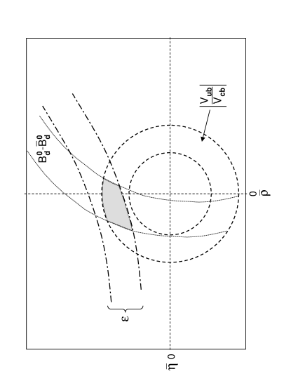
Figure 3: Schematic determination of the Unitarity Triangle.

Step 4:

From the measured $\Delta M_{d}$ that represents the $B_{d}^{0}-\bar{B}_{d}^{0}$ mixing and the box diagrams with two top quark exchanges the side $AB=R_{t}$ of the UT can be determined:

$$R_{t}=\frac{1}{\lambda}\frac{|V_{td}|}{|V_{cb}|}=0.85\cdot\left[\frac{|V_{td}|}{7.8\cdot 10^{-3}}\right]\left[\frac{0.041}{|V_{cb}|}\right],$$ (3.63)

$$|V_{td}|=7.8\cdot 10^{-3}\left[\frac{230\,{\rm MeV}}{\sqrt{\hat{B}_{B_{d}}}F_{B_{d}}}\right]\left[\frac{\Delta M_{d}}{0.50/{\rm ps}}\right]^{0.5}\sqrt{\frac{0.55}{\eta_{B}^{QCD}}}\sqrt{\frac{2.40}{S_{0}(x_{t})}}~{}.$$ (3.64)

Here $\sqrt{\hat{B}_{B_{d}}}F_{B_{d}}$ is a non-perturbative parameter and $\eta_{B}^{QCD}=0.55\pm 0.01$ the QCD correction [45, 61]. Moreover $\overline{m}_{\rm t}(m_{\rm t})=(167\pm 5)$ GeV. The constraint in the $(\bar{\varrho},\bar{\eta})$ plane coming from this step is illustrated in fig. 3.

Step 5:

The measurement of $\Delta M_{s}$ together with $\Delta M_{d}$ allows to determine $R_{t}$ in a different manner:

$$R_{t}=0.90~{}\left[\frac{\xi}{1.24}\right]\sqrt{\frac{18.4/ps}{\Delta M_{s}}}\sqrt{\frac{\Delta M_{d}}{0.50/ps}},\qquad\xi=\frac{\sqrt{\hat{B}_{B_{s}}}F_{B_{s}}}{\sqrt{\hat{B}_{B_{d}}}F_{B_{d}}}.$$ (3.65)

One should note that $m_{\rm t}$ and $|V_{cb}|$ dependences have been eliminated this way and that $\xi$ should in principle contain much smaller theoretical uncertainties than the hadronic matrix elements in $\Delta M_{d}$ and $\Delta M_{s}$ separately.

The main uncertainties in these steps originate in the theoretical uncertainties in $\hat{B}_{K}$ and $\sqrt{\hat{B}_{d}}F_{B_{d}}$ and to a lesser extent in $\xi$ [18]:

$$\hat{B}_{K}=0.86\pm 0.15,\quad\sqrt{\hat{B}_{d}}F_{B_{d}}=(235^{+33}_{-41})~{}{\rm MeV},\quad\xi=1.24\pm 0.08~{}.$$ (3.66)

Also the uncertainties due to $|V_{ub}/V_{cb}|$ in step 2 are substantial. The QCD sum rules results for the parameters in question are similar and can be found in [18]. Finally [18]

$$\Delta M_{d}=(0.503\pm 0.006)/{\rm ps},\qquad\Delta M_{s}>14.4/{\rm ps}~{}~{}{\rm at}~{}~{}95\%~{}{\rm C.L.}$$ (3.67)

3.4 The Angle $\beta$ from $B_{d}\to\psi K_{S}$

One of the highlights of the year 2002 were the considerably improved measurements of $\sin 2\beta$ by means of the time-dependent CP asymmetry

$$a_{\psi K_{S}}(t)\equiv-a_{\psi K_{S}}\sin(\Delta M_{d}t)=-\sin 2\beta\sin(\Delta M_{d}t)~{}.$$ (3.68)

The BaBar [56] and Belle [57] collaborations find

$$(\sin 2\beta)_{\psi K_{S}}=\left\{\begin{array}[]{ll}0.741\pm 0.067\,\mbox{(stat)}\pm 0.033\,\mbox{(syst)}&\mbox{(BaBar)}\\ 0.719\pm 0.074\,\mbox{(stat)}\pm 0.035\,\mbox{(syst)}&\mbox{(Belle).}\end{array}\right.$$

Combining these results with earlier measurements by CDF, ALEPH and OPAL gives the grand average [62]

$$(\sin 2\beta)_{\psi K_{S}}=0.734\pm 0.054~{}.$$ (3.69)

This is a mile stone in the field of CP violation and in the tests of the SM as we will see in a moment. Not only violation of this symmetry has been confidently established in the $B$ system, but also its size has been measured very accurately. Moreover in contrast to the five constraints listed above, the determination of the angle $\beta$ in this manner is theoretically very clean.

3.5 Unitarity Triangle 2003 (SM)

We are now in a position to combine all these constraints in order to construct the unitarity triangle and determine various quantities of interest. In this context the important issue is the error analysis of these formulae, in particular the treatment of theoretical uncertainties. In the literature the most popular are the Bayesian approach [63] and the frequentist approach [64]. For the PDG analysis see [35]. A critical comparison of these and other methods can be found in [18]. I can recommend this reading.

In fig. 4 we show the result of the recent update of an analysis in collaboration with Parodi and Stocchi [55] that uses the Bayesian approach. The allowed region for $(\bar{\varrho},\bar{\eta})$ is the area inside the smaller ellipse. We observe that the region $\bar{\varrho}<0$ is disfavoured by the lower bound on $\Delta M_{s}$. It is clear from this figure that the measurement of $\Delta M_{s}$ giving $R_{t}$ through (3.65) will have a large impact on the plot in fig. 4.

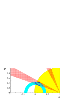
Figure 4: The allowed 95$\%$ regions in the $(\bar{\varrho},\bar{\eta})$ plane in the SM (narrower region) and in the MFV models (broader region) from the update of [55]. The individual 95$\%$ regions for the constraint from $\sin 2\beta$, $\Delta M_{s}$ and $R_{b}$ are also shown.

The ranges for various quantities that result from this analysis are given in the SM column of table 1. The UUT column will be discussed soon. The SM results follow from the five steps listed above and (3.69) implying an impressive precision on the angle $\beta$:

$$(\sin 2\beta)_{\rm tot}=0.705^{+0.042}_{-0.032},\qquad\beta=(22.4\pm 1.5)^{\circ}~{}.$$ (3.70)

On the other hand $(\sin 2\beta)_{ind}$ obtained by means of the five steps only is found to be [55]

$$(\sin 2\beta)_{ind}=0.685\pm 0.052,$$ (3.71)

demonstrating an excellent agreement (see also fig. 4) between the direct measurement in (3.69) and the standard analysis of the UT within the SM. This gives a strong indication that the CKM matrix is very likely the dominant source of CP violation in flavour violating decays and gives a support to the MFV idea. In order to be sure whether this is indeed the case, other theoretically clean quantities have to be measured. In particular the angle $\gamma$ that is more sensitive to new physics contributions than $\beta$. We refer to [12] and [22] for reviews of the methods relevant for this determination.

Table 1: Values for different quantities from the update of [55]. $\lambda_{t}=V_{ts}^{*}V_{td}$.

Strategy	UUT	SM
$\bar{\eta}$	0.361 $\pm$ 0.032	0.341 $\pm$ 0.028
$\bar{\varrho}$	0.149 $\pm$ 0.056	0.178 $\pm$ 0.046
$\sin 2\beta$	0.715 ${}^{+0.037}_{-0.034}$	0.705 ${}^{+0.042}_{-0.032}$
$\sin 2\alpha$	0.03 $\pm$ 0.31	–0.19 $\pm$ 0.25
$\gamma$	$(67.5\pm 8.9)^{\circ}$	$(61.5\pm 7.0)^{\circ}$
$R_{b}$	0.393 $\pm$ 0.025	0.390 $\pm$ 0.024
$R_{t}$	$0.925\pm 0.060$	$0.890\pm 0.048$
$\Delta M_{s}$ ($ps^{-1}$)	17.3${}^{+2.1}_{-1.3}$	18.3${}^{+1.7}_{-1.5}$
$|V_{td}|~{}(10^{-3})$	8.61 $\pm$ 0.55	8.24 $\pm$ 0.41
${\rm Im}\lambda_{t}$ ($10^{-4}$)	1.39 $\pm$ 0.12	1.31 $\pm$ 0.10

3.6 Unitarity Triangle 2003 (MFV)

In a general MFV model the formulae (3.60)–(3.69) still apply with $S_{0}(x_{t})$ replaced by the master function $S(v)$. In particular as emphasized in [65], $S(v)$ could be negative resulting in $\bar{\eta}<0$. As found in [65, 7] this case is disfavoured but not yet excluded. Here we will only consider $S(v)>0$. We recall that in the absence of new CP violating phases, (3.69) determines a universal angle $\beta$ in the MFV models. Moreover we note that not only (3.69) but also (3.60), (3.61) and (3.65) do not involve $S(v)$ and are universal within the MFV models. Using only them allows to construct a universal unitarity triangle (UUT) common to all these models [6]. The apex of the UUT is positioned within the larger ellipse in figure 4 as obtained recently in an update of [55]. The results for various quantities of interest related to this UUT are collected in table 1. A similar analysis has been done in [7].

It should be stressed that any MFV model that is inconsistent with the broader allowed region in figure 4 and the UUT column in table 1 is ruled out. We observe that there is little room for MFV models that in their predictions for UT differ significantly from the SM. It is also clear that to distinguish the SM from the MFV models on the basis of the analysis of the UT presented above, will require considerable reduction of theoretical uncertainties. Therefore for the near future the most precise determination of the UUT will come from $\sin 2\beta$ measured through $a_{\psi K_{S}}$ and the ratio $\Delta M_{s}/\Delta M_{d}$ as advocated in Section 3.2.

4 Relations from Minimal Flavour Violation

4.1 Preliminaries

We have seen that an UUT could be constructed. In this construction the relation between $R_{t}$ and the ratio $\Delta M_{d}/\Delta M_{s}$, that does not depend on $F_{r}$, played an important role. It is clear from the tables in Sections 2.5 and 2.8 that there are other interesting relations between branching ratios and various observables which similarly to UUT are independent of $F_{r}$. These relations are very important for testing the general concept of MFV. In order to illuminate the origin of the MFV relations in question we will now list the formulae for most important decays in the MFV models. Because of space limitations our presentation will be reduced to the minimum. Details on these formulae can be found in [13, 15, 40, 41] and references therein. The numerical constants in the formulae below correspond to [35] and

$$\sin^{2}\theta_{w}=0.231,\qquad\alpha=\frac{1}{128},\qquad\lambda=0.224$$ (4.72)

with the first two given in the $\overline{MS}$ scheme. They differ slightly from those in [13, 15, 40, 41].

4.2 Basic Formulae

4.2.1 The $\varepsilon_{K}$ Constraint

Similarly to (3.62) we have

$$\bar{\eta}\left[(1-\bar{\varrho})A^{2}\eta^{QCD}_{2}S(v)+P_{c}(\varepsilon)\right]A^{2}\hat{B}_{K}=0.187,$$ (4.73)

where $P_{c}(\varepsilon)=0.29\pm 0.07$ and $\eta^{QCD}_{2}=0.57\pm 0.01$ as before.

4.2.2 $B^{0}_{d,s}-\bar{B}^{0}_{d,s}$ Mixing

Within the MFV models $\Delta M_{s,d}$ are given as follows ($q=d,s$) [16]

$$\Delta M_{q}=\frac{G_{\rm F}^{2}}{6\pi^{2}}\eta_{B}^{QCD}m_{B_{q}}(\hat{B}_{q}F_{B_{q}}^{2})M_{\rm W}^{2}|V^{\ast}_{tb}V_{tq}|^{2}S(v),$$ (4.74)

where $\eta_{B}^{QCD}=0.55\pm 0.01$ [45, 61], impling (3.63)–(3.65) with $S_{0}(x_{t})$ in (3.64) replaced by $S(v)$.

4.2.3 $K\to\pi\nu\bar{\nu}$

The rare decays $K^{+}\rightarrow\pi^{+}\nu\bar{\nu}$ and $K_{\rm L}\rightarrow\pi^{0}\nu\bar{\nu}$ proceed through $Z^{0}$-penguin and box diagrams. As the required hadronic matrix elements can be extracted from the leading semileptonic decays and other long distance contributions turn out to be negligible [66], the relevant branching ratios can be computed to an exceptionally high degree of precision [46, 47, 48].

The basic formulae for the branching ratios are given in MFV as follows

$$Br(K^{+}\rightarrow\pi^{+}\nu\bar{\nu})=4.78\cdot 10^{-11}\cdot\left[\left({\rm Im}F_{t}\right)^{2}+\left({\rm Re}F_{c}+{\rm Re}F_{t}\right)^{2}\right]~{},$$ (4.75)

$$Br(K_{\rm L}\to\pi^{0}\nu\bar{\nu})=2.09\cdot 10^{-10}\cdot\left({\rm Im}F_{t}\right)^{2}~{},$$ (4.76)

where

$$F_{c}={\lambda_{c}\over\lambda}P_{c}(X),\qquad F_{t}={\lambda_{t}\over\lambda^{5}}X(v),\qquad\lambda_{i}=V^{\ast}_{is}V_{id}$$ (4.77)

and $P_{c}(X)=0.39\pm 0.06$ results from the internal charm contribution [46, 47].

Imposing all existing constraints on the CKM matrix one finds [66, 67]

$$Br(K^{+}\rightarrow\pi^{+}\nu\bar{\nu})=(7.7\pm 1.1)\cdot 10^{-11},\qquad Br(K_{\rm L}\rightarrow\pi^{0}\nu\bar{\nu})=(2.6\pm 0.5)\cdot 10^{-11}$$ (4.78)

where the errors come dominantly from the uncertainties in the CKM parameters. This should be compared respectively with the results of AGS E787 collaboration [68] and KTeV [69]

$$Br(K^{+}\rightarrow\pi^{+}\nu\bar{\nu})=(15.7^{+17.5}_{-8.2})\cdot 10^{-11},\qquad Br(K_{\rm L}\rightarrow\pi^{0}\nu\bar{\nu})<5.9\cdot 10^{-7}\,.$$ (4.79)

4.2.4 $B\to X_{s,d}\nu\bar{\nu}$

Theoretically clean [46, 70] are also the inclusive decays $B\to X_{s,d}\nu\bar{\nu}$ for which the branching ratios read

$$Br(B\to X_{q}\nu\bar{\nu})=1.58\cdot 10^{-5}\left[\frac{Br(B\to X_{c}e\bar{\nu})}{0.104}\right]\left[\frac{0.54}{f(z)}\right]\frac{|V_{tq}|^{2}}{|V_{cb}|^{2}}X^{2}(v)$$ (4.80)

where $f(z)$ is a phase space factor for $B\to X_{c}e\bar{\nu}$. The SM expectation

$$Br(B\to X_{s}\nu\bar{\nu})=(3.5\pm 0.5)\cdot 10^{-5}$$ (4.81)

is to be compared with the $90\%$ C.L ALEPH upper bound $6.4\cdot 10^{-4}$. The exclusive channels are less clean but experimentally easier accessible with the $90\%$ C.L BaBar upper bound of $7.0\cdot 10^{-5}$.

4.2.5 $K_{L}\to\mu^{+}\mu^{-}$

The short distance contribution to the dispersive part of $K_{\rm L}\to\mu^{+}\mu^{-}$ is given by [46, 47]

$$Br(K_{\rm L}\to\mu^{+}\mu^{-})_{\rm SD}=1.95\cdot 10^{-9}\left[\frac{{\rm Re}\lambda_{c}}{\lambda}P_{c}(Y)+\frac{{\rm Re}\lambda_{t}}{\lambda^{5}}Y(v)\right]^{2},$$ (4.82)

where $P_{c}(Y)=0.121\pm 0.012$ [47]. Unfortunately due to long distance contributions to the dispersive part of $K_{L}\to\mu^{+}\mu^{-}$, the extraction of $Br(K_{\rm L}\to\mu^{+}\mu^{-})_{\rm SD}$ from the data is subject to considerable uncertainties [71, 72]. While the chapter on this extraction is certainly not closed, let us quote the estimate of [71] that reads

$$Br(K_{\rm L}\to\mu^{+}\mu^{-})_{\rm SD}\leq 2.5\cdot 10^{-9}~{}$$ (4.83)

to be compared with $Br(K_{\rm L}\to\mu^{+}\mu^{-})_{\rm SD}=(0.8\pm 0.3)\cdot 10^{-9}$ in the SM.

On the other hand the parity violating muon polarization asymmetry $\Delta_{\rm LR}$ in $K^{+}\to\pi^{+}\mu^{+}\mu^{-}$ is substantially cleaner [73]. It is given at NLO level by [74]

$$|\Delta_{\rm LR}|=r\cdot 1.78\cdot 10^{-3}\left|\frac{{\rm Re}\lambda_{c}}{\lambda}P_{c}(Y)+\frac{{\rm Re}\lambda_{t}}{\lambda^{5}}Y(v)\right|,$$ (4.84)

where $r$ is a phase factor that may depend on various experimental cuts.

4.2.6 $B_{q}\to\mu\bar{\mu}$

Next, the branching ratios for the rare decays $B_{q}\to\mu^{+}\mu^{-}$ are given by

$$Br(B_{q}\to\mu^{+}\mu^{-})=\tau(B_{q})\frac{G^{2}_{\rm F}}{\pi}\eta_{Y}^{2}\left(\frac{\alpha}{4\pi\sin^{2}\theta_{W}}\right)^{2}F^{2}_{B_{q}}m^{2}_{\mu}m_{B_{q}}|V^{\ast}_{tb}V_{tq}|^{2}Y^{2}(v),$$ (4.85)

where $\eta_{Y}=1.012$ [47] are the short distance QCD corrections evaluated using $m_{t}\equiv\overline{m}_{t}(m_{t})$. In writing (4.85) we have neglected the terms ${\cal O}(m_{\mu}^{2}/m_{B_{q}}^{2})$ in the phase space factor. In the SM one finds [75] (see Section 4.4)

$$Br(B_{s}\to\mu\bar{\mu})=(3.42\pm 0.54)\cdot 10^{-9},\qquad Br(B_{d}\to\mu\bar{\mu})=(1.00\pm 0.14)\cdot 10^{-10}$$ (4.86)

where to reduce the hadronic uncertainties the experimental data for $\Delta M_{d}$ and as an example $\Delta M_{s}=(18.0\pm 0.5)/{\rm ps}$ have been used. This should be compared respectively with the $90\%$ C.L. bounds from CDF(D0) and Belle [76, 77]

$$Br(B_{s}\to\mu\bar{\mu})<9.5~{}(16)\cdot 10^{-7},\qquad Br(B_{d}\to\mu\bar{\mu})<1.6\cdot 10^{-7}.$$ (4.87)

4.2.7 $K_{L}\to\pi^{0}e^{+}e^{-}$

The rare decay $K_{L}\to\pi^{0}e^{+}e^{-}$ is dominated by CP-violating contributions. It has been recently reconsidered within the SM [78] in view of the most recent NA48 data on $K_{S}\to\pi^{0}e^{+}e^{-}$ and $K_{L}\to\pi^{0}\gamma\gamma$ [79] that allow a much better evaluation of the indirectly (mixing) CP-violating and CP-conserving contributions. The directly CP-violating contribution has been know already at NLO for some time [80]. The CP-conserving part is found to be below $3\cdot 10^{-12}$ [78].

Generalizing the formula (33) in [78] to MFV models we obtain

$$Br(K_{\rm L}\to\pi^{0}e^{+}e^{-})_{\rm CPV}=10^{-12}\cdot\left[C_{\rm mix}+C_{\rm int}\left(\frac{{\rm Im}\lambda_{t}}{10^{-4}}\right)+C_{\rm dir}\left(\frac{{\rm Im}\lambda_{t}}{10^{-4}}\right)^{2}\right],$$ (4.88)

where

$$C_{\rm mix}=(15.7\pm 0.3)|a_{s}|^{2},\qquad|a_{s}|=1.08^{+0.26}_{-0.21},$$ (4.89)

$$C_{\rm dir}=6.2\cdot 10^{-2}(\tilde{y}_{7A}^{2}+\tilde{y}_{7V}^{2})\,,\qquad C_{\rm int}=0.34\,\tilde{y}_{7V}\,\sqrt{C_{\rm mix}}.$$ (4.90)

Here

$$\tilde{y}_{7V}=P_{0}+\frac{Y(v)}{\sin^{2}\theta_{w}}-4Z(v)+P_{E}E(v)~{},\qquad\tilde{y}_{7A}=-\frac{1}{\sin^{2}\theta_{w}}Y(v),$$ (4.91)

where ${\rm Im}\lambda_{t}={\rm Im}(V_{td}V^{*}_{ts})$, $P_{0}=2.89\pm 0.06$ [80] and $P_{E}$ is ${\cal O}(10^{-2})$. Consequently the last term in $\tilde{y}_{7V}$ can be neglected. The effect of new physics contributions is mainly felt in $\tilde{y}_{7A}$ as the corresponding contributions in $\tilde{y}_{7V}$ cancel each other to a large extent.

The present experimental bound from KTeV [81]

$$Br(K_{\rm L}\to\pi^{0}e^{+}e^{-})<2.8\cdot 10^{-10}\qquad(90\%{\rm C.L.})$$ (4.92)

should be compared with the SM prediction [78]

$$Br(K_{\rm L}\to\pi^{0}e^{+}e^{-})_{\rm SM}=(3.2^{+1.2}_{-0.8})\cdot 10^{-11}~{}.$$ (4.93)

4.2.8 $\varepsilon^{\prime}/\varepsilon$

The formula for the CP-violating ratio $\varepsilon^{\prime}/\varepsilon$ of [82] generalizes to the arbitrary MFV model as follows:

$$\frac{\varepsilon^{\prime}}{\varepsilon}={\rm Im}\lambda_{t}\cdot F_{\varepsilon^{\prime}}(v)$$ (4.94)

where

$$F_{\varepsilon^{\prime}}(v)=P_{0}+P_{X}\,X(v)+P_{Y}\,Y(v)+P_{Z}\,Z(v)+P_{E}\,E(v)~{}.$$ (4.95)

The numerical values of the coefficients $P_{i}$ can be found in [82]. They depend strongly on the hadronic matrix elements of the relevant operators and the value of $\alpha_{s}$. For instance for the non-perturbative parameters $R_{6}=1.2$ and $R_{8}=1.0$ in [82] and $\alpha_{s}(M_{Z})=0.119$ one has

$$P_{0}=19.5,\qquad P_{X}=0.6,\qquad P_{Y}=0.5,\qquad P_{Z}=-12.4,\qquad P_{E}=-1.6$$ (4.96)

with $P_{0}$ and $P_{Z}$ originating dominantly in the matrix elements of the QCD penguin $Q_{6}$ and the electroweak penguin $Q_{8}$, respectively. On the other for $R_{6}=1.6$, $R_{8}=0.8$ and $\alpha_{s}(M_{Z})=0.121$ one has

$$P_{0}=28.6,\qquad P_{X}=0.6,\qquad P_{Y}=0.6,\qquad P_{Z}=-10.3,\qquad P_{E}=-2.7~{}.$$ (4.97)

On the experimental side the world average based on the latest results from NA48 [83] and KTeV [84], and previous results from NA31 and E731, reads

$$\varepsilon^{\prime}/\varepsilon=(16.6\pm 1.6)\cdot 10^{-4}\qquad\qquad(2003)~{}.$$ (4.98)

While several analyses of recent years within the SM find results that are compatible with (4.98) it is fair to say, in view of large hadronic uncertainties in the coefficients $P_{i}$, that the chapter on the theoretical calculations of $\varepsilon^{\prime}/\varepsilon$ is far from being closed. For instance with $m_{t}=167\,{\rm GeV}$ and ${\rm Im}\lambda_{t}=1.44\cdot 10^{-4}$ (see an example in Section 5.5) one finds in the SM $\varepsilon^{\prime}/\varepsilon=17.4\cdot 10^{-4}$ and $32.2\cdot 10^{-4}$ for (4.96) and (4.97), respectively. The most recent analysis with the relevant references is given in [82].

4.2.9 $B\to X_{s}\gamma$ and $B\to X_{s}~{}{\rm gluon}$

These decays are governed by the magnetic–penguin operators

$$Q_{7\gamma}=\frac{e}{8\pi^{2}}m_{b}\bar{s}_{\alpha}\sigma^{\mu\nu}(1+\gamma_{5})b_{\alpha}F_{\mu\nu},\qquad Q_{8G}=\frac{g_{s}}{8\pi^{2}}m_{b}\bar{s}_{\alpha}\sigma^{\mu\nu}(1+\gamma_{5})T^{a}_{\alpha\beta}b_{\beta}G^{a}_{\mu\nu}$$ (4.99)

originating in the diagrams of fig. 2d with an on-shell photon and gluon, respectively. Their Wilson coefficients are strongly affected by QCD corrections [85, 86] coming dominantly from the mixing of $Q_{7\gamma}$ and $Q_{8G}$ with current–current operators.

In the leading logarithmic approximation one has

$${Br(B\to X_{s}\gamma)}=2.88\cdot 10^{-3}\left[\frac{Br(B\to X_{c}e\bar{\nu})}{0.104}\right]\left[\frac{0.54}{f(z)}\right]\frac{|V_{ts}|^{2}}{|V_{cb}|^{2}}|C^{(0){\rm eff}}_{7}(\mu_{b})|^{2}\,,$$ (4.100)

where $f(z)$ is the phase space factor in $Br(B\to X_{c}e\bar{\nu}_{e})$. The Wilson coefficient $C^{(0){\rm eff}}_{7}(\mu_{b})$ is given by

$$C^{(0){\rm eff}}_{7\gamma}(\mu_{b})=-0.348\,D^{\prime}(v)-0.042\,E^{\prime}(v)-0.158$$ (4.101)

where we have set $\mu_{b}=5\,{\rm GeV}$ and $\alpha_{s}^{(5)}(M_{\rm Z})=0.118$. The last term in this formula comes from the mixing with the current–current operator $Q_{2}$ and the coefficients in front of the master functions come from the renormalization group analysis. The small coefficient in front of $E^{\prime}(v)$ makes this function subleading in this decay.

The corresponding NLO formulae that include also higher order electroweak effects [87] are very complicated and can be found in [88]. As reviewed in [89, 90, 91], many groups contributed to obtain these NLO results, in particular Christoph Greub, Mikolaj Misiak and their collaborators. See also [92].

On the experimental side the world average resulting from the data by CLEO, ALEPH, BaBar and Belle reads [18]

$$Br(B\to X_{s}\gamma)_{E_{\gamma}>1.6{\rm GeV}}=(3.28^{+0.41}_{-0.36})\cdot 10^{-4}~{}.$$ (4.102)

It agrees well with the SM result [88]

$$Br(B\to X_{s}\gamma)^{\rm{SM}}_{E_{\gamma}>1.6{\rm GeV}}=(3.57\pm 0.30)\cdot 10^{-4}~{}.$$ (4.103)

The $B\to X_{s}~{}{\rm gluon}$ decay is dominated by $Q_{8G}$ with $C^{(0){\rm eff}}_{8G}$ given by

$$C^{(0){\rm eff}}_{8G}(\mu_{b})=-0.364\,E^{\prime}(v)-0.074$$ (4.104)

with the last term representing QCD renormalization group effect. The NLO corrections have been calculated in [93]. Unfortunately, the remaining strong renormalization scale dependence in the resulting branching ratio and the difficulty in extracting it from the experiment, make these results not yet useful at present.

4.2.10 $B\to X_{s}\mu^{+}\mu^{-}$ and $A_{FB}(\hat{s})$

This decay is dominated by the operators

$$Q_{9V}=(\bar{s}b)_{V-A}(\bar{\mu}\mu)_{V}\,,\qquad Q_{10A}=(\bar{s}b)_{V-A}(\bar{\mu}\mu)_{A}\,.$$ (4.105)

They are generated through the electroweak penguin diagrams of fig. 2f and the related box diagrams are needed mainly to keep gauge invariance. At low

$$\hat{s}=\frac{(p_{\mu^{+}}+p_{\mu^{-}})^{2}}{m_{\rm b}^{2}},$$ (4.106)

also the magnetic operator $Q_{7\gamma}$ plays a significant role.

At the NLO level [94, 95] the invariant dilepton mass spectrum is given by

$$\frac{{d}/{d\hat{s}}\,\Gamma(b\to s\mu^{+}\mu^{-})}{\Gamma(b\to ce\bar{\nu})}=\frac{\alpha^{2}}{4\pi^{2}}\left|\frac{V_{ts}}{V_{cb}}\right|^{2}\frac{(1-\hat{s})^{2}}{f(z)\kappa(z)}U(\hat{s})$$ (4.107)

where

$$U(\hat{s})=(1+2\hat{s})\left(|\tilde{C}_{9}^{\rm eff}(\hat{s})|^{2}+|\tilde{C}_{10}|^{2}\right)+4\left(1+\frac{2}{\hat{s}}\right)|C_{7\gamma}^{(0){\rm eff}}|^{2}+12C_{7\gamma}^{(0){\rm eff}}\ {\rm Re}\,\tilde{C}_{9}^{\rm eff}(\hat{s})$$ (4.108)

and $\tilde{C}_{9}^{\rm eff}(\hat{s})$ is a function of $\hat{s}$ that depends on the Wilson coefficient $\tilde{C}_{9}$ and includes also contributions from four quark operators. Explicit formula can be found in [94, 95].

The Wilson coefficients $\tilde{C}_{9}$ and $\tilde{C}_{10}$ are given as follows

$$\tilde{C}_{9}(\mu)=P_{0}+\frac{Y(v)}{\sin^{2}\theta_{w}}-4Z(v)+P_{E}E(v),\qquad\tilde{C}_{10}(\mu)=-\frac{Y(v)}{\sin^{2}\theta_{w}}$$ (4.109)

with $P_{0}=2.60\pm 0.25$ in the NDR scheme and $P_{E}={\cal O}(10^{-2})$. Note the great similarity to (4.91). $\tilde{C}_{9}$ and $\tilde{C}_{10}$ are defined by

$$C_{9V}(\mu)=\frac{\alpha}{2\pi}\tilde{C}_{9}(\mu),\qquad C_{10A}(\mu)=\frac{\alpha}{2\pi}\tilde{C}_{10}(\mu).$$ (4.110)

Of particular interest is the Forward-Backward asymmetry in $B\to X_{s}\mu^{+}\mu^{-}$. It becomes non-zero only at the NLO level and is given in this approximation by [96]

$$A_{\rm FB}(\hat{s})=-3\tilde{C}_{10}\frac{\left[\hat{s}{\rm Re}\,\tilde{C}_{9}^{\rm eff}(\hat{s})+2C_{7\gamma}^{(0){\rm eff}}\right]}{U(\hat{s})}$$ (4.111)

with $U(\hat{s})$ given in (4.108). Similar to the case of exclusive decays [97], the asymmetry $A_{\rm FB}(\hat{s})$ vanishes at $\hat{s}=\hat{s}_{0}$ that in the case of the inclusive decay considered is determined through

$$\hat{s}_{0}{\rm Re}\,\tilde{C}_{9}^{\rm eff}(\hat{s}_{0})+2C_{7\gamma}^{(0){\rm eff}}=0.$$ (4.112)

$A_{\rm FB}(\hat{s})$ and the value of $\hat{s}_{0}$ are sensitive to short distance physics and subject to only very small non-perturbative uncertainties. Consequently, they are particularly useful quantities to test the physics beyond the SM.

The calculations of $A_{\rm FB}(\hat{s})$ and of $\hat{s}_{0}$ in the SM have recently been done including NNLO corrections [98, 99] that turn out to be significant. In particular they shift the NLO value of $\hat{s}_{0}$ from $0.142$ to $0.162$ at NNLO.

The most recent reviews summarizing the theoretical status can be found in [91, 28]. On the experimental side the Belle and BaBar collaborations [100] reported the observation of this decay and of the $X_{s}e^{+}e^{-}$ channel. The $90\%$ C.L. ranges extracted from these papers [101] read

$$3.5\cdot 10^{-6}\leq Br(B\to X_{s}\mu^{+}\mu^{-})\leq 10.4\cdot 10^{-6}~{},$$ (4.113)

$$2.8\cdot 10^{-6}\leq Br(B\to X_{s}\mu^{+}\mu^{-})\leq 8.8\cdot 10^{-6}.$$ (4.114)

4.3 Model Independent Relations

We will now list a number of relations between various observables that do not depend on the functions $F_{r}(v)$ and consequently are universal within the class of MFV models.

1. From (4.74), (4.80) and (4.85) we find [29]

$$\frac{\Delta M_{d}}{\Delta M_{s}}=\frac{m_{B_{d}}}{m_{B_{s}}}\frac{\hat{B}_{d}}{\hat{B}_{s}}\frac{F^{2}_{B_{d}}}{F^{2}_{B_{s}}}\left|\frac{V_{td}}{V_{ts}}\right|^{2}$$ (4.115)

$$\frac{Br(B\to X_{d}\nu\bar{\nu})}{Br(B\to X_{s}\nu\bar{\nu})}=\left|\frac{V_{td}}{V_{ts}}\right|^{2}$$ (4.116)

$$\frac{Br(B_{d}\to\mu^{+}\mu^{-})}{Br(B_{s}\to\mu^{+}\mu^{-})}=\frac{\tau({B_{d}})}{\tau({B_{s}})}\frac{m_{B_{d}}}{m_{B_{s}}}\frac{F^{2}_{B_{d}}}{F^{2}_{B_{s}}}\left|\frac{V_{td}}{V_{ts}}\right|^{2}$$ (4.117)

that all can be used to determine $|V_{td}/V_{ts}|$ without the knowledge of $F_{r}(v)$ [6]. In particular, as already emphasized in Section 3, the relation (4.115) will offer after the measurement of $\Delta M_{s}$ a powerful determination of the length of one side of the unitarity triangle, denoted usually by $R_{t}$.

Out of these three ratios the cleanest is (4.116), which is essentially free of hadronic uncertainties [70]. Next comes (4.117), involving $SU(3)$ breaking effects in the ratio of $B$-meson decay constants. Finally, $SU(3)$ breaking in the ratio $\hat{B}_{B_{d}}/\hat{B}_{B_{s}}$ enters in addition in (4.115). These $SU(3)$ breaking effects should eventually be calculable with high precision from lattice QCD.

Eliminating $|V_{td}/V_{ts}|$ from the three relations above allows to obtain three relations between observables that are universal within the MFV models. In particular from (4.115) and (4.117) one finds [75]

$$\frac{Br(B_{s}\to\mu\bar{\mu})}{Br(B_{d}\to\mu\bar{\mu})}=\frac{\hat{B}_{d}}{\hat{B}_{s}}\frac{\tau(B_{s})}{\tau(B_{d})}\frac{\Delta M_{s}}{\Delta M_{d}},$$ (4.118)

that does not involve $F_{B_{q}}$ and consequently contains substantially smaller hadronic uncertainties than the formulae considered above. It involves only measurable quantities except for the ratio $\hat{B}_{s}/\hat{B}_{d}$ that is known already now from lattice calculations with respectable precision [18]:

$$\frac{\hat{B}_{s}}{\hat{B}_{d}}=1.00\pm 0.03,\qquad\hat{B}_{d}=1.34\pm 0.12,\qquad\hat{B}_{s}=1.34\pm 0.12~{}.$$ (4.119)

With the future precise measurement of $\Delta M_{s}$, the formula (4.118) will give a very precise prediction for the ratio of the branching ratios $Br(B_{q}\to\mu\bar{\mu})$.

2. Next, combining (4.75) and (4.76), it is possible to derive a very accurate formula for $\sin 2\beta$ that depends only on the $K\to\pi\nu\bar{\nu}$ branching ratios and $P_{c}(X)$ [29]:

$$\sin 2\beta=\frac{2r_{s}}{1+r_{s}^{2}},\qquad r_{s}=\sqrt{\sigma}{\sqrt{\sigma(B_{1}-B_{2})}-P_{c}(X)\over\sqrt{B_{2}}}\,,$$ (4.120)

where $\sigma=1/(1-\lambda^{2}/2)^{2}$ and we have assumed $X>0$. The corresponding formula valid also for $X<0$ is given in [65]. Here we have defined the “reduced” branching ratios

$$B_{1}={Br(K^{+}\rightarrow\pi^{+}\nu\bar{\nu})\over 4.78\cdot 10^{-11}},\qquad B_{2}={Br(K_{\rm L}\rightarrow\pi^{0}\nu\bar{\nu})\over 2.09\cdot 10^{-10}}.$$ (4.121)

It should be stressed that $\sin 2\beta$ determined this way depends only on two measurable branching ratios and on $P_{c}(X)$ which is completely calculable in perturbation theory. Consequently this determination is free from any hadronic uncertainties and its accuracy can be estimated with a high degree of confidence. With measurements of $Br(K^{+}\rightarrow\pi^{+}\nu\bar{\nu})$ and $Br(K_{\rm L}\rightarrow\pi^{0}\nu\bar{\nu})$ with $10\%$ accuracy a determination of $\sin 2\beta$ with an error of $0.05$ is possible.

Moreover, as in MFV models there are no phases beyond the CKM phase, we also expect

$$(\sin 2\beta)_{\pi\nu\bar{\nu}}=(\sin 2\beta)_{J/\psi K_{S}},\qquad(\sin 2\beta)_{\phi K_{S}}\approx(\sin 2\beta)_{J/\psi K_{S}}.$$ (4.122)

with the accuracy of the last relation at the level of a few percent [102]. The confirmation of these two relations would be a very important test for the MFV idea. Indeed, in $K\to\pi\nu\bar{\nu}$ the phase $\beta$ originates in the $Z^{0}$ penguin diagram, whereas in the case of $a_{J/\psi K_{S}}$ in the $B^{0}_{d}-\bar{B}^{0}_{d}$ box diagram. In the case of the asymmetry $a_{J/\phi K_{S}}$ it originates also in $B^{0}_{d}-\bar{B}^{0}_{d}$ box diagrams but the second relation in (4.122) could be spoiled by new physics contributions in the decay amplitude for $B\to\phi K_{S}$ that is non-vanishing only at the one loop level.

An important consequence of (4.120) and (4.122) is the following one. For a given $\sin 2\beta$ extracted from $a_{J/\psi K_{S}}$ and $Br(K^{+}\rightarrow\pi^{+}\nu\bar{\nu})$ only two values of $Br(K_{\rm L}\rightarrow\pi^{0}\nu\bar{\nu})$, corresponding to two signs of $X$, are possible in the full class of MFV models, independent of any new parameters present in these models [65]. Consequently, measuring $Br(K_{\rm L}\rightarrow\pi^{0}\nu\bar{\nu})$ will either select one of these two possible values or rule out all MFV models. The present experimental bound on $Br(K^{+}\rightarrow\pi^{+}\nu\bar{\nu})$ and $\sin 2\beta\leq 0.80$ imply in this manner an absolute upper bound $Br(K_{\rm L}\rightarrow\pi^{0}\nu\bar{\nu})<4.9\cdot 10^{-10}~{}(90\%~{}{\rm C.L.})$ [65] in the MFV models that is by a factor of three stronger than the model independent bound [103] from isospin symmetry. However, as we will see in Section 5.5, even stronger bound on $Br(K_{\rm L}\rightarrow\pi^{0}\nu\bar{\nu})$ can be obtained once the data on $B\to X_{s}\mu^{+}\mu^{-}$ are taken into account.

3. It turns out that in most MFV models the coefficient $C_{9V}$ is only very weakly dependent on new physics contributions. Consequently, as pointed out in [41], a correlation between $\hat{s}_{0}$ in $A_{\rm FB}$ and $Br(B\to X_{s}\gamma)$ exists. It is present in the ACD model discussed in Section 6 and in a large class of supersymmetric models discussed for instance in [28]. We show this correlation in fig. 5.

\psfragscanon\psfrag{bsgammabsgammabsgamma}{ \shortstack{\\ \\ $(Br(B\to X_{s}\gamma)\times 10^{4})^{\frac{1}{2}}$ ${}$}}\psfrag{hats0}{ \shortstack{\\ $\hat{s}_{0}$ }}\includegraphics{corr.eps}

Figure 5: Correlation between $\sqrt{Br(B\to X_{s}\gamma)}$ and $\hat{s}_{0}$ [41]. The dots are the results in the ACD model (see Section 6) for $1/R=200,250,300,350,400,600$ and $1000$ GeV and the star denotes the SM value.

4. Very recently a correlation between the $B\to\pi K$ modes and $Br(K^{+}\rightarrow\pi^{+}\nu\bar{\nu})$ in a MFV new-physics scenario with enhanced $Z^{0}$ penguins has been pointed out in [58]. In fig. 6 we show $Br(K^{+}\rightarrow\pi^{+}\nu\bar{\nu})$ as a function of the variable $\bar{L}$ that is given entirely in terms of $B\to\pi K$ observables and $|V_{ub}/V_{cb}|$. For a general discussion of correlations between $B\to\pi K$ decays and rare decays we refer to [58].

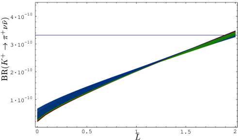
Figure 6: Correlation between $Br(K^{+}\rightarrow\pi^{+}\nu\bar{\nu})$ and the $B\to\pi K$ variable $\bar{L}$.

5. Other correlations between various decays can be found in [104, 53, 105, 65, 106]. For instance there exists in addition to an obvious correlation between $K\to\pi\nu\bar{\nu}$ and $B\to X_{q}\nu\bar{\nu}$ also a correlation between $\varepsilon^{\prime}/\varepsilon$ and rare semileptonic $B$ and $K$ decays.

4.4 Model Dependent Relations

4.4.1 $B_{q}\to\mu\bar{\mu}$ and $\Delta M_{q}$

From (4.74) and (4.85) we derive [75]

$$Br(B_{q}\to\mu\bar{\mu})=4.36\cdot 10^{-10}\frac{\tau(B_{q})}{\hat{B}_{q}}\frac{Y^{2}(v)}{S(v)}\Delta M_{q},\qquad(q=s,d).$$ (4.123)

These relations allow to predict $Br(B_{s,d}\to\mu\bar{\mu})$ in a given MFV model with substantially smaller hadronic uncertainties than found by using directly the formulae in (4.85). In particular using the formulae for the functions $Y$ and $S$ in the SM model of Section 2.5, we find [75]

$$Br(B_{s}\to\mu\bar{\mu})=3.42\cdot 10^{-9}\left[\frac{\tau(B_{s})}{1.46~{}{\rm ps}}\right]\left[\frac{1.34}{\hat{B}_{s}}\right]\left[\frac{\overline{m}_{t}(m_{t})}{167\,{\rm GeV}}\right]^{1.6}\left[\frac{\Delta M_{s}}{18.0/{\rm ps}}\right],$$ (4.124)

$$Br(B_{d}\to\mu\bar{\mu})=1.00\cdot 10^{-10}\left[\frac{\tau(B_{d})}{1.54~{}{\rm ps}}\right]\left[\frac{1.34}{\hat{B}_{d}}\right]\left[\frac{\overline{m}_{t}(m_{t})}{167\,{\rm GeV}}\right]^{1.6}\left[\frac{\Delta M_{d}}{0.50/{\rm ps}}\right].$$ (4.125)

Using $\overline{m}_{t}(m_{t})=(167\pm 5)\,{\rm GeV}$, the lifetimes from [18], $\hat{B}_{q}$ in (4.119), $\Delta M_{d}=(0.503\pm 0.006)/{\rm ps}$ and taking as an example $\Delta M_{s}=(18.0\pm 0.5)/{\rm ps}$, we find the predictions for the branching ratios in question given in (4.86). They are substantially more accurate than the ones found in the literature in the past.

4.4.2 $Br(K^{+}\rightarrow\pi^{+}\nu\bar{\nu})$, $\Delta M_{d}/\Delta M_{s}$ and $\beta$.

In [47] an upper bound on $Br(K^{+}\rightarrow\pi^{+}\nu\bar{\nu})$ has been derived within the SM. This bound depends only on $|V_{cb}|$, $X$, $\xi$ and $\Delta M_{d}/\Delta M_{s}$. With the precise value for the angle $\beta$ now available this bound can be turned into a useful formula for $Br(K^{+}\rightarrow\pi^{+}\nu\bar{\nu})$ [107] that expresses this branching ratio in terms of theoretically clean observables. In any MFV model this formula reads:

$$Br(K^{+}\rightarrow\pi^{+}\nu\bar{\nu})=\bar{\kappa}_{+}|V_{cb}|^{4}X^{2}(v)\Bigg{[}\sigma R^{2}_{t}\sin^{2}\beta+\frac{1}{\sigma}\left(R_{t}\cos\beta+\frac{\lambda^{4}P_{c}(X)}{|V_{cb}|^{2}X(v)}\right)^{2}\Bigg{]},$$ (4.126)

where $\sigma=1/(1-\lambda^{2}/2)^{2}$, $\bar{\kappa}_{+}=7.54\cdot 10^{-6}$, $P_{c}(X)=0.39\pm 0.06$ and $R_{t}$ is given in (3.65). This formula is theoretically very clean and does not involve hadronic uncertainties except for $\xi$ and to a lesser extent in $|V_{cb}|$. We will use it in Section 6.

4.4.3 $K^{+}\rightarrow\pi^{+}\nu\bar{\nu}$, $K_{\rm L}\rightarrow\pi^{0}\nu\bar{\nu}$ and $K_{\rm L}\to\mu^{+}\mu^{-}$

From (4.75), (4.76) and (4.82) it is possible to derive a relation between the three decays in question [10] $(\bar{P}_{c}=P_{c}(1-\lambda^{2}/2))$

$$B_{1}=B_{2}+\left[(\bar{P}_{c}(Y)+\sqrt{B_{3}})\frac{X(v)}{Y(v)}-\bar{P}_{c}(X)\right]^{2},\qquad B_{3}={Br(K_{\rm L}\to\mu^{+}\mu^{-})_{\rm SD}\over 1.95\cdot 10^{-9}}$$ (4.127)

with $B_{1}$ and $B_{2}$ defined in (4.121). Consequently

$$\frac{X(v)}{Y(v)}=\frac{\bar{P}_{c}(X)+\sqrt{B_{1}-B_{2}}}{\bar{P}_{c}(Y)+\sqrt{B_{3}}}.$$ (4.128)

where the signs in case of ambiguities have been chosen as in the SM.

5 Procedures for the Determination of Master Functions

5.1 Preliminaries

The idea to determine the values of the master functions in a model independent manner is not new. The first model independent determination of $S(v)$ has been presented in [108], subsequently in [109] and very recently in [55]. The corresponding analyses for $X(v)$ and $Y(v)$ can be found in [65, 105] and [7, 110], respectively. To my knowledge, no direct determination of the remaining four functions can be found in the literature, but the functions $Z(v)$, $D^{\prime}(v)$ and $E^{\prime}(v)$ can be in principle extracted from the model independent analyses that use the Wilson coefficients instead of master functions [28]. The function $E(v)$ is very difficult to determine as we will see below.

In what follows we will assume that the UUT has been found so that the universal CKM matrix is known. Moreover, we will assume first that all non-perturbative factors like $\hat{B}_{K}$, $F_{B_{q}}$ have been calculated with sufficient precision. Subsequently we will relax this assumption.

5.2 Ideal Scenario

With the assumptions just made, it is straightforward to determine the seven master functions and simultaneously test the general idea of MFV. Here we go:

Step 1:

$S(v)$ can be extracted from $\varepsilon_{K}$, $\Delta M_{d}$ and $\Delta M_{s}$. Finding the same value of $S(v)$ in these three cases, would be a significant sign for the dominance of MFV in $\Delta F=2$ transitions.

Step 2:

$X(v)$ can be extracted from $K^{+}\rightarrow\pi^{+}\nu\bar{\nu}$, $K_{\rm L}\rightarrow\pi^{0}\nu\bar{\nu}$, $B\to X_{s}\nu\bar{\nu}$ and $B\to X_{d}\nu\bar{\nu}$. Again, if MFV is the whole story in the $\Delta F=1$ decays with $\nu\bar{\nu}$ in the final state, the same value of $X(v)$ should result in these four cases.

Step 3:

$Y(v)$ can be extracted from the short distance dispersive part of $K_{L}\to\mu^{+}\mu^{-}$, the parity violating asymmetry $\Delta_{\rm LR}$ and the branching ratios $B_{d,s}\to\mu^{+}\mu^{-}$. The comments are as in Step 2 with $\nu\bar{\nu}$ replaced by $\mu\bar{\mu}$.

Step 4:

Having determined $X(v)$ and $Y(v)$, we can extract the values of $Z(v)$ and $E(v)$ by studying simultaneously $K_{\rm L}\to\pi^{0}e^{+}e^{-}$ and $\varepsilon^{\prime}/\varepsilon$.

Step 5:

With all this information at hand we can finally find the values of $D^{\prime}(v)$ and $E^{\prime}(v)$ from a combined analysis of $B\to X_{s}\gamma$, $B\to X_{s}~{}{\rm gluon}$ and $B\to X_{s}\mu^{+}\mu^{-}$. To this end the branching ratio for $B\to X_{s}\gamma$ and the forward-backward asymmetry $A_{\rm FB}$ in $B\to X_{s}\mu^{+}\mu^{-}$ are most suitable.

This scenario is rather unrealistic for the present decade as the theoretical uncertainties in several of the observables are presently large and their precise measurements will still take some time. This is in particular the case for $K_{\rm L}\to\mu^{+}\mu^{-}$, $K_{\rm L}\to\pi^{0}e^{+}e^{-}$, $B\to X_{s}~{}{\rm gluon}$ and $\varepsilon^{\prime}/\varepsilon$. Let us then investigate, whether by making plausible assumptions about the importance of various master functions, we can determine the values of all the relevant functions using only observables that are theoretically rather clean.

5.3 Realistic Scenario

The idea here is to assume as in Section 2.8 that the dominant new physics contributions reside only in five functions $C(v)$, $Z(v)$, $S(v)$, $D^{\prime}(v)$ and $E^{\prime}(v)$ and to set the remaining ones to the SM values. Here we go again but in a somewhat different order:

Step 1:

We determine $X(v)$ from $K^{+}\rightarrow\pi^{+}\nu\bar{\nu}$, $K_{\rm L}\rightarrow\pi^{0}\nu\bar{\nu}$, $B\to X_{s}\nu\bar{\nu}$ and $B\to X_{d}\nu\bar{\nu}$ as in the Step 2 of the previous scenario. Taking $B^{\nu\bar{\nu}}$ from the SM, we can determine $C(v)$. All these decays are theoretically clean and the success of this determination is in the hands of the experimentalists and their sponsors.

Step 2:

The knowledge of $C(v)$ together with $B^{\mu\bar{\mu}}$ from the SM, allows to determine $Y(v)$. Similar we could take $D(v)$ from the SM to find the value of $Z(v)$ but this is not necessary as seen in the Step 5 below.

Step 3:

From the ratio $Br(B_{s}\to\mu^{+}\mu^{-})/\Delta M_{s}$, that is theoretically rather clean, we can determine the value of $Y^{2}(v)/S(v)$ by means of (4.123) and consequently $S(v)$.

Step 4:

Neglecting the small contribution of $E^{\prime}(v)$ to $B\to X_{s}\gamma$ we can determine $D^{\prime}(v)$.

Step 5:

Having $Y(v)$ and $D^{\prime}(v)$ at hand we can next extract $Z(v)$ from $A_{\rm FB}$, in particular from the value of $\hat{s}_{0}$.

$E(v)$ and $E^{\prime}(v)$ could then be determined from $\varepsilon^{\prime}/\varepsilon$ and $B\to X_{s}~{}{\rm gluon}$, respectively. However, these determinations are rather unrealistic in view of the subdominant role of $E(v)$ in $\varepsilon^{\prime}/\varepsilon$, large hadronic uncertainties in $P_{r}$ in (4.95), very large renormalization scheme dependence in $Br(B\to X_{s}~{}{\rm gluon})$ and great difficulty in extracting this branching ratio from the data.

5.4 Sign Ambiguities

Needless to say, in the procedures outlined above we did not discuss the sign ambiguities in the determination of master functions from branching ratios. These ambiguities can easily be resolved when several quantities are considered simultaneously. For instance while $K_{\rm L}\rightarrow\pi^{0}\nu\bar{\nu}$ and $B\to X_{s}\nu\bar{\nu}$ are not sentsitive to the sign of $X(v)$, $Br(K^{+}\rightarrow\pi^{+}\nu\bar{\nu})$ is substantially smaller for negative $X(v)$. Similar $A_{\rm FB}$, $Br(B\to X_{s}l^{+}l^{-})$, $K_{\rm L}\to\mu^{+}\mu^{-}$, $\Delta_{\rm LR}$, $K_{\rm L}\to\pi^{0}e^{+}e^{-}$ and $\varepsilon^{\prime}/\varepsilon$ are sensitive to the signs of the master functions. These aspects have been already partially investigated in [65, 58] and it will be of interest to return to them in the future when more data are available.

5.5 An Example

In view of limited data on FCNC processes a numerical analysis along the steps suggested above will not be done here. Instead we will present an example. To this end let note that from the analyses in [55, 28, 58] one can infer the upper bounds $S(v)\leq 3.8$ and

$$X(v)\leq 2.7,\qquad Y(v)\leq 2.2,\qquad Z(v)\leq 1.9$$ (5.129)

to which I would not like to attach any confidence level. The bounds in (5.129) follow from the Belle and BaBar data [100] on $B\to X_{s}l^{+}l^{-}$ under the assumption that the new physics contributions to $\Delta F=1$ and the function $D$ can be neglected [58]. Let us then calculate the values of various branching ratios assuming the maximal values for the functions $X$, $Y$ and $Z$ in (5.129).

The CKM parameters are fixed in the following manner. We set $\lambda=0.224$, $|V_{cb}|=0.0415$ and $\sin\beta=0.40$. We next assume that $\Delta M_{s}=18.0/ps$ and use (3.65) with $\xi=1.24$ to find UUT with (see (3.59))

$$R_{t}=0.91,\quad R_{b}=0.40,\quad\bar{\varrho}=0.166,\quad\bar{\eta}=0.364,\quad\frac{|V_{ts}|}{|V_{cb}|}=0.983,$$ (5.130)

$$|V_{td}|=8.55\cdot 10^{-3},\qquad{\rm Im}\lambda_{t}=1.44\cdot 10^{-4},\qquad{\rm Re}\lambda_{t}=-3.14\cdot 10^{-4}.$$ (5.131)

Table 2: Example of branching ratios for rare decays in the MFV and the SM.

Branching Ratios	MFV	SM
$Br(K^{+}\rightarrow\pi^{+}\nu\bar{\nu})\times 10^{11}$	$19.1$	$8.0$
$Br(K_{\rm L}\rightarrow\pi^{0}\nu\bar{\nu})\times 10^{11}$	$9.9$	$3.2$
$Br(K_{\rm L}\to\mu^{+}\mu^{-})_{\rm SD}\times 10^{9}$	$3.5$	$0.9$
$Br(K_{\rm L}\to\pi^{0}e^{+}e^{-})_{\rm CPV}\times 10^{11}$	$4.9$	$3.2$
$Br(B\to X_{s}\nu\bar{\nu})\times 10^{5}$	$11.1$	$3.6$
$Br(B\to X_{d}\nu\bar{\nu})\times 10^{6}$	$4.9$	$1.6$
$Br(B_{s}\to\mu^{+}\mu^{-})\times 10^{9}$	$19.4$	$3.9$
$Br(B_{d}\to\mu^{+}\mu^{-})\times 10^{10}$	$6.1$	$1.2$

The result of this exercise is shown in column MFV of table 2 where also the SM results with $X=1.53$, $Y=0.98$ and $Z=0.68$ are shown. In the case of $B_{q}\to\mu^{+}\mu^{-}$ we have used central values of $F_{B_{q}}$ and $\tau(B_{q})$ [18]. While somewhat higher values of branching ratios can still be obtained when the input parameters are varied, this exercise shows that enhancements of branching ratios in MFV by more than factors of six relative to the SM should not be expected. Of interest is the high value of $Br(K_{\rm L}\to\mu^{+}\mu^{-})_{\rm SD}$. It indicates that this decay could give a strong upper bound on the function $Y$ if the hadronic uncertainties could be put under control [7]. Even a better example is $\varepsilon^{\prime}/\varepsilon$ [104]. With the matrix elements in (4.96) we could get very strong upper bounds on the functions $X$, $Y$ and $Z$ as with the values in (5.129) we find $\varepsilon^{\prime}/\varepsilon=-2.4\cdot 10^{-4}$ in total disagreement with the experimental data in (4.98). In the SM we find $\varepsilon^{\prime}/\varepsilon=17.4\cdot 10^{-4}$. Yet, with the matrix elements in (4.97) the MFV scenario considered here gives $\varepsilon^{\prime}/\varepsilon=16.1\cdot 10^{-4}$ in perfect agreement with (4.98). This example demonstrates that until the values of $P_{r}$ in $\varepsilon^{\prime}/\varepsilon$ are put under control, this ratio cannot be efficiently used as a constraint on MFV models.

A similar analysis in a different spirit and a different set of input parameters prior to the data of [100] can be found in [7].

6 MFV and Universal Extra Dimensions

6.1 Introduction

Let us next discuss the master functions and their phenomenological implications in a specific MFV model: the SM model with one extra universal dimension. This is the model due to Appelquist, Cheng and Dobrescu (ACD) [111] in which all the SM fields are allowed to propagate in all available dimensions. In this model the relevant penguin and box diagrams receive additional contributions from Kaluza-Klein (KK) modes and from the point of view of FCNC processes the only additional free parameter relative to the SM is the compactification scale $1/R$. Extensive analyses of the precision electroweak data, the analyses of the anomalous magnetic moment of the muon and of the $Z\to b\bar{b}$ vertex have shown the consistency of the ACD model with the data for $1/R\geq 250\,{\rm GeV}$. We refer to [40, 41] for the relevant papers.

The question then arises whether such low compactification scales are still consistent with the data on FCNC processes. This question has been addressed in detail in [40, 41, 112]. The answer is given below.

6.2 Master Functions in the ACD Model

The master functions in the ACD model become functions of $x_{t}$ and $1/R$: $F_{r}(x_{t},1/R)$. They have been calculated in [40, 41] with the results given in table 3. Our results for the function $S$ have been confirmed in [113]. For $1/R=300~{}\,{\rm GeV}$, the functions $S$, $X$, $Y$, $Z$ are enhanced by $8\%$, $10\%$, $15\%$ and $23\%$ relative to the SM values, respectively. The impact of the KK modes on the function $D$ and the $\Delta F=1$ box functions is negligible in accordance with our assumptions in subsection 2.8.

The most interesting are very strong suppressions of $D^{\prime}$ and $E^{\prime}$, that for $1/R=300\,{\rm GeV}$ amount to $36\%$ and $66\%$ relative to the SM values, respectively. However, the effect of these suppressions is softened in the relevant branching ratios through sizable additive QCD corrections, discussed already in Section 4.

Table 3: Values for the functions $S$, $X$, $Y$, $Z$, $E$, $D^{\prime}$, $E^{\prime}$, $C$ and $D$.

$1/R~{}[{\rm GeV}]$	$S$	$X$	$Y$	$Z$	$E$	$D^{\prime}$	$E^{\prime}$	$C$	$D$
$250$	$2.66$	$1.73$	$1.19$	$0.89$	$0.33$	$0.19$	$0.02$	$1.00$	$-0.47$
$300$	$2.58$	$1.67$	$1.13$	$0.84$	$0.32$	$0.24$	$0.07$	$0.95$	$-0.47$
$400$	$2.50$	$1.61$	$1.07$	$0.77$	$0.30$	$0.30$	$0.12$	$0.89$	$-0.47$
SM	$2.40$	$1.53$	$0.98$	$0.68$	$0.27$	$0.38$	$0.19$	$0.80$	$-0.48$

6.3 The Impact of the KK Modes on Specific Decays

6.3.1 The Impact on the Unitarity Triangle

Here the function $S$ plays the crucial role. Consequently the impact of the KK modes on the UT is rather small. For $1/R=300\,{\rm GeV}$, $|V_{td}|$, $\bar{\eta}$ and $\gamma$ are suppressed by $4\%$, $5\%$ and $5^{\circ}$, respectively. It will be difficult to see these effects in the $(\bar{\varrho},\bar{\eta})$ plane. On the other hand a $4\%$ suppression of $|V_{td}|$ means a $8\%$ suppression of the relevant branching ratio for a rare decay sensitive to $|V_{td}|$ and this effect has to be taken into account. Similar comments apply to $\bar{\eta}$ and $\gamma$. As we work now in a specific model, we follow here a different philosophy than in the model independent analysis of the previous sections and determine the CKM parameters using also the $S$ function, like in the analysis of Section 3.

6.3.2 The Impact on Rare K and B decays

Here the dominant KK effects enter through the function $C$ or equivalently $X$ and $Y$, depending on the decay considered. In table 4 we show seven branching ratios as functions of $1/R$ for central values of all remaining input parameters. For $1/R=300\,{\rm GeV}$ the following enhancements relative to the SM predictions are seen: $K^{+}\rightarrow\pi^{+}\nu\bar{\nu}~{}(9\%)$, $K_{\rm L}\rightarrow\pi^{0}\nu\bar{\nu}~{}(10\%)$, $B\to X_{d}\nu\bar{\nu}~{}(12\%)$, $B\to X_{s}\nu\bar{\nu}~{}(21\%)$, $K_{L}\to\mu\bar{\mu}~{}(20\%)$, $B_{d}\to\mu\bar{\mu}~{}(23\%)$ and $B_{s}\to\mu\bar{\mu}~{}(33\%)$. The SM values in table 4 differ slightly from those given in the example of table 2 due to a different choice of the CKM parameters in [40].

Table 4: Branching ratios for rare decays in the ACD model and the SM.

$1/R$	$250\,{\rm GeV}$	$300\,{\rm GeV}$	$400\,{\rm GeV}$	SM
$Br(K^{+}\rightarrow\pi^{+}\nu\bar{\nu})\times 10^{11}$	$8.36$	$8.13$	$7.88$	$7.49$
$Br(K_{\rm L}\rightarrow\pi^{0}\nu\bar{\nu})\times 10^{11}$	$3.17$	$3.09$	$2.98$	$2.80$
$Br(K_{\rm L}\to\mu^{+}\mu^{-})_{\rm SD}\times 10^{9}$	$1.00$	$0.95$	$0.88$	$0.79$
$Br(B\to X_{s}\nu\bar{\nu})\times 10^{5}$	$4.56$	$4.26$	$3.95$	$3.53$
$Br(B\to X_{d}\nu\bar{\nu})\times 10^{6}$	$1.70$	$1.64$	$1.58$	$1.47$
$Br(B_{s}\to\mu^{+}\mu^{-})\times 10^{9}$	$5.28$	$4.78$	$4.27$	$3.59$
$Br(B_{d}\to\mu^{+}\mu^{-})\times 10^{10}$	$1.41$	$1.32$	$1.22$	$1.07$

6.3.3 An Upper Bound on $Br(K^{+}\rightarrow\pi^{+}\nu\bar{\nu})$ in the ACD Model

The enhancement of $Br(K^{+}\rightarrow\pi^{+}\nu\bar{\nu})$ in the ACD model is interesting in view of the results from the BNL E787 collaboration [68] in (4.79) with the central value by a factor of 2 above the SM expectation. Even if the errors are substantial and this result is compatible with the SM, the ACD model with a low compactification scale is closer to the data.

In order to find the upper bound on $Br(K^{+}\rightarrow\pi^{+}\nu\bar{\nu})$ in the ACD model we use the formula (4.126) with $X(v)$ given in table 3 and $|V_{cb}|\leq 0.0422$, $P_{c}(X)<0.47$, $\sin\beta=0.40$ and $m_{\rm t}<172~{}\,{\rm GeV}$. Here we have set $\sin 2\beta=0.734$, its central value, as $Br(K^{+}\rightarrow\pi^{+}\nu\bar{\nu})$ depends very weakly on it. The result of this exercise is shown in table 5. We give there $Br(K^{+}\rightarrow\pi^{+}\nu\bar{\nu})_{\rm max}$ as a function of $\xi$ and $1/R$ for two different values of $\Delta M_{s}$. We observe that for $1/R=250~{}\,{\rm GeV}$ and $\xi=1.30$ the maximal value for $Br(K^{+}\rightarrow\pi^{+}\nu\bar{\nu})$ in the ACD model is rather close to the central value in (4.79).

Table 5: Upper bound on $Br(K^{+}\rightarrow\pi^{+}\nu\bar{\nu})$ in units of $10^{-11}$ for different values of $\xi$, $1/R$ and $\Delta M_{s}=18/{\rm ps}~{}(21/{\rm ps})$ from [40].

$\xi$	$1/R=250~{}\,{\rm GeV}$	$1/R=300~{}\,{\rm GeV}$	$1/R=400~{}\,{\rm GeV}$	SM
$1.30$	$12.7^{*}~{}(11.3^{*})$	$12.0^{*}~{}(10.7)$	$11.3^{*}~{}(10.1)$	$10.8~{}(9.3)$
$1.25$	$12.0~{}(10.7)$	$11.4~{}(10.2)$	$10.7~{}(9.6)$	$10.3~{}(8.8)$
$1.20$	$11.3~{}(10.1)$	$10.7~{}(9.6)$	$10.1~{}(9.1)$	$9.7~{}(8.4)$
$1.15$	$10.6~{}(9.5)$	$10.1~{}(9.0)$	$9.5~{}(8.5)$	$9.1~{}(7.9)$

6.3.4 The Impact on $B\to X_{s}\gamma$ and $B\to X_{s}~{}{\rm gluon}$

Due to strong suppressions of the functions $D^{\prime}$ and $E^{\prime}$ by the KK modes, the $B\to X_{s}\gamma$ and $B\to X_{s}~{}{\rm gluon}$ decays are considerably suppressed compared to SM estimates. For $1/R=300\,{\rm GeV}$, $Br(B\to X_{s}\gamma)$ is suppressed by $20\%$, while $Br(B\to X_{s}~{}{\rm gluon})$ even by $40\%$. The phenomenological relevance of the latter suppression is unclear at present as $Br(B\to X_{s}~{}{\rm gluon})$ suffers from large theoretical uncertainties and its extraction from experiment is very difficult. The suppression of $Br(B\to X_{s}\gamma)$ in the ACD model has already been found in an approximate calculation of [114].

\psfragscanon\psfrag{bsgammabsgammabsg}{ $Br(B\rightarrow X_{s}\gamma)\times 10^{4}$}\psfrag{rinvrinv}{ \shortstack{\\ $R^{-1}$ [GeV] }}\includegraphics{bsgamma.eps}

Figure 7: The branching ratio for $B\to X_{s}\gamma$ as a function of $1/R$. See text.

In fig. 7 we compare $Br(B\to X_{s}\gamma)$ in the ACD model with the experimental data and with the expectations of the SM. The shaded region represents the data in (4.102) and the upper (lower) dashed horizontal line are the central values in the SM for $m_{c}/m_{b}=0.22~{}(m_{c}/m_{b}=0.29)$. The solid lines represent the corresponding central values in the ACD model. The theoretical errors, not shown in the plot, are for all curves roughly $\pm 10\%$

We observe that in view of the sizable experimental error and considerable parametric uncertainties in the theoretical prediction, the strong suppression of $Br(B\to X_{s}\gamma)$ by the KK modes does not yet provide a powerful lower bound on $1/R$ and the values $1/R\geq 250\,{\rm GeV}$ are fully consistent with the experimental result. Once the uncertainty due to $m_{c}/m_{b}$ and the experimental uncertainties are reduced, $Br(B\to X_{s}\gamma)$ may provide a very powerful bound on $1/R$ that is substantially stronger than the bounds obtained from the electroweak precision data.

6.3.5 The Impact on $A_{FB}(\hat{s})$

In fig. 8 (a) we show the normalized Forward-Backward asymmetry, given in (4.111), for $1/R=250\,{\rm GeV}$. The dependence of $\hat{s}_{0}$ on $1/R$ is shown in fig. 8 (b). We observe that the value of $\hat{s}_{0}$ is considerably reduced relative to the SM result obtained by including NNLO corrections [28, 98, 99]. This decrease, as seen in fig. 5, is related to the decrease of $Br(B\to X_{s}\gamma)$. For $1/R=300\,{\rm GeV}$ we find the value for $\hat{s}_{0}$ that is very close to the NLO prediction of the SM. This result demonstrates very clearly the importance of the calculations of the higher order QCD corrections, in particular in quantities like $\hat{s}_{0}$ that are theoretically clean. We expect that the results in figs. 8 (a) and (b) will play an important role in the tests of the ACD model in the future.

\psfragscanon\psfrag{nfbnfb}{ $\hat{A}_{FB}$}\psfrag{hats}{ \shortstack{\\ $\hat{s}$ }}\includegraphics{normfb.eps}

\psfragscanon\psfrag{zafb}{ $\hat{s}_{0}$}\psfrag{rinvrinv}{ \shortstack{\\ $R^{-1}$ [GeV] }}\includegraphics{zeroasym.eps}

Figure 8: (a) Normalized Forward-Backward asymmetry in the SM (dashed line) and ACD for $R^{-1}=250$ GeV. (b) Zero of the forward backward asymmetry $A_{FB}$.

6.4 Concluding Remarks

The analysis of the ACD model discussed above shows that all the present data on FCNC processes are consistent with $1/R$ as low as $250\,{\rm GeV}$, implying that the KK particles could in principle be found already at the Tevatron. Possibly, the most interesting results of our analysis is the enhancement of $Br(K^{+}\rightarrow\pi^{+}\nu\bar{\nu})$, the sizable downward shift of the zero ($\hat{s}_{0}$) in the $A_{\rm FB}$ asymmetry and the suppression of $Br(B\to X_{s}\gamma)$.

The nice feature of this extension of the SM is the presence of only one additional parameter, the compactification scale. This feature allows a unique pattern of various enhancements and suppressions relative to the SM expectations. We would like to emphasize that violation of this pattern by the future data will exclude the ACD model. For instance a measurement of $\hat{s}_{0}$ that is higher than the SM estimate would automatically exclude this model as there is no compactification scale for which this could be satisfied. Whether these enhancements and suppressions are required by the data or whether they exclude the ACD model with a low compactification scale, will depend on the precision of the forthcoming experiments and the efforts to decrease the theoretical uncertainties.

7 Summary

In these lectures we have discussed the class of models with MFV as defined in [6]. See Section 2 for details. While these models, including the SM, were with us already for many years, we are only beginning to put them under decisive tests. We have emphasized here the parametrization of MFV models in terms of master functions [9, 10] that has been already efficiently used within the SM since 1990. This should be contrasted with the formulation in terms of Wilson coefficients of certain local operators as done for instance in [27, 28]. While the latter formulation involves scales as low as ${\cal O}(m_{b})$ and ${\cal O}(1\,{\rm GeV})$, the former one exhibits more transparently the short distance contributions at scales ${\cal O}(M_{W},m_{t})$ and higher. The formulation presented here has also the advantage that it allows to formulate the $B$ and $K$ decays in terms of the same building blocks, the master functions. This allows to study transparently the correlations between not only different $B$ or $K$ decays but also between $B$ and $K$ decays. This clearly is much harder when working directly with the Wilson coefficients. In particular the study of the correlations between $K$ and $B$ decays is very difficult as the Wilson coefficients in $K$ and $B$ decays, with a few exceptions, involve different renormalization scales. I believe that the present formulation will be more useful when the data on all relevant decays will be available.

We have also compared briefly our definition of MFV to a slightly more general MFV framework developed in [7]. This comparison is given in Section 2.3. In particular in the latter framework the new physics contributions cannot be always taken into account by simply modifying the master functions as done in our approach. As a result some of the correlations present in our approach are not present there. Only time will show which of these two frameworks gives a better description of the data.

We have outlined various procedures for a model independent determination of the master functions. While such an approach cannot replace the direct calculation of master functions in a given model, it may help to test the general concept of MFV. In this context of particular interest are relations between various observables that do not involve the master functions at all. These relations, if violated, would imply new sources of flavour violation without the need for precise knowledge of $F_{r}$.

At present most of the experimental data that we have to our disposal, are consistent with MFV but this information is still rather limited. On the other hand there are at least two pieces of data that could point towards the importance of new operators, new sources of flavour violation and in particular of CP violation.

These are:

• The violation of the second relation in (4.122) as seen by Belle [115] but not BaBar [116]. A subset of papers discussing this issue is given in [117].

• The $B\to\pi K$ puzzle: $\bar{L}$ in fig. 6 is required by the $B\to\pi K$ data to be larger than $1.8$, whereas the MFV correlation between $B\to\pi K$ and $B\to X_{s}\mu^{+}\mu^{-}$ indicates $\bar{L}<1.1$ [58]. If confirmed with higher precision, this result would imply physics beyond MFV.

Only time will show whether these findings will require to go beyond MFV.

We have also presented the results of an explicit calculation of master functions in the SM with one additional universal extra dimension. The dependence of $F_{r}$ on a single new parameter, the compactification radius $R$, allowed to predict uniquely the signs of the KK contribution to $F_{r}$. This will allow in the future to test this model when $F_{r}$ will be extracted from the data.

Our story of the Minimal Flavour Violation is approaching the end. I hope I have convinced some readers that this framework is a very good starting point for going beyond the Standard Model. We should know already in the coming years whether indeed the description of all FCNC processes in terms of seven or even only four master functions will survive all future tests. In this spirit it will be exciting to follow the experimental developments and to see whether all the MFV correlations between various observables are confirmed by the future experimental findings.

Acknowledgements

I would like to thank the organizers for inviting me to such a wonderful school and most enjoyable atmosphere. I also thank Stefan Recksiegel, Felix Schwab and Andreas Weiler for comments on the manuscript and Frank Krüger for useful discussions. The work presented here has been supported in part by the German Bundesministerium für Bildung und Forschung under the contract 05HT1WOA3 and the DFG Project Bu. 706/1-2.

References

- [1] N. Cabibbo, Phys. Rev. Lett. 10, 531 (1963).
- [2] M. Kobayashi and K. Maskawa, Prog. Theor. Phys. 49, 652 (1973)
- [3] S.L. Glashow, J. Iliopoulos and L. Maiani Phys. Rev. D2, 1285 (1970).
- [4] D. J. Gross and F. Wilczek, Phys. Rev. Lett. 30, 1343 (1973). H. D. Politzer, Phys. Rev. Lett. 30, 1346 (1973).
- [5] K. G. Wilson, Phys. Rev. 179, 1499 (1969).
- [6] A.J. Buras, P. Gambino, M. Gorbahn, S. Jäger and L. Silvestrini, Phys. Lett. B500, 161 (2001).
- [7] G. D’Ambrosio, G. F. Giudice, G. Isidori and A. Strumia, Nucl. Phys. B 645, 155 (2002).
- [8] C. Bobeth, T. Ewerth, F. Krüger and J. Urban, Phys. Rev. D66, 074021 (2002).
- [9] G. Buchalla, A.J. Buras and M.K. Harlander, Nucl. Phys. B 349, 1 (1991).
- [10] A. J. Buras and M. K. Harlander, Adv. Ser. Direct. High Energy Phys. 10, 58 (1992).
- [11] T. Inami and C.S. Lim, Progr. Theor. Phys. 65, 297 (1981).
- [12] A. J. Buras, arXiv:hep-ph/0307203.
- [13] A.J. Buras, hep-ph/0101336, in proceedings of the International School of Subnuclear Physics, ed. A .Zichichi, (World Scientific 2001) pp. 200–337 2000.
- [14] A.J. Buras and R. Fleischer, Adv. Ser. Direct. High. Energy Phys. 15, 65 (1998).
- [15] A.J. Buras, hep-ph/9806471, in Probing the Standard Model of Particle Interactions, eds. R. Gupta, A. Morel, E. de Rafael and F. David (Elsevier Science B.V., Amsterdam, 1998) pp. 281–539.
- [16] G. Buchalla, A.J. Buras and M. Lautenbacher, Rev. Mod. Phys 68, 1125 (1996).
- [17] I. Z. Rothstein, arXiv:hep-ph/0308266.
- [18] M. Battaglia, A.J. Buras, P. Gambino, A. Stocchi et al., hep-ph/0304132.
- [19] The BaBar Physics Book, eds. P. Harrison and H. Quinn, (1998), SLAC report 504.
- [20] B Decays at the LHC, eds. P. Ball, R. Fleischer, G.F. Tartarelli, P. Vikas and G. Wilkinson, hep-ph/0003238.
- [21] B Physics at the Tevatron, Run II and Beyond, K. Anikeev et al., hep-ph/0201071.
- [22] R. Fleischer, Phys. Rep. 370, 537 (2002), Y. Nir, hep-ph/9911321, hep-ph/0109090, G. Buchalla, hep-ph/020292, hep-ph/0302145.
- [23] E. Gabrielli and G.F. Giudice Nucl. Phys. B433, 3 (1995); Erratum Nucl. Phys. B507, 549 (1997); A. Ali and D. London, Eur. Phys. J. C9, 687 (1999).
- [24] R. S. Chivukula and H. Georgi, Phys. Lett. B 188, 99 (1987).
- [25] M. Dine and A. E. Nelson, Phys. Rev. D 48, 1277 (1993); M. Dine, A. E. Nelson and Y. Shirman, Phys. Rev. D 51, 1362 (1995); G. F. Giudice and R. Rattazzi, Phys. Rep. 322, 419 (1999).
- [26] T. Banks, M. Dine and A. E. Nelson, JHEP 9906, 014 (1999); N. Arkani-Hamed, L. J. Hall, D. R. Smith and N. Weiner, Phys. Rev. D 61, 116003 (2000); R. Rattazzi and A. Zaffaroni, JHEP 0104, 021 (2001).
- [27] A. Ali, G. F. Giudice and T. Mannel, Z. Phys. C 67, 417 (1995).
- [28] A. Ali, E. Lunghi, C. Greub and G. Hiller, Phys. Rev. D 66, 034002 (2002).
- [29] G. Buchalla and A.J. Buras, Phys. Lett. B333, 221 (1994), Phys. Rev. D54, 6782 (1996).
- [30] S. Bergmann and G. Perez, JHEP 0008, 034 (2000).
- [31] P. H. Chankowski and J. Rosiek, Acta Phys. Polon. B 33, 2329 (2002).
- [32] A. Dedes, arXiv:hep-ph/0309233.
- [33] H. Fritzsch and Z.Z. Xing, Prog. Part. Nucl. Phys. 45, 1 (2000).
- [34] L.L. Chau and W.-Y. Keung, Phys. Rev. Lett. 53, 1802 (1984)
- [35] K. Hagiwara et al., “Review of Particle Physics”, Phys. Rev. D 66, 010001 (2002).
- [36] L. Wolfenstein, Phys. Rev. Lett. 51, 1945 (1983).
- [37] A.J. Buras, M.E. Lautenbacher and G. Ostermaier, Phys. Rev. D 50, 3433 (1994).
- [38] M. Schmidtler and K.R. Schubert, Z. Phys. C 53, 347 (1992).
- [39] R. Aleksan, B. Kayser and D. London, Phys. Rev. Lett. 73, 18 (1994).
- [40] A.J. Buras, M. Spranger and A. Weiler, Nucl. Phys. B 660, 225 (2003).
- [41] A.J. Buras, A. Poschenrieder, M. Spranger and A. Weiler, hep-ph/0306158.
- [42] A.J. Buras, P. Gambino, M. Gorbahn, S. Jäger and L. Silvestrini, Nucl. Phys. B592, 55 (2001).
- [43] S. Bertolini, F. Borzumati, A. Masiero and G. Ridolfi, Nucl. Phys. B353, 591 (1991).
- [44] P. Cho, M. Misiak and D. Wyler, Phys. Rev. D 54, 3329 (1996).
- [45] A.J. Buras, M. Jamin, and P.H. Weisz, Nucl. Phys. B347, 491 (1990).
- [46] G. Buchalla and A.J. Buras, Nucl. Phys. B 400, 225 (1993), Nucl. Phys. B 412, 106 (1994).
- [47] G. Buchalla and A.J. Buras, Nucl. Phys. B 548, 309 (1999).
- [48] M. Misiak and J. Urban, Phys. Lett. B541, 161 (1999).
- [49] A. J. Buras, P. Gambino and U. A. Haisch, Nucl. Phys. B 570, 117 (2000).
- [50] C. Bobeth, A. J. Buras, F. Kruger and J. Urban, Nucl. Phys. B 630, 87 (2002).
- [51] C. Bobeth, M. Misiak and J. Urban, Nucl. Phys. B 574, 291 (2000), Nucl. Phys. B 567, 153 (2000).
- [52] K. Adel and Y. P. Yao, Phys. Rev. D 49, 4945 (1994), C. Greub and T. Hurth, Phys. Rev. D 56, 2934 (1997), A. J. Buras, A. Kwiatkowski and N. Pott, Nucl. Phys. B 517, 353 (1998), M. Ciuchini, G. Degrassi, P. Gambino and G. F. Giudice, Nucl. Phys. B 527, 21 (1998).
- [53] A. J. Buras, G. Colangelo, G. Isidori, A. Romanino and L. Silvestrini, Nucl. Phys. B 566, 3 (2000).
- [54] R. Fleischer, G. Isidori and J. Matias, JHEP 0305, 053 (2003).
- [55] A.J. Buras, F. Parodi and A. Stocchi, JHEP 0301, 029 (2003).
- [56] B. Aubert et al., Phys. Rev. Lett. 89, 201802 (2002).
- [57] K. Abe et al., Phys. Rev. D66, 071102 (2002).
- [58] A. J. Buras, R. Fleischer, S. Recksiegel and F. Schwab, hep-ph/0309012.
- [59] The numerical value on the r.h.s of (3.62) being proportional to is very sensitive to but as and the constraint (3.62) depends only quadratically on .
- [60] S. Herrlich and U. Nierste, Nucl. Phys. B419, 292 (1994), Phys. Rev. D52, 6505 (1995), Nucl. Phys. B476, 27 (1996) and M. Jamin and U. Nierste, recent update.
- [61] J. Urban, F. Krauss, U. Jentschura and G. Soff, Nucl. Phys. B523, 40 (1998).
- [62] Y. Nir, Nucl. Phys. Proc. Suppl. 117, 111 (2003).
- [63] M. Ciuchini et al., JHEP 0107, 013 (2001).
- [64] A. Höcker, et al., Eur. Phys. J. C21, 225 (2001).
- [65] A.J. Buras and R. Fleischer, Phys. Rev. D64, 115010 (2001).
- [66] G. Isidori, hep-ph/0307014 and references therein.
- [67] S. Kettell, L. Landsberg and H. Nguyen, hep-ph/0212321.
- [68] S. Adler et al., Phys. Rev. Lett. 79, 2204 (1997), Phys. Rev. Lett. 84, 3768 (2000), Phys. Rev. Lett. 88, 041803 (2002).
- [69] A. Alavi-Harati et al., Phys. Rev. D61, 072006 (2000).
- [70] G. Buchalla and G. Isidori, Phys. Lett. B 440, 170 (1998).
- [71] G. D’Ambrosio, G. Isidori and J. Portolés, Phys. Lett. B423 385 (1998), G. Isidori and A. Retico, JHEP 0209, 063 (2002).
- [72] D. Gomez Dumm and A. Pich, Nucl. Phys. Proc. Suppl. 74 186 (1999); G. Valencia, hep-ph/9711377; M. Knecht, S. Peris, M. Perrottet and E. de Rafael, Phys. Rev. Lett. 83, 5230 (1999); D. Greynat and E. de Rafael, hep-ph/0303096 and references therein.
- [73] M. J. Savage and M. B. Wise, Phys. Lett. B 250, 151 (1990), M. Lu, M. B. Wise and M. J. Savage, Phys. Rev. D 46, 5026 (1992).
- [74] G. Buchalla and A. J. Buras, Phys. Lett. B 336, 263 (1994).
- [75] A. J. Buras, Phys. Lett. B 566, 115 (2003).
- [76] M. Nakao, talk given at the XXI International Symposium on Lepton and Photon Interactions at High Energies, Fermilab,Batavia,Illinois,11-16 August 2003.
- [77] M.-C. Chang et al, Belle Collaboration, hep-ex/0309069.
- [78] G. Buchalla, G. D’Ambrosio and G. Isidori, arXiv:hep-ph/0308008.
-
[79]
A. Lai et al.,
Phys. Lett. B556, (2003) 105;
C. Lazzeroni, talk presented at the 2003 EPS Conference (Aachen, 17–23 July 2003). - [80] A. J. Buras, M. E. Lautenbacher, M. Misiak and M. Münz, Nucl. Phys. B 423, 349 (1994).
- [81] A. Alavi-Harati et al. [KTeV Collaboration], hep-ex/0309072.
- [82] A.J. Buras and M. Jamin, hep-ph/0306217.
- [83] A. Lai et al., Eur. Phys. J. C22, 231 (2001), J.R. Batley et al., Phys. Lett. B544, 97 (2002).
- [84] A. Alavi-Harati et al., Phys. Rev. Lett. 83, 22 (1999), Phys. Rev. D67, 012005 (2003).
- [85] S. Bertolini, F. Borzumati and A. Masiero, Phys. Rev. Lett. 59, 180 (1987).
- [86] N. G. Deshpande, P. Lo, J. Trampetic, G. Eilam and P. Singer Phys. Rev. Lett. 59, 183 (1987).
- [87] P. Gambino and U. Haisch, JHEP 0009, 001 (2000), JHEP 0110 020 (2001).
- [88] P. Gambino and M. Misiak, Nucl. Phys. B 611, 338 (2001).
- [89] A. J. Buras and M. Misiak, Acta Phys. Polon. B 33, 2597 (2002).
- [90] A. Ali and M. Misiak in [18].
- [91] T. Hurth, Rev. Mod. Phys 75, 1159 (2003).
- [92] P. Gambino, M. Gorbahn and U. Haisch, arXiv:hep-ph/0306079.
- [93] C. Greub and P. Liniger, Phys. Lett. B 494, 237 (2000), Phys. Rev. D 63, 054025 (2001).
- [94] M. Misiak, Nucl. Phys. B393, 23 (1993); Erratum, Nucl. Phys. B439, 461 (1995).
- [95] A.J. Buras and M. Münz, Phys. Rev. D 52, 186 (1995).
- [96] A. Ali, T. Mannel and T. Morozumi, Phys. Lett. B273, 505 (1991).
- [97] G. Burdman, Phys. Rev. D 57, 4254 (1998).
- [98] H. H. Asatrian, H. M. Asatrian, C. Greub and M. Walker, Phys. Lett. B 507, 162 (2001), Phys. Rev. D 65, 074004 (2002), Phys. Rev. D 66, 034009 (2002), H. M. Asatrian, K. Bieri, C. Greub and A. Hovhannisyan, Phys. Rev. D 66, (2002) 094013.
- [99] A. Ghinculov, T. Hurth, G. Isidori and Y. P. Yao, Nucl. Phys. B 648, 254 (2003), hep-ph/0211197, hep-ph/0310187.
- [100] J. Kaneko et al. [Belle Collaboration], Phys. Rev. Lett. 90, 021801 (2003), B. Aubert et al. [BABAR Collaboration], arXiv:hep-ex/0308016.
- [101] G. Hiller and F. Krüger in preparation.
- [102] Y. Grossman, G. Isidori and M.P. Worah, Phys. Rev. D58, 057504 (1998).
- [103] Y. Grossman and Y. Nir, Phys. Lett. B398, 163 (1997).
- [104] A. J. Buras and L. Silvestrini, Nucl. Phys. B 546, 299 (1999).
- [105] S. Bergmann and G. Perez, Phys. Rev. D 64, 115009 (2001).
- [106] A.J. Buras and R. Buras, Phys. Lett. B501, 223 (2001), S. Laplace, Z. Ligeti, Y. Nir and G. Perez, Phys. Rev. D65, 094040 (2002).
- [107] G. D’Ambrosio and G. Isidori, Phys. Lett. B530, 108 (2002).
- [108] G. C. Branco, G. C. Cho, Y. Kizukuri and N. Oshimo, Phys. Lett. B 337, 316 (1994), Nucl. Phys. B 449, 483 (1995).
- [109] J. Papavassiliou and A. Santamaria, Phys. Rev. D 63 (2001) 016002. J.F. Oliver, J. Papavassiliou and A. Santamaria, hep-ph/0209021.
- [110] G. Buchalla, G. Hiller and G. Isidori, Phys. Rev. D 63, 014015 (2001), D. Atwood and G. Hiller, [hep-ph/0307251].
- [111] T. Appelquist, H. C. Cheng and B. A. Dobrescu, Phys. Rev. D 64, 035002 (2001).
- [112] A. J. Buras, A. Poschenrieder, M. Spranger and A. Weiler, eConf C0304052, WG302 (2003) [arXiv:hep-ph/0307202].
- [113] D. Chakraverty, K. Huitu and A. Kundu, Phys. Lett. B 558, (2003) 173.
- [114] K. Agashe, N. G. Deshpande and G. H. Wu, Phys. Lett. B 514, (2001) 309.
- [115] K. Abe et al., hep-ex/0308035
- [116] B. Aubert et al., hep-ex/020770
- [117] R. Fleischer and T. Mannel, Phys. Lett. B511, 240 (2001), G. Hiller, Phys. Rev. D66, 071502 (2002), A. Datta, Phys. Rev. D66, 071702 (2002), M. Ciuchini and L. Silvestrini, Phys. Rev. Lett. 89, 231802 (2002), M. Raidal, Phys. Rev. Lett. 89, 231803 (2002), Y. Grossman, Z. Ligeti, Y. Nir and H. Quinn, hep-ph/0303171, S. Khalil and E. Kou, hep-ph/0307024.