Neutrino Mass Models

Abstract:

This is a review article about neutrino mass models, particularly see-saw models involving three active neutrinos which are capable of describing both the atmospheric neutrino oscillation data, and the large mixing angle MSW solar solution, which is now uniquely specified by recent data. We briefly review the current experimental status, show how to parametrise and construct the neutrino mixing matrix, and present the leading order neutrino Majorana mass matrices. We then introduce the see-saw mechanism, and discuss a natural application of it to current data using the sequential dominance mechanism, which we compare to an early proposal for obtaining large mixing angles. We show how both the Standard Model and the Minimal Supersymmetric Standard Model may be extended to incorporate the see-saw mechanism, and show how the latter case leads to the expectation of lepton flavour violation. The see-saw mechanism motivates models with additional symmetries such as unification and family symmetry models, and we tabulate some possible models, before focussing on two particular examples based on $SO(10)$ grand unification and either $U(1)$ or $SU(3)$ family symmetry as specific examples. The article contains extensive appendices which include techniques for analytically diagonalising different types of mass matrices involving two large mixing angles and one small mixing angle, to leading order in the small mixing angle.

1 Introduction

1.1 Overview for the non-specialist

In 1930, the Austrian physicist Wolfgang Pauli proposed the existence of particles called neutrinos as a “desperate remedy” to account for the missing energy in a type of radioactivity called beta decay. He deduced that some of the energy must have been taken away by a new particle emitted in the decay process, the neutrino. Since then, after decades of painstaking experimental and theoretical work, neutrinos have become enshrined as an essential part of the accepted quantum description of fundamental particles and forces, the Standard Model of Particle Physics. This is a highly successful theory in which elementary building blocks of matter are divided into three generations of two kinds of particle - quarks and leptons. It also includes three of the fundamental forces of Nature, but does not include gravity. The leptons consist of the charged electron, muon and tau, together with three electrically neutral particles - the electron neutrino, muon neutrino and tau neutrino.

Unlike the case for quarks and charged leptons, however, the Standard Model predicts that neutrinos have no mass! This might seem curious for a matter particle, but the Standard Model predicts that neutrinos always have a left handed spin - rather like rifle bullets which spin counter clockwise to the direction of travel. If right-handed neutrinos were to be added to the Standard Model, then neutrinos could have the same sort of masses as the quarks and charged leptons, and the theory would also predict the existence of antineutrinos. However, even without right-handed neutrinos, neutrinos with mass are possible, providing that the neutrino is its own antiparticle. Such a mass is then called a Majorana mass, named after the Sicilian physicist, Ettore Majorana. But the current Standard Model forbids such Majorana masses. These subtle theoretical arguments about the nature of neutrinos have now come to the fore, as the results from experiments detecting neutrinos from the Sun, as well as atmospheric neutrinos produced by cosmic rays, suggest that they do have mass after all.

The first clues came from an experiment deep underground, carried out by an American scientist Raymond Davis Jr., detecting solar neutrinos. It revealed only about one-third of the number predicted by theories of how the Sun works. The result puzzled both solar and neutrino physicists. However, some Russian researchers, Mikheyev and Smirnov, developing ideas proposed previously by Wolfenstein in the U.S., suggested that the solar neutrinos might be changing into something else. Only electron neutrinos are emitted by the Sun and they could be converting into muon and tau neutrinos which were not being detected on Earth. This effect called neutrino oscillations as the types of neutrino interconvert over time from one kind to another, was first proposed some time earlier by Pontecorvo. The precise mechanism proposed by Mikheyev, Smirnov and Wolfenstein involved the resonant enhancement of neutrino oscillations due to matter effects, and is known as the MSW effect.

Most recently, the Sudbury Neutrino Observatory (SNO) in Canada spectacularly showed this to be the case. The experiment measured both the flux of the electron neutrinos and the total flux of all three types of neutrinos. The data revealed that physicists’ theories of the Sun were correct after all. The idea of neutrino oscillations had already gained support from the Japanese experiment Super-Kamiokande which in 1998 showed that there was a deficit of muon neutrinos reaching Earth when cosmic rays strike the upper atmosphere. The results were interpreted as muon neutrinos oscillating into tau neutrinos which could not be detected.

Such neutrino oscillations are analagous to coupled pendulums, where oscillations in one pendulum induce oscillations in another pendulum. The coupling strength is defined in terms of something called the “mixing angle”. Following the SNO results several research groups showed that the electron neutrino must have a mixing angle of about 30 degrees, and forms a mass state of 0.007 electronvolts or greater (by comparison the electron has a mass of about half a megaelectronvolt). The muon and tau neutrinos must have a (maximal) mixing angle of about 45 degrees, and form a mass state of about 0.05 electronvolts or greater.

Experimental information on neutrino masses and mixings implies new physics beyond the Standard Model, and there has been much activity on the theoretical implications of these results. An attractive mechanism for explaining small neutrino masses is the so-called see-saw mechanism proposed in 1979 by Murray Gell-Mann, Pierre Ramond and Richard Slansky working in the U.S., and independently by Tsutomu Yanagida of Tokyo University. The idea is to introduce right-handed neutrinos into the Standard Model which are Majorana-type particles with very heavy masses, possibly associated with large mass scale at which the three forces of the Standard Model unify. The Heisenberg Uncertainty Principle, which allows energy conservation to be violated on small time intervals, then allows a left-handed neutrino to convert spontaneously into a heavy right handed neutrino for a brief moment before reverting back to being a left-handed neutrino. This results in the very small observed Majorana mass for the left-handed neutrino, its smallness being associated with the heaviness of the right-handed neutrino, rather like a flea and an elephant perched on either end of a see-saw.

An alternative explanation of small neutrino masses comes from the concept of extra dimensions beyond the three that we know of, motivated by theoretical attempts to extend the Standard Model to include gravity. The extra dimensions are ’rolled up’ on a very small scale so that they are not normally observable. It has been suggested that right-handed neutrinos (but not the rest of the Standard Model particles) experience one or more of these extra dimensions. The right handed neutrinos then only spend part of their time in our world, leading to apparently small neutrino masses.

Cosmology today presents two major puzzles: why there is an excess of matter over antimatter in the Universe; and what is the major matter constituent of the Universe? Massive neutrinos may hold important clues.

Matter and antimatter would have been created in equal amounts in the Big Bang but all we see is a small amount of excess matter. The see-saw mechanism allows for a novel resolution to this puzzle. The idea, due to Masataka Fukugita and Tsutomu Yanagida of Tokyo University, is that when the Universe was very hot, just after the Big Bang, the heavy right-handed neutrinos would have been produced, and could have decayed preferentially into leptons rather than antileptons. The see-saw mechanism therefore opens up the possibility of generating the baryon asymmetry of the universe via “leptogenesis”. This process requires CP violation for neutrinos which could be studied experimentally by firing a very intense neutrino beam right through the Earth and detecting it with a huge neutrino detector when it emerges.

Studies of the movements of galaxies and galaxy clusters suggest that at least 90 per cent of the mass of the Universe is made of unknown dark matter. Cosmology is sensitive to the absolute values of neutrino masses, in the form of relic hot dark matter. Neutrinos could constitute anything from 0.1 to 2 per cent of the mass of the Universe, corresponding to the heaviest neutrino being in the mass range 0.05 to about 0.23 electronvolt. Neutrinos any heavier than this would lead to galaxies being less clumped than actually observed by the recent 2dF Galaxy Redshift Survey. This illustrates the breathtaking rate at which neutrino physics continues to advance.

1.2 About this review

There are many good reviews already in the literature, for example [1],[2], [3], [4]. Three possible ways to extend the Standard Model in order to account for the neutrino mass spectrum are the see-saw mechanism [5], extra dimensions [6], and R-parity violating supersymmetry [7]. In this review we focus on theoretical approaches to understanding neutrino masses and mixings in the framework of the see-saw mechanism, assuming three active neutrinos. The goal of such models is to account for two large mixing angles, one small mixing angle, and a pattern of neutrino masses consistent with observation. We are now in the unique position in the history of neutrino physics of knowing not only that neutrino mass is real, and hence the Standard Model at least in its minimal formulation is incomplete, but also we have a unique solution to the solar neutrino problem in the form of the large mixing angle solution. In this sense a review of neutrino mass models is very timely, since it has only been within the last year that the solar solution has been uniquely specified. That combined with the atmospheric oscillation data severely constrains theoretical models, and in fact rules out many possibilities which predicted other solar solutions. Of course many possibilities remain, and we shall mention several of them here. However this review is not supposed to be an encyclopaedic review of all possible models, but instead a review of useful approaches and techniques that may be applied to constructing different classes of models.

We give a strong emphasis to classes of models where the two large mixing angles can arise naturally and consistently with a neutrino mass hierarchy, and although we classify all possible neutrino mass structures, we do not spend much time on those structures which apparently require a high degree of fine-tuning to achieve. We show that if one of the right-handed neutrinos contributes dominantly in the see-saw mechanism to the heaviest neutrino mass, and a second right-handed neutrino contributes dominantly to the second heaviest neutrino mass, then large atmospheric and solar mixing angles may be interpreted as simple ratios of Yukawa couplings. We refer to this natural mechanism as sequential dominance. Although sequential dominance looks very specialised it is not: either the right-handed neutrinos contribute equally via the see-saw mechanism to neutrino masses, or some of them contribute more than others. The second possibility corresponds to sequential dominance, and allows a very natural and intuitively appealing explanation of the neutrino mass hierarchy with two large mixing angles. Sequential dominance is not a model, it is a mechanism in search of a model. The conditions for sequential dominance, such as ratios of Yukawa couplings being of order unity for large mixing angles, and the required pattern of right-handed neutrino masses are put in by hand and require further theoretical input. This motivates models with extra symmetry such as unified models and models with family symmetry, which we briefly review. There are a huge number of proposals in the literature, but assuming sequential dominance, and the important clues provided by quark masses and mixing angles, severely constrains the possible successful models. We discuss one particularly successful model as an example, but of course there may be others, but maybe not so many as may be thought at first.

The layout of the remainder of the review article is as follows. In section 2 we introduce and review the current status of neutrino masses and mixing angles. We also parametrise the neutrino mixing matrix in two different ways, whose equivalence is discussed in an Appendix. We show how it may be constructed theoretically from the underlying mass matrices, and then show how the proceedure may be driven the other way to derive the form of the neutrino mass matrix whose leading order forms may be classified. The properties of the matix corresponding to hierarchical neutrino masses are explored. Section 3 introduces the see-saw mechanism, which is central to this review, in both its simplest version, and including more complicated versions. In section 4 we show how the see-saw mechanism may be applied to the hierarchical case in a very natural way using sequential dominance, discuss different types of sequential dominance, and a link with leptogenesis. We also discuss an alternative early approach to obtaining large mixing angles from the see-saw mechanism, and show that it is quite different from sequential dominance. Section 5 incorporates the see-saw mechanism into the Standard Model, and its Supersymmetric version, where it leads to lepton flavour violation. In section 6 we go beyond these minimal extensions of the Standard Model, or its supersymmetric version, and show how the see-saw mechanism motivates ideas of Unification and Family Symmetry, and briefly review the huge literature that has grown up around such approaches, before focussing on two particular models based on $SO(10)$ grand unification and either $U(1)$ or $SU(3)$ family symmetry. Section 7 concludes the review.

We also present extensive appendices which deal with more technical issues, but which may provide useful model building tools. Appendix A proves the equivalence between different parametrisations of the neutrino mixing matrix and gives a useful dictionary. Appendix B gives the full three family neutrino oscillation formula (in vacuum). Appendix C derives the formula given in the text for charged lepton contributions to the neutrino mixing matrix. Finally Appendix D discusses in detail how to diagonalise different kinds of mass matrices involving two large mixing angles analytically to leading order in the small mixing angle.

2 Neutrino Masses and Mixing Angles

The history of neutrino oscillations dates back to the work of Pontecorvo who in 1957 [8] proposed $\nu\rightarrow\bar{\nu}$ oscillations in analogy with $K\rightarrow\bar{K}$ oscillations, described as the mixing of two Majorana neutrinos. Pontecorvo was the first to realise that what we call the “electron neutrino” for example is really a linear combination of mass eigenstate neutrinos, and that this feature could lead to neutrino oscillations of the kind $\nu_{e}\rightarrow\nu_{\mu}$ [9]. Later on MSW proposed that such neutrino oscillations could be resonantly enhanced in the Sun [10]. The present section introduces the basic formalism of neutrino masses and mixing angles, gives an up-to-date summary of the current experimental status of this fast moving field, and discusses future experimental prospects. Later in this section we also discuss some more theoretical aspects such as charged lepton contributions to neutrino mixing angles, and the neutrino mass matrix.

2.1 Two state atmospheric neutrino mixing

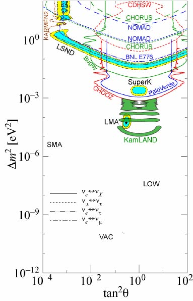
Figure 1: Summary of the currently allowed regions from a global analysis of atmospheric and solar neutrino experiments including first results from KamLAND (from H.Murayama’s web site http://hitoshi.berkeley.edu/neutrino/.)

In 1998 the Super-Kamiokande experiment published a paper [11] which represents a watershed in the history of neutrino physics. Super-Kamiokande measured the number of electron and muon neutrinos that arrive at the Earth’s surface as a result of cosmic ray interactions in the upper atmosphere, which are referred to as “atmospheric neutrinos”. While the number and and angular distribution of electron neutrinos is as expected, Super-Kamiokande showed that the number of muon neutrinos is significantly smaller than expected and that the flux of muon neutrinos exhibits a strong dependence on the zenith angle. These observations gave compelling evidence that muon neutrinos undergo flavour oscillations and this in turn implies that at least one neutrino flavour has a non-zero mass. The standard interpretation is that muon neutrinos are oscillating into tau neutrinos.

Current atmospheric neutrino oscillation data are well described by simple two-state mixing

$$\left(\begin{array}[]{c}\nu_{\mu}\\ \nu_{\tau}\end{array}\\ \right)=\left(\begin{array}[]{cc}\cos\theta_{23}&\sin\theta_{23}\\ -\sin\theta_{23}&\cos\theta_{23}\\ \end{array}\right)\left(\begin{array}[]{c}\nu_{2}\\ \nu_{3}\end{array}\\ \right)\;,$$ (1)

and the two-state Probability oscillation formula

$$P(\nu_{\mu}\rightarrow\nu_{\tau})=\sin^{2}2\theta_{23}\sin^{2}(1.27\Delta m_{32}^{2}{L}/{E})$$ (2)

where

$$\Delta m^{2}_{ij}\equiv m^{2}_{i}-m^{2}_{j}\;$$ (3)

and $m_{i}$ are the physical neutrino mass eigenvalues associated with the mass eigenstates $\nu_{i}$. $\Delta m_{32}^{2}$ is in units of eV², the baseline $L$ is in km and the beam energy $E$ is in GeV.

The atmospheric data is statistically dominated by the Super-Kamiokande results and the latest reported data sample as of the time of writing leads to:

$$\sin^{2}2\theta_{23}>0.92,\ \ 1.3\times 10^{-3}eV^{2}<|\Delta m_{32}^{2}|<3.0\times 10^{-3}eV^{2}(90\%CL)$$ (4)

The Super-Kamiokande region is shown in Fig.1. The atmospheric neutrino data is thus consistent with maximal $\nu_{\mu}-\nu_{\tau}$ neutrino mixing $\theta_{23}\approx\pi/4$ with $|\Delta m_{32}^{2}|\approx 2.5\times 10^{-3}{\rm eV}^{2}$ and the sign of $\Delta m_{32}^{2}$ undetermined. The maximal mixing angle means that we identify the heavy atmospheric neutrino of mass $m_{3}$ as being approximately

$$\nu_{3}\approx\frac{\nu_{\mu}+\nu_{\tau}}{\sqrt{2}}$$ (5)

and in addition there is a lighter orthogonal combination of mass $m_{2}$,

$$\nu_{2}\approx\frac{\nu_{\mu}-\nu_{\tau}}{\sqrt{2}}.$$ (6)

2.2 Three family solar neutrino mixing

Super-Kamiokande is also sensitive to the electron neutrinos arriving from the Sun, the “solar neutrinos”, and has independently confirmed the reported deficit of such solar neutrinos long reported by other experiments. For example Davis’s Homestake Chlorine experiment which began data taking in 1970 consists of 615 tons of tetrachloroethylene, and uses radiochemical techniques to determine the Ar37 production rate. More recently the SAGE and Gallex experiments contain large amounts of Ga71 which is converted to Ge71 by low energy electron neutrinos arising from the dominant pp reaction in the Sun. The combined data from these and other experiments implies an energy dependent suppression of solar neutrinos which can be interpreted as due to flavour oscillations. Taken together with the atmospheric data, this requires that a second neutrino flavour has a non-zero mass. The standard interpretation is that the electron neutrinos $\nu_{e}$ oscillate into the light linear combination $\nu_{2}\approx\frac{\nu_{\mu}-\nu_{\tau}}{\sqrt{2}}$.

SNO measurements of charged current (CC) reaction on deuterium is sensitive exclusively to $\nu_{e}$’s, while the elastic scattering (ES) off electrons also has a small sensitivity to $\nu_{\mu}$’s and $\nu_{\tau}$’s. The CC ratio is significantly smaller than the ES ratio. This immediately disfavours oscillations of $\nu_{e}^{\prime}s$ to sterile neutrinos which would lead to a diminished flux of electron neutrinos, but equal CC and ES ratios. On the other hand the different ratios are consistent with oscillations of $\nu_{e}$’s to active neutrinos $\nu_{\mu}$’s and $\nu_{\tau}$’s since this would lead to a larger ES rate since this has a neutral current component. The SNO analysis is nicely consistent with both the hypothesis that electron neutrinos from the Sun oscillate into other active flavours, and with the Standard Solar Model prediction. The latest results from SNO including the data taken with salt inserted into the detector to boost the efficiency of detecting the neutral current events [12], strongly favour the large mixing angle (LMA) MSW solution. In other words there is no longer any solar neutrino problem: we have instead solar neutrino mass!

The minimal neutrino sector required to account for the atmospheric and solar neutrino oscillation data thus consists of three light physical neutrinos with left-handed flavour eigenstates, $\nu_{e}$, $\nu_{\mu}$, and $\nu_{\tau}$, defined to be those states that share the same electroweak doublet as the left-handed charged lepton mass eigenstates. Within the framework of three–neutrino oscillations, the neutrino flavor eigenstates $\nu_{e}$, $\nu_{\mu}$, and $\nu_{\tau}$ are related to the neutrino mass eigenstates $\nu_{1}$, $\nu_{2}$, and $\nu_{3}$ with mass $m_{1}$, $m_{2}$, and $m_{3}$, respectively, by a $3\times 3$ unitary matrix called the lepton mixing matrix $U$ [13]

$$\left(\begin{array}[]{c}\nu_{e}\\ \nu_{\mu}\\ \nu_{\tau}\end{array}\\ \right)=\left(\begin{array}[]{ccc}U_{e1}&U_{e2}&U_{e3}\\ U_{\mu 1}&U_{\mu 2}&U_{\mu 3}\\ U_{\tau 1}&U_{\tau 2}&U_{\tau 3}\\ \end{array}\right)\left(\begin{array}[]{c}\nu_{1}\\ \nu_{2}\\ \nu_{3}\end{array}\\ \right)\;.$$ (7)

Assuming the light neutrinos are Majorana, $U$ can be parameterized in terms of three mixing angles $\theta_{ij}$ and three complex phases $\delta_{ij}$. A unitary matrix has six phases but three of them are removed by the phase symmetry of the charged lepton Dirac masses. Since the neutrino masses are Majorana there is no additional phase symmetry associated with them, unlike the case of quark mixing where a further two phases may be removed.

If we suppose to begin with that the phases are zero, then the lepton mixing matrix may be parametrised by a product of three Euler rotations,

$$U=R_{23}R_{13}R_{12}$$ (8)

where

$$R_{23}=\left(\begin{array}[]{ccc}1&0&0\\ 0&c_{23}&s_{23}\\ 0&-s_{23}&c_{23}\\ \end{array}\right)$$ (9)

$$R_{13}=\left(\begin{array}[]{ccc}c_{13}&0&s_{13}\\ 0&1&0\\ -s_{13}&0&c_{13}\\ \end{array}\right)$$ (10)

$$R_{12}=\left(\begin{array}[]{ccc}c_{12}&s_{12}&0\\ -s_{12}&c_{12}&0\\ 0&0&1\\ \end{array}\right)$$ (11)

where $c_{ij}=\cos\theta_{ij}$ and $s_{ij}=\sin\theta_{ij}$. Note that the allowed range of the angles is $0\leq\theta_{ij}\leq\pi/2$.

CHOOZ is a reactor experiment that falied to see any signal of neutrino oscillations over the Super-Kamiokande mass range. CHOOZ data from $\bar{\nu}_{e}\rightarrow\bar{\nu}_{e}$ disappearance not being observed provides a significant constraint on $\theta_{13}$ over the Super-Kamiokande (SK) prefered range of $\Delta m_{32}^{2}$ [14]:

$$\sin^{2}2\theta_{13}<0.1-0.3$$ (12)

The CHOOZ experiment therefore limits $\theta_{13}\stackrel{{\scriptstyle<}}{{{}_{\sim}}}0.2$ over the favoured atmospheric range, as shown in Fig.1.

KamLAND is a more powerful reactor experiment that measures $\bar{\nu}_{e}$’s produced by surrounding nuclear reactors. KamLAND has already seen a signal of neutrino oscillations over the LMA MSW mass range, and has recently confirmed the LMA MSW region “in the laboratory” [15]. KamLAND and SNO results when combined with other solar neutrino data especially that of Super-Kamiokande uniquely specify the large mixing angle (LMA) MSW [10] solar solution with three active light neutrino states, a large solar angle

$$\tan^{2}\theta_{12}\approx 0.4,\ \ \Delta m_{21}^{2}\approx 7\times 10^{-5}{\rm eV}^{2}.$$ (13)

according to the most recent global fits [16] performed after the SNO salt data [12]. KamLAND has thus not only confirmed solar neutrino oscillations, but have also uniquely specified the large mixing angle (LMA) solar solution, heralding a new era of precision neutrino physics.

The currently regions of atmospheric and solar parameter space allowed by all experiments are depicted in Figure 1. In Figure 1 the atmospheric and LMA MSW solar regions are clearly shown as elliptical regions, with the SMA, LOW and VAC regions now having disappeared. One of the KamLAND rate plus shape allowed regions shown in Figure 1 intersects the central part of the LMA ellipse near the best fit LMA point as determined from the solar data alone, thereby confirming the LMA MSM solution.

2.3 Summary of neutrino mixing angles and mass patterns

The current experimental situation is summarized by $\theta_{23}\approx\pi/4$, $\theta_{13}\leq 0.2$, and $\theta_{12}\approx\pi/6$. Ignoring phases, the relation between the neutrino flavor eigenstates $\nu_{e}$, $\nu_{\mu}$, and $\nu_{\tau}$ and the neutrino mass eigenstates $\nu_{1}$, $\nu_{2}$, and $\nu_{3}$ is just given as a product of three Euler rotations in Eq.8 as depicted in Fig.2.

Figure 2: The relation between the neutrino flavor eigenstates $\nu_{e}$, $\nu_{\mu}$, and $\nu_{\tau}$ and the neutrino mass eigenstates $\nu_{1}$, $\nu_{2}$, and $\nu_{3}$ in terms of the three mixing angles $\theta_{12}$, $\theta_{13}$, $\theta_{23}$. The atmospheric angle is $\theta_{23}\approx\pi/4$, the CHOOZ angle is $\theta_{13}\stackrel{{\scriptstyle<}}{{{}_{\sim}}}0.2$, and the solar angle is $\theta_{12}\approx\pi/6$.

This corresponds to the approximate form of mixing matrix

$$U\approx\left(\begin{array}[]{rrr}c_{12}&s_{12}&\theta_{13}\\ -\frac{s_{12}}{\sqrt{2}}&\frac{c_{12}}{\sqrt{2}}&\frac{1}{\sqrt{2}}\\ \frac{s_{12}}{\sqrt{2}}&-\frac{c_{12}}{\sqrt{2}}&\frac{1}{\sqrt{2}}\end{array}\right)$$ (14)

where $\theta_{12}\approx\pi/6$ corresponds to $s_{12}\approx\frac{1}{{2}}$, $c_{12}\approx\frac{\sqrt{3}}{{2}}$.

It is clear that neutrino oscillations, which only depend on $\Delta m_{ij}^{2}\equiv m_{i}^{2}-m_{j}^{2}$, give no information about the absolute value of the neutrino mass squared eigenvalues $m_{i}^{2}$, and there are basically two patterns of neutrino mass squared orderings consistent with the atmospheric and solar data as shown in Fig.3.

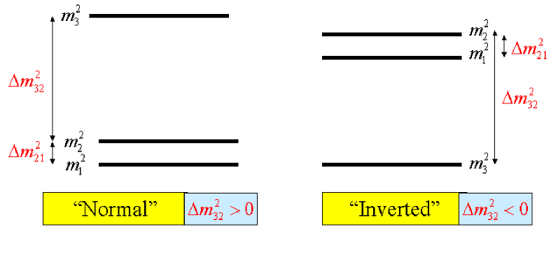
Figure 3: Alternative neutrino mass patterns that are consistent with neutrino oscillation explanations of the atmospheric and solar data. The absolute scale of neutrino masses is not fixed by oscillation data and the lightest neutrino mass may vary from 0.0-0.23 eV.

2.4 Three family neutrino mixing with phases

Including the phases, assuming the light neutrinos are Majorana, $U$ can be parameterized in terms of three mixing angles $\theta_{ij}$, a Dirac phase $\delta$, together with two Majorana phases $\beta_{1},\beta_{2}$, as follows

$$U=R_{23}U_{13}R_{12}P_{12}$$ (15)

where

$$U_{13} = \left(\begin{array}[]{ccc}c_{13}&0&s_{13}e^{-i\delta}\\ 0&1&0\\ -s_{13}e^{i\delta}&0&c_{13}\\ \end{array}\right),$$ (19)

$$P_{12} = \left(\begin{array}[]{ccc}e^{i\beta_{1}}&0&0\\ 0&e^{i\beta_{2}}&0\\ 0&0&1\\ \end{array}\right)$$ (23)

where $c_{ij}=\cos\theta_{ij}$ and $s_{ij}=\sin\theta_{ij}$, and $R_{23},R_{12}$ were defined below Eq.8.

Alternatively the lepton mixing matrix may be expressed as a product of three complex Euler rotations,

$$U=U_{23}U_{13}U_{12}$$ (24)

where

$$U_{23}=\left(\begin{array}[]{ccc}1&0&0\\ 0&c_{23}&s_{23}e^{-i\delta_{23}}\\ 0&-s_{23}e^{i\delta_{23}}&c_{23}\\ \end{array}\right)$$ (25)

$$U_{13}=\left(\begin{array}[]{ccc}c_{13}&0&s_{13}e^{-i\delta_{13}}\\ 0&1&0\\ -s_{13}e^{i\delta_{13}}&0&c_{13}\\ \end{array}\right)$$ (26)

$$U_{12}=\left(\begin{array}[]{ccc}c_{12}&s_{12}e^{-i\delta_{12}}&0\\ -s_{12}e^{i\delta_{12}}&c_{12}&0\\ 0&0&1\\ \end{array}\right)$$ (27)

The equivalence of different parametrisations of the lepton mixing matrix, and the relation between them is discussed in Appendix A.

Three family oscillation probabilities depend upon the time–of–flight (and hence the baseline $L$), the $\Delta m^{2}_{ij}$, and $U$ (and hence $\theta_{12},\theta_{23},\theta_{13}$, and $\delta$). Three-state neutrino mixing is discussed in Appendix B. Since we have assumed that the neutrinos are Majorana, there are two extra phases, but only one combination $\delta=\delta_{13}-\delta_{23}-\delta_{12}$ affects oscillations. If the neutrinos are Dirac, then the phases $\beta_{1}=\beta_{2}=0$, but the phase $\delta$ remains.

2.5 The LSND signal

The signal of another independent mass splitting from the LSND accelerator experiment [17] would either require a further light neutrino state with no weak interactions (a so-called “sterile neutrino”) or some other non-standard physics. This effect has not been confirmed by a similar experiment KARMEN [18], and currently a decisive experiment MiniBooNE is underway to decide the issue. In Figure 1 the LSND signal region is indicated, together with the KARMEN excluded region.

2.6 Future experimental prospects

Further experimental progress from SNO and KamLAND will consist of pinning down LMA MSW parameters to high accuracy. Neutrino physics has, now entered the precision era. Future neutrino oscillation experiments, will give accurate information about the mass squared splittings $\Delta m_{ij}^{2}\equiv m_{i}^{2}-m_{j}^{2}$, mixing angles, and CP violating phase. In the near future much better solar neutrino measurements will be available as KamLAND, SNO and Borexino furnish us with new and better data. The K2K long baseline (LBL) experiment from KEK to Super-Kamiokande has recently reported results in its phases I and II, which cover the atmospheric region and support the Super-Kamiokande results. In the longer term LBL experiments such as MINOS and eventually the CERN to Gran Sasso experiments will given more accurate determinations of the atmospheric parameters, eventually to 10%. J-PARC will be an “off-axis superbeam” over a LBL of 295 km to Super-Kamiokande due to start in 2008. Its first goal is to measure $\theta_{13}$ or set a limit on it of about 0.05 (as compared to the CHOOZ limit on $\theta_{13}$ of about 0.2). Interestingly MINOS over a LBL of 735 km is more sensitive than J-PARC to matter effects, so there should be some interesting complementarity between these two experiments, which could for example allow the sign of $\Delta m^{2}_{32}$ to be determined. The ultimate goal of oscillation experiments however is to measure the CP violating phase $\delta$. An upgraded J-PARC with a 4MW proton driver and a 1 megaton Hyper-Kamiokande detector, or some sort of Neutrino Factory based on muon storage rings would seem to be required for this purpose [19].

Oscillation experiments are not capable of telling us anything about the absolute scale of neutrino masses. The Tritium beta decay experiment KATRIN will tell us about the absolute scale of neutrino mass down to about 0.35 eV. The neutrinoless double beta decay experiment GENIUS will probe the Majorana nature of the electron neutrino down to about 0.01 eV [20]. Recent results from the 2dF galaxy redshift survey and WMAP, when combined with oscillation data, give the strong limit on the absolute mass of each neutrino species of about 0.23 eV [21, 22]. Turning to astrophysics, a galactic supernova could give valuable information about neutrino masses [23]. In future detection of energetic neutrinos from gamma ray bursts (GRBs), by neutrino telescopes such as ANTARES or ICECUBE could also provide important astrophysical information, and may provide another means of probing neutrino mass, and even quantum gravity [24].

2.7 Charged lepton contributions to neutrino masses and mixing angles

Although we refer to neutrino masses and mixing angles, it is worth pointing out that in general they could originate, at least in part, from the charged lepton sector. The (low energy) Lagrangian involving the charged lepton and neutrino mass matrices

$${\cal L}_{mass} =- (\bar{e}_{L1}\bar{e}_{L2}\bar{e}_{L3})m^{E}_{LR}({e}_{R1}{e}_{R2}{e}_{R3})^{T}$$ (28)

$$- \frac{1}{2}(\bar{\nu}_{L1}\bar{\nu}_{L2}\bar{\nu}_{L3})m_{LL}({\nu}_{L1}^{c}{\nu}_{L2}^{c}{\nu}_{L3}^{c})^{T}+H.c.$$

where $e_{Li}$ are the three left-handed charged lepton states, $e_{Ri}$ are the right-handed charged lepton states, $\nu_{Li}$ are the three left-handed neutrino states, and $\nu_{Li}^{c}$ are their CP conjugates. Note that the states $\nu_{Li}$ are not the mass eigenstate neutrinos since $m_{LL}$ is not diagonal in general. We shall refer to the mass eigenstate neutrinos as $\nu_{i}$ (without the L subscript), as in Eq.7.

In general the neutrino and charged lepton masses are given by the eigenvalues of a complex charged lepton mass matrix $m^{E}_{LR}$ and a complex symmetric neutrino Majorana matrix $m_{LL}$, obtained by diagonalising these mass matrices,

$$V^{E_{L}}m^{E}_{LR}{V^{E_{R}}}^{\dagger}=\left(\begin{array}[]{ccc}m_{e}&0&0\\ 0&m_{\mu}&0\\ 0&0&m_{\tau}\end{array}\right)$$ (29)

$$V^{\nu_{L}}m_{LL}{V^{\nu_{L}}}^{T}=\left(\begin{array}[]{ccc}m_{1}&0&0\\ 0&m_{2}&0\\ 0&0&m_{3}\end{array}\right)$$ (30)

where $V^{E_{L}}$, $V^{E_{R}}$, $V^{\nu_{L}}$ are unitary tranformations on the left-handed charged lepton fields $E_{L}$, right-handed charged lepton fields $E_{R}$, and left-handed neutrino fields $\nu_{L}$ which put the mass matrices into diagonal form with real eigenvalues.

After having diagonalised the mass matrices, the lepton mixing matrix is then constructed by

$$U=V^{E_{L}}{V^{\nu_{L}}}^{\dagger}$$ (31)

A unitary three dimensional matrix has six independent phases. As discussed in Appendix B, the freedom in the charged lepton phase enables three of the phases to be removed from $U$ to leave three phases. Since we have assumed that the neutrinos are Majorana, there is no further phase freedom, and the three remaining phases are physical (unlike the case of Dirac neutrinos where a further two phases can be removed, analagous to the case of the CKM matrix in the quark sector). Having constructed the lepton mixing matrix as discussed above, it may then be parametrised as discussed in section 2. Having done this one may then ask how much of a contribution to a particular mixing angle or phase, comes from the neutrino sector, and how much comes from the charged lepton sector. The lepton mixing matrix is constructed in Eq.23 as a product of a unitary matrix from the charged lepton sector $V^{E_{L}}$ and a unitary matrix from the neutrino sector ${V^{\nu_{L}}}^{\dagger}$. Each of these unitary matrices may be parametrised by its own mixing angles and phases analagous to the lepton mixing matrix parameters. As shown in Appendix C [26] the lepton mixing matrix can be expanded in terms of neutrino and charged lepton mixing angles and phases to leading order in the charged lepton mixing angles which are assumed to be small,

$$s_{23}e^{-i\delta_{23}} \approx s_{23}^{\nu_{L}}e^{-i\delta_{23}^{\nu_{L}}}-\theta_{23}^{E_{L}}c_{23}^{\nu_{L}}e^{-i\delta_{23}^{E_{L}}}$$ (32)

$$\theta_{13}e^{-i\delta_{13}} \approx \theta_{13}^{\nu_{L}}e^{-i\delta_{13}^{\nu_{L}}}-\theta_{13}^{E_{L}}c_{23}^{\nu_{L}}e^{-i\delta_{13}^{E_{L}}}$$ (33)

$$+ \theta_{12}^{E_{L}}s_{23}^{\nu_{L}}e^{i(-\delta_{23}^{\nu_{L}}-\delta_{12}^{E_{L}})}$$

$$s_{12}e^{-i\delta_{12}} \approx s_{12}^{\nu_{L}}e^{-i\delta_{12}^{\nu_{L}}}+\theta_{23}^{E_{L}}s_{12}^{\nu_{L}}e^{-i\delta_{12}^{\nu_{L}}}$$ (34)

$$+ \theta_{13}^{E_{L}}c_{12}^{\nu_{L}}s_{23}^{\nu_{L}}e^{i(\delta_{23}^{\nu_{L}}-\delta_{13}^{E_{L}})}$$

$$- \theta_{12}^{E_{L}}c_{23}^{\nu_{L}}c_{12}^{\nu_{L}}e^{-i\delta_{12}^{E_{L}}}$$

Clearly $\theta_{13}$ receives important contributions not just from $\theta_{13}^{\nu_{L}}$, but also from the charged lepton angles $\theta_{12}^{E_{L}}$, and $\theta_{13}^{E_{L}}$. In models where $\theta_{13}^{\nu_{L}}$ is extremely small, $\theta_{13}$ may originate almost entirely from the charged lepton sector. Charged lepton contributions could also be important in models where $\theta_{12}^{\nu_{L}}=\pi/4$, since charged lepton mixing angles may allow consistency with the LMA MSW solution. Such effects are important for the inverted hierarchy model [26].

Note that it is useful and possible to be able to diagonalise the mass matrices analytically, at least to first order in the small 13 mixing angles, but allowing the 23 and 12 angles to be large, while retaining all the phases. The proceedure for doing this is discussed for a hierarchical general mass matrix in Appendix D.1, for a hierarchical neutrino mass matrix in Appendix D.2, and for an inverted hierarchical neutrino mass matrix in Appendix D.3. The analytic results in these Appendices enable the separate mixing angles and phases associated with each of the unitary transformations $V^{E_{L}}$ and ${V^{\nu_{L}}}^{\dagger}$ to be obtained in many useful cases of interest.

2.8 The neutrino mass matrix

For many (but not all) purposes it is convenient to forget about the division between charged lepton and neutrino mixing angles and work in a basis where the charged lepton mass matrix is diagonal. Then the lepton mixing angles and phases simply correspond to the neutrino ones. In this special basis the mass matrix is given from Eq.30 and Eq.23 as

$$m_{LL}=U\left(\begin{array}[]{ccc}m_{1}&0&0\\ 0&m_{2}&0\\ 0&0&m_{3}\end{array}\right)U^{T}$$ (35)

For a given assumed form of $U$ and set of neutrino masses $m_{i}$ one may use Eq.35 to “derive” the form of the neutrino mass matrix $m_{LL}$, and this results in the candidate mass matrices in Table 1 [28]. Only the leading order forms are displayed explicitly in Table 1, and more accurate structures may be obtained case by case.

Table 1: Leading order low energy neutrino Majorana mass matrices $m_{LL}$ consistent with large atmospheric and solar mixing angles, classified according to the rate of neutrinoless double beta decay and the pattern of neutrino masses.

	Type I	Type II
	Small $\beta\beta_{0\nu}$	Large $\beta\beta_{0\nu}$
A	$\beta\beta_{0\nu}\stackrel{{\scriptstyle<}}{{{}_{\sim}}}0.0082$ eV
Normal hierarchy
$m_{1}^{2},m_{2}^{2}\ll m_{3}^{2}$	$\left(\begin{array}[]{ccc}0&0&0\\ 0&1&1\\ 0&1&1\\ \end{array}\right)\frac{m}{2}$	–
B	$\beta\beta_{0\nu}\stackrel{{\scriptstyle<}}{{{}_{\sim}}}0.0082$ eV	$\beta\beta_{0\nu}\stackrel{{\scriptstyle>}}{{{}_{\sim}}}0.0085$ eV
Inverted hierarchy
$m_{1}^{2}\approx m_{2}^{2}\gg m_{3}^{2}$	$\left(\begin{array}[]{ccc}0&1&1\\ 1&0&0\\ 1&0&0\\ \end{array}\right)\frac{m}{\sqrt{2}}$	$\left(\begin{array}[]{ccc}1&0&0\\ 0&\frac{1}{2}&\frac{1}{2}\\ 0&\frac{1}{2}&\frac{1}{2}\\ \end{array}\right)m$
C		$\beta\beta_{0\nu}\stackrel{{\scriptstyle>}}{{{}_{\sim}}}0.035$ eV
Approximate degeneracy		diag(1,1,1)m
$m_{1}^{2}\approx m_{2}^{2}\approx m_{3}^{2}$	$\left(\begin{array}[]{ccc}0&\frac{1}{\sqrt{2}}&\frac{1}{\sqrt{2}}\\ \frac{1}{\sqrt{2}}&\frac{1}{2}&\frac{1}{2}\\ \frac{1}{\sqrt{2}}&\frac{1}{2}&\frac{1}{2}\\ \end{array}\right)m$	$\left(\begin{array}[]{ccc}1&0&0\\ 0&0&1\\ 0&1&0\\ \end{array}\right)m$

In Table 1 the mass matrices are classified into two types:

Type I - small neutrinoless double beta decay

Type II - large neutrinoless double beta decay

They are also classified into the limiting cases consistent with the mass squared orderings in Fig.3:

A - Normal hierarchy $m_{1}^{2},m_{2}^{2}\ll m_{3}^{2}$

B - Inverted hierarchy $m_{1}^{2}\approx m_{2}^{2}\gg m_{3}^{2}$

C - Approximate degeneracy $m_{1}^{2}\approx m_{2}^{2}\approx m_{3}^{2}$

Thus according to our classification there is only one neutrino mass matrix consistent with the normal neutrino mass hierarchy which we call Type IA, corresponding to the leading order neutrino masses of the form $m_{i}=(0,0,m)$. For the inverted hierarchy there are two cases, Type IB corresponding to $m_{i}=(m,-m,0)$ or Type IIB corresponding to $m_{i}=(m,m,0)$. For the approximate degeneracy cases there are three cases, Type IC correponding to $m_{i}=(m,-m,m)$ and two examples of Type IIC corresponding to either $m_{i}=(m,m,m)$ or $m_{i}=(m,m,-m)$.

At present experiment allows any of the matrices in Table 1. In future it will be possible to uniquely specify the neutrino matrix in the following way:

1. Neutrinoless double beta effectively measures the 11 element of the mass matrix $m_{LL}$ corresponding to

$$\beta\beta_{0\nu}\equiv\sum_{i}U_{ei}^{2}m_{i}$$ (36)

and is clearly capable of resolving Type I from Type II cases according to the bounds given in Table 1 [29]. There has been a recent claim of a signal in neutrinoless double beta decay correponding to $\beta\beta_{0\nu}=0.11-0.56$ eV at 95% C.L. [30]. However this claim has been criticised by two groups [31], [32] and in turn this criticism has been refuted [33]. Since the Heidelberg-Moscow experiment has almost reached its full sensitivity, we may have to wait for a next generation experiment such as GENIUS [20] which is capable of pushing down the sensitivity to 0.01 eV to resolve this question.

2. A neutrino factory will measure the sign of $\Delta m_{32}^{2}$ and resolve A from B.

3. Tritium beta decay experiments are sensitive to C since they measure the “electron neutrino mass” defined by

$$|m_{\nu_{e}}|\equiv\sum_{i}|U_{ei}|^{2}|m_{i}|.$$ (37)

For example the KATRIN [34] experiment has a proposed sensitivity of 0.35 eV. As already mentioned the galaxy power spectrum combined with solar and atmospheric oscillation data already limits each neutrino mass to be less than about 0.23 eV, and this limit is also expected to improve in the future. Also it is worth mentioning that in future it may be possible to measure neutrino masses from gamma ray bursts using time of flight techniques in principle down to 0.001 eV [24].

Type IIB and C involve small fractional mass splittings $|\Delta m_{ij}^{2}|\ll m^{2}$ which are unstable under radiative corrections [35], and even the most natural Type IC case is difficult to implement [36],[37]. Types IA and IB seem to be the most natural cases.

Consider the case of full neutrino mass hierarchy $m_{3}\gg m_{2}\gg m_{1}\approx 0$, which is a special case of Type IA, where in this case $m_{3}\sim\sqrt{|\Delta m_{32}^{2}|}\sim 5.10^{-2}$ eV and $m_{2}\sim\sqrt{|\Delta m_{21}^{2}|}\sim 7.10^{-3}$ eV. From Eqs.14,35 we find the symmetric mass matrix,

$$m_{LL}\approx\left(\begin{array}[]{ccc}m_{2}s_{12}^{2}&\frac{1}{\sqrt{2}}(m_{2}s_{12}c_{12}+m_{3}\theta_{13})&-\frac{1}{\sqrt{2}}(m_{2}s_{12}c_{12}-m_{3}\theta_{13})\\ .&\frac{1}{{2}}(m_{3}+m_{2}c^{2}_{12})&\frac{1}{{2}}(m_{3}-m_{2}c^{2}_{12})\\ .&.&\frac{1}{{2}}(m_{3}+m_{2}c^{2}_{12})\end{array}\right)$$ (38)

neglecting terms like $m_{2}\theta_{13}$. Clearly this expression reduces to the leading Type IA form with $m=m_{3}$ in the approximation that $m_{2}$ and $\theta_{13}$ are neglected. However the more exact expression in Eq.38 shows that the required form of $m_{LL}$ should have a very definite detailed structure, which goes beyond the leading approximation in Table 1. For example the requirement $m_{2}\ll m_{3}$ implies that the sub-determinant of the mass matrix $m_{LL}$ is small:

$$det\left(\begin{array}[]{cc}m_{22}&m_{23}\\ m_{23}&m_{33}\\ \end{array}\right)\ll m_{3}^{2}.$$ (39)

This requirement in Eq.39 is satisfied by Eq.38, as may be readily seen, and this condition must be reproduced in a natural way (without fine-tuning) by any successful theory.

3 The See-Saw Mechanism

There are several different kinds of see-saw mechanism in the literature. In this review we shall focus on the simplest Type I see-saw mechanism, which we shall introduce below. However for completeness we shall also discuss the type II see-saw mechanism and the double see-saw mechanism.

3.1 Type I See-Saw

Before discussing the see-saw mechanism it is worth first reviewing the different types of neutrino mass that are possible. So far we have been assuming that neutrino masses are Majorana masses of the form

$$m_{LL}\overline{\nu_{L}}\nu_{L}^{c}$$ (40)

where $\nu_{L}$ is a left-handed neutrino field and $\nu_{L}^{c}$ is the CP conjugate of a left-handed neutrino field, in other words a right-handed antineutrino field. Such Majorana masses are possible to since both the neutrino and the antineutrino are electrically neutral and so Majorana masses are not forbidden by electric charge conservation. For this reason a Majorana mass for the electron would be strictly forbidden. However such Majorana neutrino masses violate lepton number conservation, and in the standard model, assuming only Higgs doublets are present, are forbidden at the renormalisable level by gauge invariance. The idea of the simplest version of the see-saw mechanism is to assume that such terms are zero to begin with, but are generated effectively, after right-handed neutrinos are introduced [5].

If we introduce right-handed neutrino fields then there are two sorts of additional neutrino mass terms that are possible. There are additional Majorana masses of the form

$$M_{RR}\overline{\nu_{R}}\nu_{R}^{c}$$ (41)

where $\nu_{R}$ is a right-handed neutrino field and $\nu_{R}^{c}$ is the CP conjugate of a right-handed neutrino field, in other words a left-handed antineutrino field. In addition there are Dirac masses of the form

$$m_{LR}\overline{\nu_{L}}\nu_{R}.$$ (42)

Such Dirac mass terms conserve lepton number, and are not forbidden by electric charge conservation even for the charged leptons and quarks.

Once this is done then the types of neutrino mass discussed in Eqs.41,42 (but not Eq.40 since we assume no Higgs triplets) are permitted, and we have the mass matrix

$$\left(\begin{array}[]{cc}\overline{\nu_{L}}&\overline{\nu^{c}_{R}}\end{array}\\ \right)\left(\begin{array}[]{cc}0&m_{LR}\\ m_{LR}^{T}&M_{RR}\\ \end{array}\right)\left(\begin{array}[]{c}\nu_{L}^{c}\\ \nu_{R}\end{array}\\ \right)$$ (43)

Since the right-handed neutrinos are electroweak singlets the Majorana masses of the right-handed neutrinos $M_{RR}$ may be orders of magnitude larger than the electroweak scale. In the approximation that $M_{RR}\gg m_{LR}$ the matrix in Eq.43 may be diagonalised to yield effective Majorana masses of the type in Eq.40,

$$m_{LL}=-m_{LR}M_{RR}^{-1}m_{LR}^{T}.$$ (44)

The effective left-handed Majorana masses $m_{LL}$ are naturally suppressed by the heavy scale $M_{RR}$. In a one family example if we take $m_{LR}=M_{W}$ and $M_{RR}=M_{GUT}$ then we find $m_{LL}\sim 10^{-3}$ eV which looks good for solar neutrinos. Atmospheric neutrino masses would require a right-handed neutrino with a mass below the GUT scale.

The see-saw mechanism can be formally derived from the following Lagrangian

$${\cal L}=-\bar{\nu}_{L}m_{LR}\nu_{R}-\frac{1}{2}\nu_{R}^{T}M_{RR}\nu_{R}+H.c.$$ (45)

where $\nu_{L}$ represents left-handed neutrino fields (arising from electroweak doublets), $\nu_{R}$ represents right-handed neutrino fields (arising from electroweak singlets), in a matrix notation where the $m_{LR}$ matrix elements are typically of order the charged lepton masses, while the $M_{RR}$ matrix elements may be much larger than the electroweak scale, and maybe up to the Planck scale. The number of right-handed neutrinos is not fixed, but the number of left-handed neutrinos is equal to three. Below the mass scale of the right-handed neutrinos we can integrate them out using the equations of motion

$$\frac{d{\cal L}}{\nu_{R}}=0$$ (46)

which gives

$$\nu_{R}^{T}=-\bar{\nu}_{L}m_{LR}M_{RR}^{-1},\ \ \nu_{R}=-M_{RR}^{-1}m_{LR}^{T}\bar{\nu}_{L}^{T}$$ (47)

Substituting back into the original Lagrangian we find

$${\cal L}=-\frac{1}{2}\bar{\nu}_{L}m_{LL}\nu_{L}^{c}+H.c$$ (48)

with $m_{LL}$ as in Eq.44.

3.2 Type II See-Saw and Double See-Saw

The version of the see-saw mechanism discussed so far is sometimes called the Type I see-saw mechanism. It is the simplest version of the see-saw mechanism, and can be thought of as resulting from integrating out heavy right-handed neutrinos to produce the effective dimension 5 neutrino mass operator

$$-\frac{1}{2}H_{u}L^{T}\kappa H_{u}L$$ (49)

where

$$\kappa=Y^{\nu}_{LR}M_{RR}^{-1}{Y^{\nu}_{LR}}^{T}.$$ (50)

One might wonder if it is possible to simply write down an operator by hand similar to Eq.49, without worrying about its origin. In fact, historically, such an operator was introduced suppressed by the Planck scale (rather than the right-handed neutrino mass scales) by Weinberg in order to account for small neutrino masses [38]. The problem is that such a Planck scale suppressed operator would lead to neutrino masses of order $10^{-5}{\rm eV}$ which are too small to account for $m_{2}$ or $m_{3}$ (though they could account for $m_{1}$). To account for $m_{3}$ requires dimension 5 operators suppressed by a mass scale of order $3\times 10^{14}$ GeV if the dimensionless coupling of the operator is of order unity, and the Higgs vev is equal to that of the Standard Model.

One might also wonder if the see-saw mechanism with right-handed neutrinos is the only possibility? In fact it is possible to generate the dimension 5 operator in Eq.49 by the exchange of heavy Higgs triplets of $SU(2)_{L}$, referred to as the type II see=saw mechanism.

Alternatively the see-saw can be implemented in a two-stage process by introducing additional neutrino singlets beyond the three right-handed neutrinos that we have considered so far. It is useful to distingush between “right-handed neutrinos” $\nu_{R}$ which carry $B-L$ and perhaps form $SU(2)_{R}$ doublets with right-handed charged leptons, and “neutrino singlets” $S$ which have no Yukawa couplings to the left-handed neutrinos, but which may couple to $\nu_{R}$. If the singlets have Majorana masses $M_{SS}$, but the right-handed neutrinos have a zero Majorana mass $M_{RR}=0$, the see-saw mechanism may proceed via mass couplings of singlets to right-handed neutrinos $M_{SR}$. In the basis $(\nu_{L},\nu_{R},S)$ the mass matrix is

$$\left(\begin{array}[]{ccc}0&m_{LR}&0\\ m_{LR}&0&M_{RS}\\ 0&M_{RS}^{T}&M_{SS}\end{array}\right)$$ (51)

Assuming $M_{SS}\ll M_{RS}$ the light physical left-handed Majorana neutrino masses are then doubly suppressed,

$$m_{LL}=m_{LR}M_{RS}^{-1}M_{SS}{M_{RS}^{T}}^{-1}m_{LR}^{T}$$ (52)

This is called the double see-saw mechanism. It is often used in string inspired neutrino mass models [39].

4 Right-Handed Neutrino Dominance

In this section we discuss an elegant and natural way of accounting for a neutrino mass hierarchy and two large mixing angles, by simply assuming that not all of the right-handed neutrinos contribute equally to physical neutrino masses in the see-saw mechanism. This mechanism, called sequential dominance, is a technique rather than a model, and can be applied to large classes of models. Indeed the conditions for sequential dominance can only be understood within particular models, and provide useful clues to the nature of such models.

4.1 Single Right-Handed Neutrino Dominance

With three left-handed neutrinos and three right-handed neutrinos the Dirac masses $m_{LR}$ are a $3\times 3$ (complex) matrix and the heavy Majorana masses $M_{RR}$ form a separate $3\times 3$ (complex symmetric) matrix. The light effective Majorana masses $m_{LL}$ are also a $3\times 3$ (complex symmetric) matrix and continue to be given from Eq.44 which is now interpreted as a matrix product. From a model building perspective the fundamental parameters which must be input into the see-saw mechanism are the Dirac mass matrix $m_{LR}$ and the heavy right-handed neutrino Majorana mass matrix $M_{RR}$. The light effective left-handed Majorana mass matrix $m_{LL}$ arises as an output according to the see-saw formula in Eq.44. The goal of see-saw model building is therefore to choose input see-saw matrices $m_{LR}$ and $M_{RR}$ that will give rise to one of the successful matrices $m_{LL}$ in Table 1.

We now show how the input see-saw matrices can be simply chosen to give the Type IA matrix, with the property of a naturally small sub-determinant in Eq.39 using a mechanism first suggested in [40]. The idea was developed in [42] where it was called single right-handed neutrino dominance (SRHND) . SRHND was first successfully applied to the LMA MSW solution in [43].

To understand the basic idea of dominance, it is instructive to begin by discussing a simple $2\times 2$ example, where we have in mind applying this to the atmospheric mixing in the 23 sector:

$$M_{RR}=\left(\begin{array}[]{cc}Y&0\\ 0&X\end{array}\right),\ \ \ \ m_{LR}=\left(\begin{array}[]{cc}e&b\\ f&c\end{array}\right)$$ (53)

The see-saw formula in Eq.44 $m_{LL}=m_{LR}M_{RR}^{-1}m_{LR}^{T}$ gives:

$$m_{LL}=\left(\begin{array}[]{cc}\frac{e^{2}}{Y}+\frac{b^{2}}{X}&\frac{ef}{Y}+\frac{bc}{X}\\ \frac{ef}{Y}+\frac{bc}{X}&\frac{f^{2}}{Y}+\frac{c^{2}}{X}\end{array}\right)\approx\left(\begin{array}[]{cc}\frac{e^{2}}{Y}&\frac{ef}{Y}\\ \frac{ef}{Y}&\frac{f^{2}}{Y}\end{array}\right)$$ (54)

where the approximation in Eq.54 assumes that the right-handed neutrino of mass $Y$ is sufficiently light that it dominates in the see-saw mechanism:

$$\frac{e^{2},f^{2},ef}{Y}\gg\frac{b^{2},c^{2},bc}{X}.$$ (55)

The neutrino mass spectrum from Eq.54 then consists of one neutrino with mass $m_{3}\approx(e^{2}+f^{2})/Y$ and one naturally light neutrino $m_{2}\ll m_{3}$, since the determinant of Eq.54 is clearly approximately vanishing, due to the dominance assumption [40]. The atmospheric angle from Eq.54 is $\tan\theta_{23}\approx e/f$ [40] which can be large or maximal providing $e\approx f$, even in the case $e,f,b\ll c$ that the neutrino Dirac mixing angles arising from Eq.53 are small. Thus two crucial features, namely a neutrino mass hierarchy $m_{3}^{2}\gg m_{2}^{2}$ and a large neutrino mixing angle $\tan\theta_{23}\approx 1$, can arise naturally from the see-saw mechanism assuming the dominance of a single right-handed neutrino. It was also realised that small perturbations from the sub-dominant right-handed neutrinos can then lead to a small solar neutrino mass splitting [40], as we now discuss.

4.2 Sequential Right-Handed Neutrino Dominance

In order to account for the solar and other mixing angles, we must generalise the above discussion to the $3\times 3$ case. The SRHND mechanism is most simply described assuming three right-handed neutrinos in the basis where the right-handed neutrino mass matrix is diagonal although it can also be developed in other bases [42, 43]. In this basis we write the input see-saw matrices as

$$M_{RR}=\left(\begin{array}[]{ccc}Y&0&0\\ 0&X&0\\ 0&0&X^{\prime}\end{array}\right)$$ (56)

$$m_{LR}=\left(\begin{array}[]{ccc}d&a&a^{\prime}\\ e&b&b^{\prime}\\ f&c&c^{\prime}\end{array}\right)$$ (57)

In [40] it was suggested that one of the right-handed neutrinos may dominante the contribution to $m_{LL}$ if it is lighter than the other right-handed neutrinos. The dominance condition was subsequently generalised to include other cases where the right-handed neutrino may be heavier than the other right-handed neutrinos but dominates due to its larger Dirac mass couplings [42]. In any case the dominant right-handed neutrino may be taken to be the one with mass $Y$ without loss of generality.

It was subsequently shown how to account for the LMA MSW solution with a large solar angle [43] by careful consideration of the sub-dominant contributions. One of the examples considered in [43] is when the right-handed neutrinos dominate sequentially,

$$\frac{|e^{2}|,|f^{2}|,|ef|}{Y}\gg\frac{|xy|}{X}\gg\frac{|x^{\prime}y^{\prime}|}{X^{\prime}}$$ (58)

which is the straightforward generalisation of Eq.55 where $x,y\in a,b,c$ and $x^{\prime},y^{\prime}\in a^{\prime},b^{\prime},c^{\prime}$. Assuming SRHND with sequential sub-dominance as in Eq.58, then Eqs.44, 56, 57 give

$$m_{LL}\approx\left(\begin{array}[]{ccc}\frac{a^{2}}{X}+\frac{d^{2}}{Y}&\frac{ab}{X}+\frac{de}{Y}&\frac{ac}{X}+\frac{df}{Y}\\ .&\frac{b^{2}}{X}+\frac{e^{2}}{Y}&\frac{bc}{X}+\frac{ef}{Y}\\ .&.&\frac{c^{2}}{X}+\frac{f^{2}}{Y}\end{array}\right)$$ (59)

where the contribution from the right-handed neutrino of mass $X^{\prime}$ may be neglected according to Eq.58. If the couplings satisfy the sequential dominance condition in Eq.58 then the matrix in Eq.59 resembles the Type IA matrix, and furthermore has a naturally small sub-determinant as in Eq.39. This leads to a full neutrino mass hierarchy

$$m_{3}^{2}\gg m_{2}^{2}\gg m_{1}^{2}$$ (60)

and, ignoring phases, the solar angle only depends on the sub-dominant couplings and is given by $\tan\theta_{12}\approx a/(c_{23}b-s_{23}c)$ [43]. The simple requirement for large solar angle is then $a\sim b-c$ [43].

Including phases the neutrino masses are given to leading order in $m_{2}/m_{3}$ by diagonalising the mass matrix in Eq.59 using the analytic proceedure described in Appendix D [26]. In the case that $d=0$, corresponding to a 11 texture zero in Eq.57, we have

$$m_{1} \sim O(\frac{x^{\prime}y^{\prime}}{X^{\prime}})$$ (61)

$$m_{2} \approx \frac{|a|^{2}}{Xs_{12}^{2}}$$ (62)

$$m_{3} \approx \frac{|e|^{2}+|f|^{2}}{Y}$$ (63)

where $s_{12}=\sin\theta_{12}$ is given below. Note that with SD each neutrino mass is generated by a separate right-handed neutrino, and the sequential dominance condition naturally results in a neutrino mass hierarchy $m_{1}\ll m_{2}\ll m_{3}$. The neutrino mixing angles are given to leading order in $m_{2}/m_{3}$ by,

$$\tan\theta_{23} \approx \frac{|e|}{|f|}$$ (64)

$$\tan\theta_{12} \approx \frac{|a|}{c_{23}|b|\cos(\tilde{\phi}_{b})-s_{23}|c|\cos(\tilde{\phi}_{c})}$$ (65)

$$\theta_{13} \approx e^{i(\tilde{\phi}+\phi_{a}-\phi_{e})}\frac{|a|(e^{*}b+f^{*}c)}{[|e|^{2}+|f|^{2}]^{3/2}}\frac{Y}{X}$$ (66)

where we have written some (but not all) complex Yukawa couplings as $x=|x|e^{i\phi_{x}}$. The phase $\delta$ is fixed to give a real angle $\theta_{12}$ by,

$$c_{23}|b|\sin(\tilde{\phi}_{b})\approx s_{23}|c|\sin(\tilde{\phi}_{c})$$ (67)

where

$$\tilde{\phi}_{b} \equiv \phi_{b}-\phi_{a}-\tilde{\phi}+\delta,$$

$$\tilde{\phi}_{c} \equiv \phi_{c}-\phi_{a}+\phi_{e}-\phi_{f}-\tilde{\phi}+\delta$$ (68)

The phase $\tilde{\phi}$ is fixed to give a real angle $\theta_{13}$ by,

$$\tilde{\phi}\approx\phi_{e}-\phi_{a}-\phi_{\rm COSMO}$$ (69)

where

$$\phi_{\rm COSMO}=\arg(e^{*}b+f^{*}c).$$ (70)

is the leptogenesis phase [25] corresponding to the interference diagram involving the lightest and next-to-lightest right-handed neutrinos [26].

4.3 Types of Sequential Dominance

Assuming sequential dominance, there is still an ambiguity regarding the mass ordering of the heavy Majorana right-handed neutrinos. So far we have assumed that the dominant right-handed neutrino of mass $Y$ is dominant because it is the lightest one. We emphasise that this need not be the case. The neutrino of mass $Y$ could be dominant even if it is the heaviest right-handed neutrino, providing its Yukawa couplings are strong enough to overcome its heaviness and satisfy the condition in Eq.58. In hierarchical mass matrix models, it is natural to order the right-handed neutrinos so that the heaviest right-handed neutrino is the third one, the intermediate right-handed neutrino is the second one, and the lightest right-handed neutrino is the first one. It is also natural to assume that the 33 Yukawa coupling is of order unity, due to the large top quark mass. It is therefore possible that the dominant right-handed neutrino is the heaviest (called heavy sequential dominance or HSD), the lightest (called light sequential dominance or LSD), or the intermediate one (called intermediate sequential dominance or ISD). This leads to the six possible types of sequential dominance corresponding to the six possible mass orderings of the right-handed neutrinos as shown in Table1. In each case the dominant right-handed neutrino is the one with mass $Y$, and the leading subdominant right-handed neutrino is the one with mass $X$. The resulting see-saw matrix $m_{LL}$ is invariant under re-orderings of the right-handed neutrino columns, but the leading order form of the neutrino Yukawa matrix $Y_{\nu}$ is not.

Table 2: Types of sequential dominance (SD), classified according to the mass ordering of the right-handed neutrinos. Light sequential dominance (LSD) corresponds to the dominant right-handed neutrino of mass $Y$ being the lightest. Intermediate sequential dominance (ISD) corresponds to the dominant right-handed neutrino of mass $Y$ being the intermediate one. Heavy sequential dominance (HSD) corresponds to the dominant right-handed neutrino of mass $Y$ being the heaviest.

Type of SD	$M_{RR}$	$Y_{\nu}$	Leading $Y_{\nu}$
$\stackrel{{\scriptstyle\rm LSDa}}{{Y<X<X^{\prime}}}$	$\left(\begin{array}[]{ccc}Y&0&0\\ 0&X&0\\ 0&0&X^{\prime}\\ \end{array}\right)$	$\left(\begin{array}[]{ccc}d&a&a^{\prime}\\ e&b&b^{\prime}\\ f&c&c^{\prime}\\ \end{array}\right)$	$\left(\begin{array}[]{ccc}0&0&0\\ 0&0&0\\ 0&0&1\\ \end{array}\right)$
$\stackrel{{\scriptstyle\rm LSDb}}{{Y<X^{\prime}<X}}$	$\left(\begin{array}[]{ccc}Y&0&0\\ 0&X^{\prime}&0\\ 0&0&X\\ \end{array}\right)$	$\left(\begin{array}[]{ccc}d&a^{\prime}&a\\ e&b^{\prime}&b\\ f&c^{\prime}&c\\ \end{array}\right)$	$\left(\begin{array}[]{ccc}0&0&1\\ 0&0&1\\ 0&0&1\\ \end{array}\right)$
$\stackrel{{\scriptstyle\rm ISDa}}{{X<Y<X^{\prime}}}$	$\left(\begin{array}[]{ccc}X&0&0\\ 0&Y&0\\ 0&0&X^{\prime}\\ \end{array}\right)$	$\left(\begin{array}[]{ccc}a&d&a^{\prime}\\ b&e&b^{\prime}\\ c&f&c^{\prime}\\ \end{array}\right)$	$\left(\begin{array}[]{ccc}0&0&0\\ 0&0&0\\ 0&0&1\\ \end{array}\right)$
$\stackrel{{\scriptstyle\rm ISDb}}{{X^{\prime}<Y<X}}$	$\left(\begin{array}[]{ccc}X^{\prime}&0&0\\ 0&Y&0\\ 0&0&X\\ \end{array}\right)$	$\left(\begin{array}[]{ccc}a^{\prime}&d&a\\ b^{\prime}&e&b\\ c^{\prime}&f&c\\ \end{array}\right)$	$\left(\begin{array}[]{ccc}0&0&1\\ 0&0&1\\ 0&0&1\\ \end{array}\right)$
$\stackrel{{\scriptstyle\rm HSDa}}{{X^{\prime}<X<Y}}$	$\left(\begin{array}[]{ccc}X^{\prime}&0&0\\ 0&X&0\\ 0&0&Y\\ \end{array}\right)$	$\left(\begin{array}[]{ccc}a^{\prime}&a&d\\ b^{\prime}&b&e\\ c^{\prime}&c&f\\ \end{array}\right)$	$\left(\begin{array}[]{ccc}0&0&0\\ 0&0&1\\ 0&0&1\\ \end{array}\right)$
$\stackrel{{\scriptstyle\rm HSDb}}{{X<X^{\prime}<Y}}$	$\left(\begin{array}[]{ccc}X&0&0\\ 0&X^{\prime}&0\\ 0&0&Y\\ \end{array}\right)$	$\left(\begin{array}[]{ccc}a&a^{\prime}&d\\ b&b^{\prime}&e\\ c&c^{\prime}&f\\ \end{array}\right)$	$\left(\begin{array}[]{ccc}0&0&0\\ 0&0&1\\ 0&0&1\\ \end{array}\right)$

It is worth emphasising that since all the forms above give the same light effective see-saw neutrino matrix $m_{LL}$ in Eq.59, under the sequential dominance assumption in Eq.58, this implies that the analytic results for neutrino masses and mixing angles applies to all of these forms. They are distinguished theoretically by different preferred leading order forms of the neutrino Yukawa matrix $Y_{\nu}$ shown in the table. These leading order forms follow from the the large mixing angle requirements $e\sim f$ and $a\sim b-c$. Thus we see that LSDa, and ISDa are consistent with a form of Yukawa matrix with small Dirac mixing angles, while HSDa and HSDb correspond to the so called “lop-sided” forms. LSDb and ISDb correspond to the D-brane inspired “single right-handed democracy” form studied in [44]. They are also distinguished by leptogenesis and lepton flavour violation as we shall see.

For example, suppose that we impose the theoretical requirement that the neutrino Yukawa matrix resembles hierarchical quark matrices, and have a large 33 element of order unity, but no other large off-diagonal entries. Then the large mixing angle requirements $e\sim f$ and $a\sim b-c$ immediately excludes HSDa, HSDb, LSDb and ISDb. We are left with LSDa and ISDa as the remaining possibilities. If we further impose the requirement of a 11 texture zero, as motivated by the GST relation [45], then $a\sim b-c$ excludes ISDa, and we are left uniquely with LSDa. We shall later discuss an example of a realistic model of all quark and lepton masses and mixing angles based on LSDa. For now we note that that for LSDa in order to satisfy the sequential dominance condition in Eq.58 the heavy Majorana masses must be necessarily strongly hierarchical,

$$Y\ll X\ll X^{\prime}.$$ (71)

The reason is that the heavy right-handed neutrino of mass $X^{\prime}$ has order unity Yukawa couplings to left-handed neutrinos, which implies that the lightest right-handed neutrino of mass $Y$ must be significantly lighter in order to dominate.

4.4 Leptogenesis Link

It is interesting to note that in LSDa, assuming a 11 texture zero, there is a link between the CP violation required for leptogenesis, and the phase $\delta$ measurable in accurate neutrino oscillation experiments. This can be seen from Eq.70 which may be expressed as

$$\tan\phi_{\rm COSMO}\approx\frac{|b|s_{23}s_{2}+|c|c_{23}s_{3}}{|b|s_{23}c_{2}+|c|c_{23}c_{3}}.$$ (72)

From Eqs.69,67,68,

$$\tan(\phi_{\rm COSMO}+\delta)\approx\frac{|b|c_{23}s_{2}-|c|s_{23}s_{3}}{-|b|c_{23}c_{2}+|c|s_{23}c_{3}}$$ (73)

where we have written $s_{i}=\sin\eta_{i},c_{i}=\cos\eta_{i}$ where

$$\eta_{2}\equiv\phi_{b}-\phi_{e},\ \ \eta_{3}\equiv\phi_{c}-\phi_{f}$$ (74)

are invariant under a charged lepton phase transformation. The reason that the see-saw parameters only involve two invariant phases $\eta_{2},\eta_{3}$ rather than the usual six is due to the LSD assumption which has the effect of decoupling the heaviest right-handed neutrino, which removes three phases, together with the assumption of a 11 texture zero, which removes another phase.

Eq.73 shows that $\delta$ is a function of the two see-saw phases $\eta_{2},\eta_{3}$ that also determine $\phi_{\rm COSMO}$ in Eq.72. If both the phases $\eta_{2},\eta_{3}$ are zero, then both $\phi_{\rm COSMO}$ and $\delta$ are necessarily zero. This feature is absolutely crucial. It means that, barring cancellations, measurement of a non-zero value for the phase $\delta$ at a neutrino factory will be a signal of a non-zero value of the leptogenesis phase $\phi_{\rm COSMO}$. We also find the remarkable result

$$|\phi_{\rm COSMO}|=|\phi_{\beta\beta 0\nu}|.$$ (75)

where $\phi_{\beta\beta 0\nu}$ is the phase which enters the rate for neutrinoless double beta decay [46].

4.5 Comparison to the Smirnov Approach

An early approach to obtaining large mixing angles from the see-saw mechanism was proposed by [47], which is sometimes confused with sequential dominance. The purpose of this subsection is to briefly review the Smirnov approach, and explain how it differs from sequential dominance. The Smirnov approach for obtaining large mixing angles from the see-saw mechanism, is based on the theoretical assumption of having no large mixing angles in the Yukawa sector [47].

We shall briefly discuss the two family case considered in [47]. For this case the physical lepton mixing angle is written as

$$\theta\equiv\theta_{L}^{e_{LR}}-\theta_{L}^{\nu_{LR}}+\theta_{SS}$$ (76)

where $\theta_{L}^{e_{LR}}$ is the left-handed mixing angle which diagonalises the charge lepton Yukawa matrix, $\theta_{L}^{\nu_{LR}}$ is the left-handed mixing angle which diagonalises the neutrino Yukawa matrix, and $\theta_{SS}$ is defined to be the additional angle which results from the presence of the see-saw mechanism. The basic idea [47] was that a large mixing angle $\theta$ could originate from the see-saw mechanism via $\theta_{SS}$ with $\theta_{L}^{e_{LR}}$ and $\theta_{L}^{\nu_{LR}}$ being small. Smirnov obtains an approximate analytic expression for $\theta_{SS}$ in the two family case,

$$\tan\theta_{SS}\approx-2\epsilon^{D}\frac{\tan(\theta_{R}^{\nu_{LR}}-\theta_{R}^{\nu_{RR}})}{\tan^{2}(\theta_{R}^{\nu_{LR}}-\theta_{R}^{\nu_{RR}})+\epsilon^{M}}$$ (77)

where $\theta_{R}^{\nu_{LR}}$ is the mixing angle which diagonalises the neutrino Yukawa $Y^{\nu}_{LR}$ matrix on the right, $\theta_{R}^{\nu_{RR}}$ is the mixing angle which diagonalises the heavy Majorana neutrino matrix $M_{RR}$, $\epsilon^{D}$ is the ratio of neutrino Yukawa (Dirac) matrix eigenvalues, and $\epsilon^{M}$ is the ratio of heavy Majorana matrix eigenvalues. The conditions that $\theta_{SS}$ is large are

$$\tan(\theta_{R}^{\nu_{LR}}-\theta_{R}^{\nu_{RR}}) \leq \epsilon^{D}$$ (78)

$$\epsilon^{M} \leq (\epsilon^{D})^{2}$$ (79)

which, for a typical quark-like hierarchy $\epsilon^{D}\ll 1$, implies both a very accurate equality of mixing angles $\theta_{R}^{\nu_{LR}}=\theta_{R}^{\nu_{RR}}$ and very strongly hierarchical heavy Majorana masses (much stronger than the Dirac mass hierarchy).

The conditions in Eqs.78,79 are clearly nothing to do with sequential dominance in general. For one thing since some versions of sequential dominance involve large neutrino Yukawa mixing angles $\theta_{L}^{\nu_{LR}}$ and do not require $\theta_{SS}$ to be large, which is the basic assumption of this approach. However there are classes of sequential dominance model such as LSDa where $\theta_{L}^{\nu_{LR}}$ is small and $\theta_{SS}$ is large. Furthermore in this class of model there is a strong hierarchy of Majorana masses. One might be tempted to think that LSDa is the same as the Smirnov approach, and this has led to some confusion in the literature which we would like to clear up here. The important point to emphasise is that [47] never talks about one of the right-handed neutrinos giving the dominant contribution to the heaviest physical neutrino via the see-saw mechanism, or indeed about the relative contribution of the right-handed neutrinos to the see-saw mechanism in general. Thus there is no natural mechanism present for generating a neutrino mass hierarchy in [47], which is concerned only with the condition for generating large mixing angles. The point about sequential dominance is that it can naturally generate a neutrino mass hierarchy and large mixing angles, as simple ratios of Yukawa couplings of dominant and subdominant right-handed neutrinos.

A simple counter example will illustrate this point. Condider the following matrices,

$$M_{RR}=\left(\begin{array}[]{cc}A_{11}\epsilon_{D}^{2}&A_{12}\epsilon_{D}\\ A_{12}\epsilon_{D}&A_{22}\end{array}\right)M,\ \ {Y_{\nu}}_{LR}=\left(\begin{array}[]{ccc}a_{11}\epsilon_{D}&a_{12}\epsilon_{D}\\ a_{21}\epsilon_{D}&a_{22}\end{array}\right)$$ (80)

where $A_{ij},a_{ij}$ are order unity coefficients. These matrices clearly satisfy the conditions in Eqs.78,79, since $\theta_{R}^{\nu_{LR}}\sim\theta_{R}^{\nu_{RR}}\sim\epsilon_{D}$ and $\epsilon_{M}\sim\epsilon_{D}^{2}$. However these matrices do not satisfy the dominance conditions. Both right-handed neutrinos will contribute equally at $O(1/M)$ via the see-saw mechanism to the heaviest physical neutrino mass. Without the dominance of a single right-handed neutrino the neutrino mass hierarchy will require some tuning. The tuning required for the atmospheric mixing angle involving second and third families with be rather mild since $m_{2}/m_{3}$ is not so small, however when this scheme is extended to all three families, further tuning will be required to obtain a large solar mixing angle in a natural way. In actual examples given in [47] even more tuning is likely to be required since the angles $\theta_{R}^{\nu_{LR}},\theta_{R}^{\nu_{RR}}$ were both independently supposed to be larger than $\epsilon^{D}$.

The conclusion is that Smirnov’s approach did not recognise right-handed neutrino dominance, contrary to some recent claims in the literature, but it does provide a complementary approach to a large mixing angles from the see-saw mechanism. At first sight it appears to have some similarities to LSDa, however without the missing ingredient of sequential dominance, to achieve two large mixing angles together with a neutrino mass hierarchy will require some degree of fine-tuning. The conditions proposed by Smirnov are therefore neither necessary nor sufficient for right-handed neutrino dominance.

5 See-Saw Standard Models

In this section we show how the see-saw mechanism can be accomodated in the Standard Model and its Supersymmetric Extension, where it leads to lepton flavour violation.

5.1 Minimal See-Saw Standard Model

We now briefly discuss what the standard model looks like, assuming a minimal see-saw extension. In the standard model Dirac mass terms for charged leptons and quarks are generated from Yukawa couplings to Higgs doublets whose vacuum expectation value gives the Dirac mass term. Neutrino masses are zero in the Standard Model because right-handed neutrinos are not present, and also because the Majorana mass terms in Eq.40 require Higgs triplets in order to be generated at the renormalisable level. The simplest way to generate neutrino masses from a renormalisable theory is to introduce right-handed neutrinos, as in the Type I see-saw mechanism, which we assume here. The Lagrangian for the lepton sector of the standard model containing three right-handed neutrinos with heavy Majorana masses is

$${\cal L}_{mass}=-\epsilon_{ab}\left[\tilde{Y}^{e}_{ij}H_{d}^{a}L_{i}^{b}e^{c}_{j}-\tilde{Y}^{\nu}_{ij}H_{u}^{a}L_{i}^{b}\nu^{c}_{j}+\frac{1}{2}\nu^{c}_{i}\tilde{M}_{RR}^{ij}\nu^{c}_{j}\right]+H.c.$$ (81)

where $\epsilon_{ab}=-\epsilon_{ba}$, $\epsilon_{12}=1$, and the remaining notation is standard except that the $3$ right-handed neutrinos $\nu_{R}^{p}$ have been replaced by their CP conjugates $\nu^{c}_{i}$, and $\tilde{M}_{RR}^{ij}$ is a complex symmetric Majorana matrix. When the two Higgs doublets get their VEVS $<H_{u}^{2}>=v_{2}$, $<H_{d}^{1}>=v_{1}$, where the ratio of VEVs is defined to be $\tan\beta\equiv v_{2}/v_{1}$, we find the terms

$${\cal L}_{mass}=-v_{1}\tilde{Y}^{e}_{ij}e_{i}e^{c}_{j}-v_{2}\tilde{Y}^{\nu}_{ij}\nu_{i}\nu^{c}_{j}-\frac{1}{2}\tilde{M}_{RR}^{ij}\nu^{c}_{i}\nu^{c}_{j}+H.c.$$ (82)

Replacing CP conjugate fields we can write in a matrix notation

$${\cal L}_{mass}=-\bar{e}_{L}v_{1}\tilde{Y^{e}}^{\ast}e_{R}-\bar{\nu}_{L}v_{2}\tilde{Y^{\nu}}^{\ast}\nu_{R}-\frac{1}{2}\nu^{T}_{R}\tilde{M}_{RR}^{\ast}\nu_{R}+H.c.$$ (83)

It is convenient to work in the diagonal charged lepton basis

$${\rm diag(m_{e},m_{\mu},m_{\tau})}=V_{E_{L}}v_{1}\tilde{Y^{e}}^{\ast}V_{E_{R}}^{{\dagger}}$$ (84)

and the diagonal right-handed neutrino basis

$${\rm diag(M_{1},M_{2},M_{3})}=V_{\nu_{R}}\tilde{M^{\ast}}_{RR}V_{\nu_{R}}^{T}$$ (85)

where $V_{eL},V_{eR},V_{\nu_{R}}$ are unitary transformations. In this basis the neutrino Yukawa couplings are given by

$$Y^{\nu}=V_{E_{L}}\tilde{Y}^{\nu^{\ast}}V_{\nu_{R}}^{T}$$ (86)

and the Lagrangian in this basis is

$${\cal L}_{mass} =- (\bar{e}_{L}\bar{\mu}_{L}\bar{\tau}_{L}){\rm diag(m_{e},m_{\mu},m_{\tau})}({e}_{R}{\mu}_{R}{\tau}_{R})^{T}$$ (87)

$$- (\bar{\nu_{e}}_{L}\bar{\nu_{\mu}}_{L}\bar{\nu_{\tau}}_{L})Y^{\nu}v_{2}(\nu_{R1}\nu_{R2}\nu_{R3})^{T}$$

$$- (\nu_{R1}\nu_{R2}\nu_{R3}){\rm diag(M_{1},M_{2},M_{3})}(\nu_{R1}\nu_{R2}\nu_{R3})^{T}+H.c.$$

After integrating out the right-handed neutrinos (the see-saw mechanism) we find

$${\cal L}_{mass} =- (\bar{e}_{L}\bar{\mu}_{L}\bar{\tau}_{L}){\rm diag(m_{e},m_{\mu},m_{\tau})}({e}_{R}{\mu}_{R}{\tau}_{R})^{T}$$ (88)

$$- \frac{1}{2}(\bar{\nu_{e}}_{L}\bar{\nu_{\mu}}_{L}\bar{\nu_{\tau}}_{L})m_{LL}({\nu_{e}}_{L}^{c}{\nu_{\mu}}_{L}^{c}{\nu_{\tau}}_{L}^{c})^{T}+H.c.$$

where the light effective left-handed Majorana neutrino mass matrix in the above basis is given by the following see-saw formula which is equivalent to Eq.44,

$$m_{LL}=-v_{2}^{2}Y^{\nu}{\rm diag(M_{1}^{-1},M_{2}^{-1},M_{3}^{-1})}{Y^{\nu}}^{T}$$ (89)

Eq.88 is equivalent to Eq.28 when expressed in the charged lepton mass basis, which we have derived starting from the standard model Lagrangian using the see-saw mechanism.

5.2 Minimal Supersymmetric See-Saw Standard Model

It is well known that large mass scales such as are required in the see-saw mechanism can be stabilised by assuming a TeV scale N=1 supersymmetry which cancels the quadratic divergences of the Higgs mass. Thus it is natural to generalise the see-saw standard model to include supersymmety. When this is done the leptonic part of the superpotential with three right-handed neutrinos is given by

$$W=\epsilon_{ab}[\hat{H}_{d}^{a}\hat{L}_{i}^{b}\tilde{Y}_{e}^{ij}\hat{e}^{c}_{j}-\hat{H}_{u}^{a}\hat{L}^{b}_{i}\tilde{Y}_{\nu}^{ij}\hat{\nu}^{c}_{j}+\frac{1}{2}\hat{\nu}^{c}_{i}\tilde{M}_{RR}^{ij}\hat{\nu}^{c}_{j}],$$ (90)

where $\epsilon_{ab}=-\epsilon_{ba}$ and $\epsilon_{12}=1$. The $SU(2)$ representations of the lepton superfield doublets can be expressed as follows (suppressing family indices for simplicity):

$$\hat{L}_{i}=\left(\begin{array}[]{c c}\hat{\nu}_{i}\\ \hat{e}_{i}\end{array}\right).$$ (93)

The superfields are defined in the standard way as follows (suppressing gauge indices):

$$\hat{\nu}_{i} = (\tilde{\nu}_{L_{i}},\nu_{L_{i}})$$

$$\hat{e}_{i} = (\tilde{e}_{L_{i}},e_{L_{i}})$$

$$\hat{e}^{c}_{i} = (\tilde{e}^{c}_{L_{i}},e^{c}_{L_{i}})$$

$$\hat{\nu}^{c}_{i} = (\tilde{\nu}^{c}_{L_{i}},\nu^{c}_{L_{i}})$$

$$\hat{H_{u}} = (H_{u},\tilde{H}_{u})$$

$$\hat{H_{d}} = (H_{d},\tilde{H}_{d}),$$ (94)

with $i,j=1\ldots 3$ labeling family indices. The soft breaking Lagrangian ${\cal L}_{soft}$ in the lepton sector takes the form (dropping “helicity” indices):

$$-{\cal L}_{soft} = \epsilon_{ab}[H^{a}_{d}\tilde{L}^{b}_{i}\tilde{A}^{e}_{ij}\tilde{e}^{c}_{j}+{H}_{u}^{a}\tilde{L}^{b}_{i}\tilde{A}^{\nu}_{ij}\tilde{\nu}^{c}_{j}+\frac{1}{2}\tilde{\nu}^{c}_{i}b^{\nu}_{i}\tilde{\nu}^{c}_{i}+h.c.]$$ (95)

$$+ \tilde{L}^{a}_{i}{m^{2}_{L}}_{ij}\tilde{L}_{j}^{a*}+\tilde{e}^{c*}_{i}{m^{2}_{E}}_{ij}\tilde{e}^{c}_{j}+\tilde{\nu}^{c\ast}_{i}m_{Nij}^{2}\tilde{\nu}^{c}_{j}.$$

The Yukawa terms in the Lagrangian are given from the superpotential by replacing two of the superfields by their fermion components, and one of the superfields by its scalar component, and including an overall minus sign. Then the leptonic part of the superpotential in Eq.90 reduces to the standard model lagrangian in Eq.81, and the discussion then follows that of the previous section. For the charged leptons, we have as before

$${\rm diag}(m_{e},m_{\mu},m_{\tau}) = V_{E_{L}}v^{*}_{1}\tilde{Y}_{e}^{*}V_{E_{R}}^{\dagger};$$ (96)

in which

$$\left(\begin{array}[]{c}e_{R}\\ \mu_{R}\\ \tau_{R}\end{array}\right)=V_{E_{R}}\left(\begin{array}[]{c}e_{R_{1}}\\ e_{R_{2}}\\ e_{R_{3}}\end{array}\right),\;\;\left(\begin{array}[]{c}e_{L}\\ \mu_{L}\\ \tau_{L}\end{array}\right)=V_{E_{L}}\left(\begin{array}[]{c}e_{L_{1}}\\ e_{L_{2}}\\ e_{L_{3}}\end{array}\right).$$ (109)

The important new feature provided by SUSY is the existence of scalar partners to the leptons (sleptons) which can give lepton flavour violating (LFV) effects, which arise as discussed in the following. To discuss these effects we first need to express the sleptons in terms of their mass eigenstates. It is usually convenient however to begin by rotating the sleptons in exactly the same way as the lepton. In this basis, which we call the MNS basis, the photino interactions conserve flavor, while the wino (and higgsino) interactions violate flavor by $U$, in analogy to the gauge boson interactions in the SM. Therefore, the diagonalization of the scalar mass matrices proceeds in two steps. First, the sleptons are rotated “parallel” to their fermionic superpartners; i.e., we do unto sleptons as we do unto leptons:

$$\left(\begin{array}[]{c}\tilde{e}_{R}\\ \tilde{\mu}_{R}\\ \tilde{\tau}_{R}\end{array}\right)=V_{E_{R}}\left(\begin{array}[]{c}\tilde{e}_{R_{1}}\\ \tilde{e}_{R_{2}}\\ \tilde{e}_{R_{3}}\end{array}\right),\;\;\left(\begin{array}[]{c}\tilde{e}_{L}\\ \tilde{\mu}_{L}\\ \tilde{\tau}_{L}\end{array}\right)=V_{E_{L}}\left(\begin{array}[]{c}\tilde{e}_{L_{1}}\\ \tilde{e}_{L_{2}}\\ \tilde{e}_{L_{3}}\end{array}\right),$$ (122)

where in the MNS basis the slepton fields $(\tilde{e}_{L},\tilde{\mu}_{L},\tilde{\tau}_{L})$ are SUSY partners of the physical mass eigenstate quarks $(e_{L},\mu_{L},\tau_{L})$, respectively, (i.e. $(\tilde{e}_{L},{e}_{L})$ share the same superfield where both components of the superfield have been subject to the same rotation, thereby preserving the superfield structure), and similarly for the other terms.

The slepton fields expressed in the MNS basis are often more convenient to work with, even though they are not mass eigenstates. Their $6\times 6$ mass matrices are obtained by adding the electroweak symmetry breaking contributions and then rotating to the MNS basis. They have the following form:

$$m^{2^{{\rm MNS}}}_{\tilde{E}} = \left(\begin{array}[]{cc}(m^{2}_{\tilde{E}})_{LL}+m_{e}^{2}-\frac{\cos 2\beta}{6}(M_{Z}^{2}+2M_{W}^{2})\hat{\mbox{\large 1}}&(m^{2}_{\tilde{E}})_{LR}-\tan\beta\mu m_{e}\\ (m^{2}_{\tilde{E}})_{LR}^{\dagger}-\tan\beta\mu^{\star}m_{e}&(m^{2}_{\tilde{E}})_{RR}+m_{e}^{2}-\frac{\cos 2\beta}{3}M_{Z}^{2}\sin^{2}\theta_{W}\hat{\mbox{\large 1}}\\ \end{array}\right)$$ (125)

in which $\theta_{W}$ is the electroweak mixing angle, $\hat{\mbox{\large 1}}$ stands for the $3\times 3$ unit matrix, and we have written $m_{e}={\rm diag}(m_{e},m_{\mu},m_{\tau})$. The flavor-changing entries responsible for lepton flavour violation are contained in the off-diagonal entries of the soft slepton mass matrices above, which are given by

$$\begin{array}[]{ccc}(m^{2}_{\tilde{E}})_{LL}=V_{E_{L}}m^{2^{*}}_{L}V_{E_{L}}^{\dagger}&(m^{2}_{\tilde{E}})_{RR}=V_{E_{R}}m^{2^{*}}_{E}V_{E_{R}}^{\dagger}&(m^{2}_{\tilde{E}})_{LR}=v_{1}^{*}V_{E_{L}}\tilde{A}^{e^{*}}V_{E_{R}}^{\dagger}.\end{array}$$ (128)

5.3 Lepton Flavour Violation

The renormalisation group equations (RGEs) contain additional terms relative to the MSSM. The additional terms imply that even if the soft slepton masses are diagonal at the GUT scale, then in this case we would find that three separate lepton numbers $L_{e},L_{\mu},L_{\tau}$ are not conserved at low energies, since the new RGE terms do not preserve these symmetries in general if there are right-handed neutrinos below the GUT scale. Below the mass scale of the right-handed neutrinos we must decouple the heavy right-handed neutrinos from the RGEs, and then the RGEs return to those of the MSSM. Thus the lepton number violating additional terms are only effective in the region between the GUT scale and the mass scale of the lightest right-handed neutrino, and all the effects of lepton number violation are generated by RGE effects over this range. The effect of RGE running over this range will lead to off-diagonal slepton masses at high energy, which result in off-diagonal slepton masses at low energy, and hence observable lepton flavor violation in experiments.

Assuming universal soft parameters at $M_{GUT}$, $m_{L}^{2}(0)=m_{N}^{2}(0)=m_{0}^{2}I$, where $I$ is the unit matrix, and $\tilde{A}_{\nu}(0)=AY_{\nu}$, the renormalisation group equation (RGE) for the soft slepton doublet mass may be written as

$$\frac{dm_{L}^{2}}{dt}=\left(\frac{dm_{L}^{2}}{dt}\right)_{Y_{\nu}=0}-\frac{(3m_{0}^{2}+A^{2})}{16\pi^{2}}\left[Y_{\nu}Y_{\nu}^{\dagger}\right]$$

where in the basis in which the charged lepton Yukawa couplings are diagonal, the first term on the right-hand side is diagonal. In running the RGEs between $M_{GUT}$ and a right-handed neutrino mass $M_{i}$ the neutrino Yukawa couplings lead to an approximate contribution to the slepton mass squared matrix of

$$\delta m_{L}^{2}\approx-\frac{1}{16\pi^{2}}\ln\left(\frac{M_{GUT}^{2}}{M_{i}^{2}}\right)(3m_{0}^{2}+A^{2})\left[Y_{\nu}Y_{\nu}^{\dagger}\right]$$

This shows that, to leading log approximation, off-diagonal slepton masses may be generated depending on the form of the neutrino Yukawa matrix. The off-diagonal slepton masses give rise to LFV processes such as $\mu\rightarrow e\gamma$, $\tau\rightarrow\mu\gamma$, $\tau\rightarrow e\gamma$. From a future observation of these processes one may infer information about the slepton mass matrix, and then use this information to make inferences about the neutrino Yukawa matrix, and heavy right-handed neutrino masses. This proceedure would be impossible in the SM, and is an example of how supersymmetry may in the future provide a window into the Yukawa matrices which would not otherwise be possible. This was originally discussed in [48, 49, 50, 51] and has been discussed recently in [52, 53, 54, 55, 56, 57, 58].

At leading order in a mass insertion approximation the branching fractions of LFV processes are given by

$${\rm BR}(l_{i}\rightarrow l_{j}\gamma)\approx\frac{\alpha^{3}}{G_{F}^{2}}f(M_{2},\mu,m_{\tilde{\nu}})|m_{\tilde{L}_{ij}}^{2}|^{2}\tan^{2}\beta$$ (129)

where $l_{1}=e,l_{2}=\mu,l_{3}=\tau$, and where the off-diagonal slepton doublet mass squared is given in the leading log approximation (LLA) by

$$m_{\tilde{L}_{ij}}^{2(LLA)}\approx-\frac{(3m_{0}^{2}+A_{0}^{2})}{8\pi^{2}}C_{ij}$$ (130)

where in sequential dominance, in the notation of Eqs.56,57 the leading log coefficients relevant for $\mu\rightarrow e\gamma$ and $\tau\rightarrow\mu\gamma$ are given approximately as

$$C_{21} = ab\ln\frac{M_{U}}{X}+de\ln\frac{M_{U}}{Y}$$

$$C_{32} = bc\ln\frac{M_{U}}{X}+ef\ln\frac{M_{U}}{Y}$$ (131)

A global analysis of LFV has been performed in the constrained minimal supersymmetric standard model (CMSSM) for the case of sequential dominance, focussing on the two cases of HSD and LSD [57]. The results for HSD show a large rate for $\tau\rightarrow\mu\gamma$ which is the characteristic expectation of lop-sided models in general [53] and HSD in particular. The results are based on an exact calculation, and the error incurred if the LLA were used can be as much as 100% [57]. For LSD $\tau\rightarrow\mu\gamma$ is well below observable values. Therefore $\tau\rightarrow\mu\gamma$ provides a good discriminator between the HSD and LSD types of dominance. The rate for $\mu\rightarrow e\gamma$ can be large or small in each case.

6 GUTs and Family Symmetry

We have seen that atmospheric neutrino masses would seem to require a right-handed neutrino with a mass below the GUT scale. Such a mass scale demands an explanation, and in fact one must then explain why the right-handed neutrinos are so light compared to the Planck scale. In order to explain this, one clearly needs a theory of right-handed neutrino masses capable of protecting the right-handed neutrino masses by some symmetry which is subsequently broken at some scale. Suitable symmetries can correspond to either unification or family symmetries, as we now discuss.

6.1 Models Based on GUTs and Family Symmetry

One of the exciting things about the discovery of neutrino masses and mixing angles is that this provides additional information about the flavour problem - the problem of understanding the origin of three families of quarks and leptons and their masses and mixing angles (Fig.4). Early approaches to the problem of quark masses and mixing angles included the postulate that some entries in the Yukawa matrices were equal to zero (the so-called “texture zeroes”) thereby reducing the number of free parameters [59]. In this approach the quark and lepton Yukawa matrices are assumed to be hierarchical in nature with an order unity entry in the 33 entry. Another complementary approach is to assume that the Yukawa matrices are democratic with order unity entry everywhere [60], and both approaches have been followed for neutrino masses and mixings [61, 62, 63, 64, 65]. A specific model of the neutrino mass matrix with texture zeroes, but with a texture zero in the 33 position was proposed by Zee [66], and this has been developed recently by a number of authors [67, 68, 69, 70]. Unfortunately the simplest Zee texture is now excluded by experiment, although a non-minimal Zee type model remains viable [71].

To understand the origin of the postulated forms of Yukawa matrices, one must appeal to some sort of Family symmetry $G_{{\rm Family}}$, which acts in the direction shown in Fig.4. In the framework of the see-saw mechanism, new physics beyond the standard model is required to violate lepton number and generate right-handed neutrino masses which are typically around the GUT scale. This is also exciting since it implies that the origin of neutrino masses is also related to some GUT symmetry group $G_{{\rm GUT}}$, which unifies the fermions within each family as shown in Fig.4.

Putting these ideas together we are suggestively led to a framework of new physics beyond the standard model based on N=1 SUSY with commuting GUT and Family symmetry groups,

$$G_{{\rm GUT}}\times G_{{\rm FAM}}$$ (132)

There are many possible candidate GUT and Family symmetry groups some of which are listed in Table 3. Unfortunately the model dependence does not end there, since the details of the symmetry breaking vacuum plays a crucial role in specifying the model and determining the masses and mixing angles, resulting in many models as given in [72] - [112] (listed alphabetically). These models may be classified according to the particular GUT and Family symmetry they assume as shown in Table 3.

Table 3: Some candidate GUT and Family symmetry groups, and the papers that use these symmetries to successfully describe the LMA MSW solar solution and the atmospheric neutrino data.

$\begin{array}[]{cc}&G_{{\rm FAM}}\\ G_{{\rm GUT}}&\end{array}$	$SU(3)$	$SU(2)$	$U(1)$	$Z_{N}$	$SO(3)$	$S(3)$	None
$E_{6}$		[81]	[98]				[73]
$SO(10)$	[107, 96]	[85, 84]	[72]				[78]
		[106]	[74, 108]				[104, 105]
$SU(5)$		[76]	[75, 97]				[82]
51			[87]
422	[96]		[94, 123]				[105]
(321)3			[98]				[89]
3221			[101]
321	[95]	[99]	[86]	[91]	[88, 90]	[102, 80]	[111]
			[92, 100]			[93, 112]

We have used the notation that

$$51 \equiv SU(5)\times U(1)$$ (133)

$$422 \equiv SU(4)_{PS}\times SU(2)_{L}\times SU(2)_{R}$$ (134)

$$3221 \equiv SU(3)_{C}\times SU(2)_{L}\times SU(2)_{R}\times U(1)_{B-L}$$ (135)

$$321 \equiv SU(3)_{C}\times SU(2)_{L}\times U(1)_{Y}$$ (136)

where 422 is the Pati-Salam gauge group, 3221 is the left-right symmetric gauge extension, 321 is the Standard Model gauge group.

Another complication is that the masses and mixing angles determined in some high energy theory must be run down to low energies using the renormalisation group equations (RGEs) [113, 114, 117, 115, 119]. Large radiative corrections are seen when the see-saw parameters [104] are tuned, since the spectrum is sensitive to small changes in the parameters, and this effect is sometimes used to magnify small mixing angles into large ones [113, 35, 116, 118]. This idea has however been criticised in [120]. In natural models based on SRHND the parameters are not tuned, since the hierarchy and large atmospheric and solar angles arise naturally as discussed in the previous section. Therefore in SRHND models the radiative corrections to neutrino masses and mixing angles are only expected to be a few per cent, and this has been verified numerically [121].

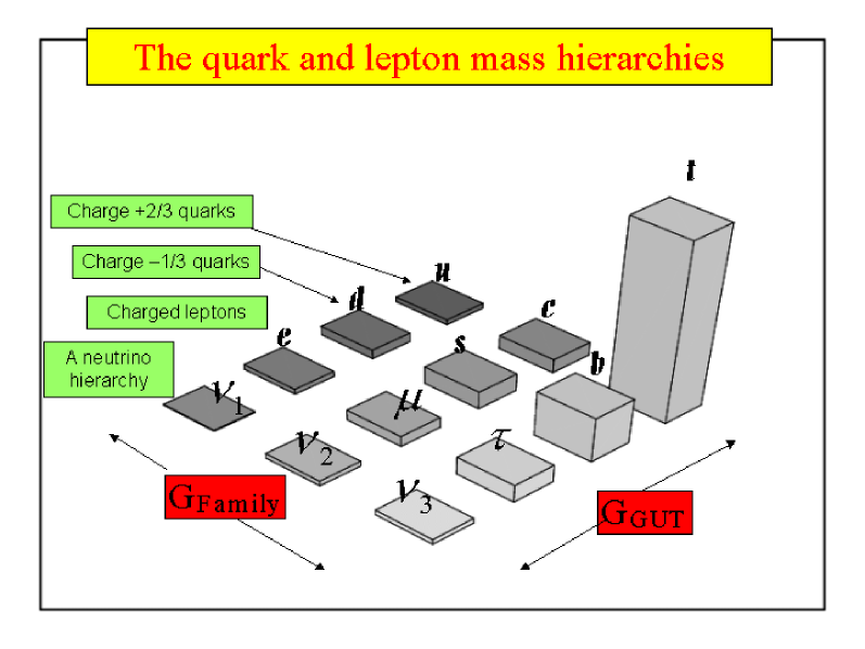
Figure 4: The fermion masses are here represented by a lego plot. We have multiplied the masses of the bottom, charm and tau by $10$, the strange and muon by $10^{2}$, the up and down by $10^{3}$, the electron by $10^{4}$ to make the lego blocks visible. It is natural to assume a normal neutrino hierarchy. We have multiplied the third neutrino mass by $10^{11}$ and the second neutrino mass by $10^{12}$ to make the lego blocks visible. This underlines how incredibly light the neutrinos are. The symmetry groups $G_{{\rm GUT}}$ and $G_{{\rm Family}}$ act in the directions indicated.

6.2 $SO(10)\times U(1)$

As an example we shall here consider a model based on a GUT group $SO(10)$ and a family symmetry $U(1)$. We shall suppose that the GUT symmetry is broken via a Pati-Salam group and define the model in terms of the subgroup $422$ [94]. This model provides an example of the use of both the $U(1)$ family symmetry to generate inter-family hierarchies, and the use of Clebsch-Gordon coefficients from the GUT group to generate intra-family structure.

The left-handed quarks and leptons are accommodated in the following 422 representations,

$${\psi^{i}}=(4,2,1)=\left(\begin{array}[]{cccc}u^{R}&u^{B}&u^{G}&\nu\\ d^{R}&d^{B}&d^{G}&e^{-}\end{array}\right)^{i}$$ (137)

$${\bar{\psi}}^{i}=(\bar{4},1,\bar{2})=\left(\begin{array}[]{cccc}\bar{d}^{R}&\bar{d}^{B}&\bar{d}^{G}&e^{+}\\ \bar{u}^{R}&\bar{u}^{B}&\bar{u}^{G}&\bar{\nu}\end{array}\right)^{i}$$ (138)

where $i=1\ldots 3$ is a family index. The Higgs fields are contained in the following representations,

$$h=(1,\bar{2},2)=\left(\begin{array}[]{cc}{h_{2}}^{+}&{h_{1}}^{0}\\ {h_{2}}^{0}&{h_{1}}^{-}\\ \end{array}\right)$$ (139)

(where $h_{1}$ and $h_{2}$ are the low energy Higgs superfields associated with the MSSM.)

The two heavy Higgs representations are

$${H}^{\alpha b}=(4,1,2)=\left(\begin{array}[]{cccc}u_{H}^{R}&u_{H}^{B}&u_{H}^{G}&\nu_{H}\\ d_{H}^{R}&d_{H}^{B}&d_{H}^{G}&e_{H}^{-}\end{array}\right)$$ (140)

and

$${\bar{H}}_{\alpha x}=(\bar{4},1,\bar{2})=\left(\begin{array}[]{cccc}\bar{d}_{H}^{R}&\bar{d}_{H}^{B}&\bar{d}_{H}^{G}&e_{H}^{+}\\ \bar{u}_{H}^{R}&\bar{u}_{H}^{B}&\bar{u}_{H}^{G}&\bar{\nu}_{H}\end{array}\right).$$ (141)

The Higgs fields are assumed to develop VEVs,

$$<H>\equiv<\nu_{H}>\sim M_{GUT},\ \ <\bar{H}>\equiv<\bar{\nu}_{H}>\sim M_{GUT}$$ (142)

leading to the symmetry breaking at $M_{GUT}$

$$\mbox{SU(4)}\otimes\mbox{SU(2)}_{L}\otimes\mbox{SU(2)}_{R}\longrightarrow\mbox{SU(3)}_{C}\otimes\mbox{SU(2)}_{L}\otimes\mbox{U(1)}_{Y}$$ (143)

in the usual notation. Under the symmetry breaking in Eq.143, the Higgs field $h$ in Eq.139 splits into two Higgs doublets $h_{1}$, $h_{2}$ whose neutral components subsequently develop weak scale VEVs,

$$<h_{1}^{0}>=v_{1},\ \ <h_{2}^{0}>=v_{2}$$ (144)

with $\tan\beta\equiv v_{2}/v_{1}$.

To construct the quark and lepton mass matrices we make use of non-renormalisable operators [122] of the form:

$$\left.i\right) \hskip 28.45274pt(\psi^{i}\bar{\psi}^{j})h\left(\frac{H\bar{H}}{M^{2}}\right)^{n}\left(\frac{\theta}{M}\right)^{p_{ij}}$$ (145)

$$\left.ii\right) \hskip 28.45274pt(\bar{\psi}^{i}\bar{\psi}^{j})\left(\frac{HH}{M^{2}}\right)\left(\frac{H\bar{H}}{M^{2}}\right)^{m}\left(\frac{\theta}{M}\right)^{q_{ij}}.$$ (146)

The $\theta$ fields are Pati-Salam singlets which carry $U(1)$ family charge and develop VEVs which break the $U(1)$ family symmetry. They are required to be present in the operators above to balance the charge of the invariant operators. After the $H$ and $\theta$ fields acquire VEVs, they generate a hierarchy in $\left.i\right)$ effective Yukawa couplings and $\left.ii\right)$ Majorana masses. These operators are assumed to originate from additional interactions at the scale $M>M_{GUT}$. The value of the powers $p_{ij}$ and $q_{ij}$ are determined by the assignment of $U(1)$ charges, with $X_{\theta}=-1$ then $p_{ij}=(X_{\psi^{i}}+X_{\bar{\psi}^{j}}+X_{h})$ and $q_{ij}=(X_{\bar{\psi}^{i}}+X_{\bar{\psi}^{j}}+X_{h})$.

The contribution to the third family Yukawa coupling is assumed to be only from the renormalisable operator with $n=p=0$ leading to Yukawa unification. The contribution of an operator, with a given power $n$, to the matrices $Y_{f=u,d,\nu,e},\,M_{RR}$ is determined by the relevant Clebsch factors coming from the gauge contractions within that operator. A list of Clebsch factors for all $n=1$ operators can be found in the appendix of [94]. These Clebsch factors give zeros for some matrices and not for others, hence a choice of operators can be made such that a large 23 entry can be given to $Y_{\nu}$ and not $Y_{u,d,e}$. We shall write,

$$\delta=\frac{<H><\bar{H}>}{M^{2}}=0.22,\ \ \epsilon=\frac{<\theta>}{M^{2}}=0.22,$$ (147)

then we can identify $\delta$ with mass splitting within generations and $\epsilon$ with splitting between generations.

The choice of $U(1)$ charges are as in [94] and can be summarised as $X_{\psi^{i}}~{}=~{}\left(1,0,0\right)$, $X_{\bar{\psi}^{i}}~{}=~{}\left(4,2,0\right)$, $X_{h}=0$, $X_{H}=0$ and $X_{\bar{H}}=0$. This fixes the powers of $\epsilon$ in each entry of the Yukawa matrix, but does not specify the complete operator. The Yukawa couplings are specified by a particular choice of operators, [123, 94] with the property

$${\cal O}\sim(H\bar{H})\sim\delta,\ \ {\cal O}^{\prime}\sim(H\bar{H})^{2}\sim\delta^{2},\ \ {\cal O}^{\prime\prime}\sim(H\bar{H})^{3}\sim\delta^{3}.$$ (148)

The Clebsch factors play an important part in determing the form of the Yukawa matrices. The particular operator choice in [94] leads to the quark and lepton mass matrices below. For example the Clebsch coeficients from the leading operator in the 22 positon gives the ratio $0:1:3$ in the $Y_{U,D,E}$ matrices. This ratio along with subleading corrections provides the correct $m_{c}:m_{s}:m_{\mu}$ ratio [124].

The final form of the Yukawa matrices is [123],

$$Y^{u} \approx \left(\begin{array}[]{lcr}\sqrt{2}\delta^{3}\epsilon^{5}&\sqrt{2}\delta^{2}\epsilon^{3}&\frac{2}{\sqrt{5}}\delta^{2}\epsilon\\ 0&\frac{8}{5\sqrt{5}}\delta^{2}\epsilon^{2}&0\\ 0&\frac{8}{5}\delta^{2}\epsilon^{2}&r_{t}\end{array}\right),$$ (152)

$$Y^{d} \approx \left(\begin{array}[]{llr}\frac{8}{5}\delta\epsilon^{5}&-\sqrt{2}\delta^{2}\epsilon^{3}&\frac{4}{\sqrt{5}}\delta^{2}\epsilon\\ \frac{2}{\sqrt{5}}\delta\epsilon^{4}&\left[\sqrt{\frac{2}{5}}\delta\epsilon^{2}+\frac{16}{5\sqrt{5}}\delta^{2}\epsilon^{2}\right]&\sqrt{\frac{2}{5}}\delta^{2}\\ \frac{8}{5}\delta\epsilon^{5}&\sqrt{2}\delta\epsilon^{2}&r_{b}\end{array}\right),$$ (156)

$$Y^{e} \approx \left(\begin{array}[]{llr}\frac{6}{5}\delta\epsilon^{5}&0&0\\ \frac{4}{\sqrt{5}}\delta\epsilon^{4}&\left[-3\sqrt{\frac{2}{5}}\delta\epsilon^{2}+\frac{12}{5\sqrt{5}}\delta^{2}\epsilon^{2}\right]&-3\sqrt{\frac{2}{5}}\delta^{2}\\ \frac{6}{5}\delta\epsilon^{5}&\sqrt{2}\delta\epsilon^{2}&1\end{array}\right),$$ (160)

$$Y^{\nu} \approx \left(\begin{array}[]{llr}\sqrt{2}\delta^{3}\epsilon^{5}&{2}\delta\epsilon^{3}&0\\ 0&\frac{6}{5\sqrt{5}}\delta^{2}\epsilon^{2}&2\delta\\ 0&\frac{6}{5}\delta^{2}\epsilon^{2}&r_{\nu}\end{array}\right),$$ (164)

where the numerical Clebsch factors are displayed explicitly, and $r_{t},r_{b},r_{\nu}$ are order unity parameters which quantify the deviations from exact Yukawa unification [123], but all other order unity coefficients have been dropped.

The Majorana operators are assumed to arise from an $m=0$ operator in the 33 position and $m=1$ operators elsewhere, resulting in

$$M_{RR}\approx\left(\begin{array}[]{ccr}\delta\epsilon^{8}&\delta\epsilon^{6}&\delta\epsilon^{4}\\ \delta\epsilon^{6}&\delta\epsilon^{4}&\delta\epsilon^{2}\\ \delta\epsilon^{4}&\delta\epsilon^{2}&1\end{array}\right)M_{3}.$$ (165)

In the neutrino sector the matrices above satisfy the condition of sequential dominance in which a neutrino mass hierarchy naturally results with the heaviest (third) right-handed neutrino being mainly responsible for the atmospheric neutrino mass, and the second heaviest right-handed neutrino being mainly responsible for the solar neutrino mass. Thus this model corresponds to HSDa in Table 2. Using the HSDa ordering in Table 2 with the matrices in Eqs.164,165 we can use the analytic results in Eqs.61-66 to give estimates of neutrino masses

$$m_{1} \sim {\delta^{5}}{\epsilon^{2}}\frac{v_{2}^{2}}{M_{3}}$$ (166)

$$m_{2} \approx \frac{4\delta\epsilon^{2}}{s_{12}^{2}}\frac{v_{2}^{2}}{M_{3}}$$ (167)

$$m_{3} \approx (4\delta^{2}+r_{\nu}^{2})\frac{v_{2}^{2}}{M_{3}}$$ (168)

and neutrino mixing angles:

$$\tan\theta_{23}^{\nu} \approx \frac{2\delta}{r_{\nu}}$$ (169)

$$\tan\theta_{12}^{\nu} \approx \frac{2}{\left(c_{23}\frac{6}{5\sqrt{2}}-s_{23}\frac{6}{5}\right)}\frac{\epsilon}{\delta}$$ (170)

$$\theta_{13}^{\nu} \approx \frac{\frac{12}{5}\delta^{2}\epsilon\left(\frac{2\delta}{\sqrt{5}}+r_{\nu}\right)}{\left((2\delta)^{2}+r_{\nu}^{2}\right)^{3/2}}$$ (171)

which are a good fit to the LMA MSW solution for $\epsilon$ and $\delta$ as in Eq.147.

6.3 $SO(10)\times SU(3)$

As an example of a model based on a non-Abelian family symmetry, we briefly review the model proposed in [96]. The model uses the largest family symmetry $SU(3)$ consistent with $SO(10)$ GUTs. An important further motivation for $SU(3)$ family symmetry is, in the framework of sequential dominance, to relate the second and third entries of the Yukawa matrix, as required to obtain an almost maximal 23 mixing in the atmospheric neutrino sector [95]. In this framework we already saw that the theoretical requirements that the neutrino Yukawa matrix resembles the quark Yukawa matrices, and therefore has a large 33 element with no large off-diagonal elements and a texture zero in the 11 position [45], leads uniquely to LSDa in Table 2, where the dominant right-handed neutrino is the first (lightest) one. Assuming this then the atmospheric neutrino mixing angle is given by $\tan\theta_{23}^{\nu}\approx Y^{\nu}_{21}/Y^{\nu}_{31}\approx 1$. The sequential dominance conditions which were assumed in Eq.58 will here be derived from the symmetries of the model. Thus this model provides an example of the application of sequential dominance to realistic models of flavour, and shows how the conditions of sequential dominance which were simply assumed earlier can motivate models based on GUTs and family symmetry which are capable of explaining these conditions. In other words, the conditions for sequential dominance can provide clues to the nature of the underlying flavour theory.

The starting point of the model is the observation that an excellent fit to all quark data is given by the approximately symmetric form of quark Yukawa matrices [65]

$$Y^{u}\propto\left(\begin{array}[]{ccc}0&\epsilon^{3}&O(\epsilon^{3})\\ .&\epsilon^{2}&O(\epsilon^{2})\\ .&.&1\end{array}\right),\ \ \ \ Y^{d}\propto\left(\begin{array}[]{crc}0&1.5\bar{\epsilon}^{3}&0.4\bar{\epsilon}^{3}\\ .&\bar{\epsilon}^{2}&1.3\bar{\epsilon}^{2}\\ .&.&1\end{array}\right)$$ (172)

where the expansion parameters $\epsilon$ and $\bar{\epsilon}$ are given by

$$\epsilon\approx 0.05,\ \ \bar{\epsilon}\approx 0.15.$$ (173)

This motivates a particular model in which the three families are unified as triplets under an $SU(3)$ family symmetry, and $16^{\prime}s$ under an $SO(10)$ GUT [95, 107, 96],

$$\psi_{i}=(3,16),$$ (174)

where as before the $SO(10)$ is broken via the Pati-Salam group giving the equivalent 422 reps in Eqs.137,138,

$${\psi_{i}}=(3,4,2,1),\ \ {\bar{\psi}}_{i}=(3,\bar{4},1,\bar{2}).$$ (175)

Further symmetries $R\times Z_{2}\times U(1)$ are assumed to ensure that the vacuum alignment leads to a universal form of Dirac mass matrices for the neutrinos, charged leptons and quarks [96]. To build a viable model we also need spontaneous breaking of the family symmetry

$$SU(3)\longrightarrow SU(2)\longrightarrow{\rm Nothing}$$ (176)

To achieve this symmetry breaking additional Higgs fields $\phi_{3},$ $\overline{\phi}_{3},$ $\phi_{23}$ and $\overline{\phi}_{23}$ are required. The largeness of the third family fermion masses implies that $SU(3)$ must be strongly broken by new Higgs antitriplet fields $\phi_{3}$ which develop a vev in the third $SU(3)$ component $<\phi_{3}>^{T}=(0,0,a_{3})$ as in [95]. $\phi_{3}^{i}$ transforms under $SU(2)_{R}$ as ${\bf 3\oplus 1}$ rather than being $SU(2)_{R}$ singlets as assumed in [95], and develops vevs in the $SU(3)\times SU(2)_{R}$ directions

$$<\phi_{3}>=<\overline{\phi_{3}}>=\left(\begin{array}[]{c}0\\ 0\\ 1\end{array}\right)\otimes\left(\begin{array}[]{cc}a_{3}^{u}&0\\ 0&a_{3}^{d}\end{array}\right).$$ (177)

The symmetry breaking also involves the $SU(3)$ antitriplets $\phi_{23}$ which develop vevs [95]

$$<\phi_{23}>=\left(\begin{array}[]{c}0\\ 1\\ 1\end{array}\right)b,$$ (178)

where, as in [95], vacuum alignment ensures that the vevs are aligned in the 23 direction. Due to D-flatness there must also be accompanying Higgs triplets such as $\overline{\phi_{23}}$ which develop vevs [95]

$$<\overline{\phi_{23}}>=\left(\begin{array}[]{c}0\\ 1\\ 1\end{array}\right)b.$$ (179)

We also introduce an adjoint $\Sigma$ field which develops vevs in the $SU(4)_{PS}\times SU(2)_{R}$ direction which preserves the hypercharge generator $Y=T_{3R}+(B-L)/2$, and implies that any coupling of the $\Sigma$ to a fermion and a messenger such as $\Sigma^{a\alpha}_{b\beta}\psi^{c}_{a\alpha}\chi^{b\beta}$, where the $SU(2)_{R}$ and $SU(4)_{PS}$ indices have been displayed explicitly, is proportional to the hypercharge $Y$ of the particular fermion component of $\psi^{c}$ times the vev $\sigma$. In addition a $\theta$ field is required for the construction of Majorana neutrino masses.

The leading operators allowed by the symmetries are

$$P_{{\rm Yuk}} \sim \frac{1}{M^{2}}\psi_{i}\phi_{3}^{i}\bar{\psi}_{j}\phi_{3}^{j}h$$ (180)

$$+ \frac{\Sigma}{M^{3}}\psi_{i}\phi_{23}^{i}\bar{\psi}_{j}\phi_{23}^{j}h$$ (181)

$$P_{{\rm Maj}} \sim \frac{1}{M}\bar{\psi}_{i}\theta^{i}\theta^{j}\bar{\psi}_{j}$$ (182)

where the operator mass scales, generically denoted by $M$ may differ and we have suppressed couplings of $O(1).$

The final form of the Yukawa matrices and heavy Majorana matrix after inserting a particular choice of order unity coefficients is [96]

$$Y^{u} \approx \left(\begin{array}[]{llr}0&1.2\epsilon^{3}&0.9\epsilon^{3}\\ -1.2\epsilon^{3}&-\frac{2}{3}\epsilon^{2}&-\frac{2}{3}\epsilon^{2}\\ -0.9\epsilon^{3}&-\frac{2}{3}\epsilon^{2}&1\end{array}\right)\bar{\epsilon},$$ (186)

$$Y^{d} \approx \left(\begin{array}[]{llr}0&1.6\bar{\epsilon}^{3}&0.7\bar{\epsilon}^{3}\\ -1.6\bar{\epsilon}^{3}&\bar{\epsilon}^{2}&\bar{\epsilon}^{2}+\bar{\epsilon}^{\frac{5}{2}}\\ -0.7\bar{\epsilon}^{3}&\bar{\epsilon}^{2}&1\end{array}\right)\bar{\epsilon},$$ (190)

$$Y^{e} \approx \left(\begin{array}[]{llr}0&1.6\bar{\epsilon}^{3}&0.7\bar{\epsilon}^{3}\\ -1.6\bar{\epsilon}^{3}&3\bar{\epsilon}^{2}&3\bar{\epsilon}^{2}\\ -0.7\bar{\epsilon}^{3}&3\bar{\epsilon}^{2}&1\end{array}\right)\bar{\epsilon},$$ (194)

$$Y^{\nu} \approx \left(\begin{array}[]{llr}0&1.2\epsilon^{3}&0.9\epsilon^{3}\\ -1.2\epsilon^{3}&-\alpha\epsilon^{2}&-\alpha\epsilon^{2}\\ -0.9\epsilon^{3}&-\alpha\epsilon^{2}-\epsilon^{3}&1\end{array}\right)\bar{\epsilon}.$$ (198)

$$M_{RR}\approx\left(\begin{array}[]{ccr}\epsilon^{6}\bar{\epsilon}^{3}&0&0\\ 0&\epsilon^{6}\bar{\epsilon}^{2}&0\\ 0&0&1\end{array}\right)M_{3}.$$ (199)

The model gives excellent agreement with the quark and lepton masses and mixing angles. For the up and down quarks the form of $Y^{u}$ and $Y^{d}$ given in Eq.186, 190 is consistent with the phenomenological fit in Eq.172. The charged lepton mass matrix is of the Georgi-Jarslkog [124] form which, after including radiative corrections, gives an excellent description of the charged lepton masses. In the neutrino sector the parameters satisfy the conditions of sequential dominance 58, with the lightest right-handed neutrino giving the dominant contribution to the heaviest physical neutrino mass, and the second right-handed neutrino giving the leading subdominant contribution, providing that $\alpha\sim\epsilon$. It thus falls into the category of LSDa in Table 2.

Analytic estimates of neutrino masses and mixing angles for sequential dominance were derived in [26], and for the special case here of LSDa, with the 11 neutrino Yukawa coupling equal to zero, they are given in Eqs.61-66 from which the analytic estimates below for the neutrino masses are obtained,

$$m_{1} \sim \bar{\epsilon}^{2}\frac{v_{2}^{2}}{M_{3}}$$ (200)

$$m_{2} \approx 5.8\frac{v_{2}^{2}}{M_{3}}$$ (201)

$$m_{3} \approx 15\frac{v_{2}^{2}}{M_{3}}$$ (202)

and neutrino mixing angles:

$$\tan\theta_{23}^{\nu} \approx 1.3$$ (203)

$$\tan\theta_{12}^{\nu} \approx 0.66$$ (204)

$$\theta_{13}^{\nu} \approx 1.6\bar{\epsilon}$$ (205)

Note that the physical lepton mixing angle $\theta_{13}$ receives a large contribution from the neutrino sector $\theta_{13}^{\nu}\sim 0.3$ at the high energy scale, for this choice of parameters, compared to the current CHOOZ limit $\theta_{13}\leq 0.2$ [14]. However the physical mixing angles will receive charged lepton contributions [26] and all the parameters are subject to radiative corrections in running from the high energy scale to low energies, although in sequential dominance models these corrections are only a few per cent [121]. Thus the model predicts that $\theta_{13}$ is close to the current CHOOZ limit, and could be observed by the next generation of long baseline experiments such as MINOS or OPERA.

7 Conclusions

This focus of the review has been on “mainstream” neutrino mass models, defined as see-saw models involving three active neutrinos which are capable of describing both the atmospheric neutrino oscillation data, and the LMA MSW solar solution, which is now uniquely specified by recent data. We have briefly reviewed the current experimental status, showed how to parametrise and construct the neutrino mixing matrix, and presented the leading order neutrino Majorana mass matrices. We then introduced the see-saw mechanism, and discussed a natural application of it to current data using the sequential dominance mechanism, which we compared to an early proposal for obtaining large mixing angles. We showed how both the Standard Model and the Minimal Supersymmetric Standard Model may be extended to incorporate the see-saw mechanism, and showed how the latter case leads to the expectation of lepton flavour violation. The see-saw mechanism motivates models with additional symmetries such as unification and family symmetry models, and we tabulated some possible models, before focussing on two particular models based on $SO(10)$ grand unification and either $U(1)$ or $SU(3)$ family symmetry as specific examples. We have provided extensive appendices which include techniques for analytically diagonalising different types of mass matrices involving two large mixing angles and one small mixing angle, to leading order in the small mixing angle.

Neutrino physics has witnessed a renaissance period with the watershed provided by Super-Kamiokande in 1998. Before then we did not know whether atmospheric and solar neutrino oscillations were fact or fancy. Now we know they are fact whose explanation requires two large mixing angles. We have seen in this review that there is no shortage of theoretical models which can account for these data. Even discounting those theoretical models which predicted a small solar angle, or vacuum oscillation mass splittings, there are many many models that can describe the current data. In this review we have tried to emphasise useful approaches and techniques, rather than giving a detailed catalogue of all possible models. We make no apology for emphasising the see-saw mechanism, which is probably the most elegant way of accounting for small neutrino masses. We have further shown that the see-saw mechanism may be successfully applied to the atmospheric and solar data to yield a neutrino mass hierarchy and two large mixing angles in a technically natural and elegant way using the idea of sequential dominance. Sequential dominance requires certain mild conditions to apply, and we have seen that these conditions may in turn arise from the symmetries of realistic models.

The problem of neutrino masses and mixings should be addressed in the wider context of the problem of all quark and lepton masses and mixing angles, and in this wider context we have emphasised ideas such as unification and family symmetry which will surely play a role in the ultimate solution to the problem of flavour. In Table 3 we have classified successful models according to the different unification and family symmetries upon which they are based. It remains to be seen if any of these models will turn out to provide the solution to the problem of flavour. If this turns out to be not the case, then the effort will not have been in vain, since it is quite likely that some of the ideas on which these models are based will survive. Here we have emphasised particularly promising ideas such as the see-saw mechanism, sequential dominance, supersymmetry, unification and family symmetry, which when combined with the neutrino data could help to unlock the whole mystery of flavour.

Acknowledgements

I would like to thank Stefan Antusch for reading the manuscript and PPARC for the support of a Senior Fellowship.

Appendix A Equivalence of different parametrisations

In this appendix we exhibit the equivalence of different parametrisations of the lepton mixing matrix. A $3\times 3$ unitary matrix may be parametrised by 3 angles and 6 phases. We shall find it convenient to parametrise a unitary matrix $V^{\dagger}$ by :

$$V^{\dagger}=P_{2}R_{23}R_{13}P_{1}R_{12}P_{3}$$ (206)

where $R_{ij}$ are a sequence of real rotations corresponding to the Euler angles $\theta_{ij}$, and $P_{i}$ are diagonal phase matrices. The Euler matrices are given by

$$R_{23}=\left(\begin{array}[]{ccc}1&0&0\\ 0&c_{23}&s_{23}\\ 0&-s_{23}&c_{23}\\ \end{array}\right)$$ (207)

$$R_{13}=\left(\begin{array}[]{ccc}c_{13}&0&s_{13}\\ 0&1&0\\ -s_{13}&0&c_{13}\\ \end{array}\right)$$ (208)

$$R_{12}=\left(\begin{array}[]{ccc}c_{12}&s_{12}&0\\ -s_{12}&c_{12}&0\\ 0&0&1\\ \end{array}\right)$$ (209)

where $c_{ij}=\cos\theta_{ij}$ and $s_{ij}=\sin\theta_{ij}$. The phase matrices are given by

$$P_{1}=\left(\begin{array}[]{ccc}1&0&0\\ 0&e^{i\chi}&0\\ 0&0&1\end{array}\right)$$ (210)

$$P_{2}=\left(\begin{array}[]{ccc}1&0&0\\ 0&e^{i\phi_{2}}&0\\ 0&0&e^{i\phi_{3}}\end{array}\right)$$ (211)

$$P_{3}=\left(\begin{array}[]{ccc}e^{i\omega_{1}}&0&0\\ 0&e^{i\omega_{2}}&0\\ 0&0&e^{i\omega_{3}}\end{array}\right)$$ (212)

By commuting the phase matrices to the left, it is not difficult to show that the parametrisation in Eq.206 is equivalent to

$$V^{\dagger}=PU_{23}U_{13}U_{12}$$ (213)

where $P=P_{1}P_{2}P_{3}$ and

$$U_{23}=\left(\begin{array}[]{ccc}1&0&0\\ 0&c_{23}&s_{23}e^{-i\delta_{23}}\\ 0&-s_{23}e^{i\delta_{23}}&c_{23}\\ \end{array}\right)$$ (214)

$$U_{13}=\left(\begin{array}[]{ccc}c_{13}&0&s_{13}e^{-i\delta_{13}}\\ 0&1&0\\ -s_{13}e^{i\delta_{13}}&0&c_{13}\\ \end{array}\right)$$ (215)

$$U_{12}=\left(\begin{array}[]{ccc}c_{12}&s_{12}e^{-i\delta_{12}}&0\\ -s_{12}e^{i\delta_{12}}&c_{12}&0\\ 0&0&1\\ \end{array}\right)$$ (216)

where

$$\delta_{23}=\chi+\omega_{2}-\omega_{3}$$ (217)

$$\delta_{13}=\omega_{1}-\omega_{3}$$ (218)

$$\delta_{12}=\omega_{1}-\omega_{2}$$ (219)

The matrix $U$ is an example of a unitary matrix, and as such it may be parametrised by either of the equivalent forms in Eqs.206 or 213. If we use the form in Eq.213 then the phase matrix $P$ on the left may always be removed by an additional charged lepton phase rotation $\Delta V^{E_{L}}=P^{\dagger}$, which is always possible since right-handed charged lepton phase rotations can always make the charged lepton masses real. Therefore $U$ can always be parametrised by

$$U=U_{23}U_{13}U_{12}$$ (220)

which involves just three irremoveable physical phases $\delta_{ij}$. In this parametrisation the Dirac phase $\delta$ which enters the CP odd part of neutrino oscillation probabilities is given by

$$\delta=\delta_{13}-\delta_{23}-\delta_{12}.$$ (221)

Another common parametrisation of the lepton mixing matrix is

$$U=R_{23}U_{13}R_{12}P_{0}$$ (222)

where

$$P_{0}=\left(\begin{array}[]{ccc}e^{i\beta_{1}}&0&0\\ 0&e^{i\beta_{2}}&0\\ 0&0&1\end{array}\right)$$ (223)

and in Eq.222 $U_{13}$ is of the form in Eq.215 but with $\delta_{13}$ replaced by the Dirac phase $\delta$. The parametrisation in Eq.222 can be transformed into the parametrisation in Eq.220 by commuting the phase matrix $P_{0}$ in Eq.222 to the left, and then removing the phases on the left-hand side by charged lepton phase rotations. The two parametrisations are then related by the phase relations

$$\delta_{23}=\beta_{2}$$ (224)

$$\delta_{13}=\delta+\beta_{1}$$ (225)

$$\delta_{12}=\beta_{1}-\beta_{2}$$ (226)

The use of the parametrisation in Eq.222 is widespread in the literature, however for the reasons discussed in the next sub-section we prefer to use the parametrisation in Eq.220 which is trivially related to Eq.222 by the above phase relations.

Appendix B Three Family Oscillation Formulae

At a Neutrino Factory it is relatively straightforward to measure the angle $\theta_{13}$ using the Golden Signature of “wrong sign” muons. The effect relies on the full three family oscillation formulae which we discuss in this Appendix. For example suppose there are positive muons circulating in the storage ring, then these decay as $\mu^{+}\rightarrow e^{+}\nu_{e}\bar{\nu}_{\mu}$ giving a mixed beam of electron neutrinos and muon anti-neutrinos. The muon anti-neutrinos will interact in the far detector to produce positive muons. Any “wrong sign” negative muons which may be observed can only arise from the neutrino oscillation of electron neutrinos into muon neutrinos with probability given by a CP conserving part $P^{+}$ and a a CP violating part $P^{-}$. The exact formulae in vacuum are given by:

$$P(\nu_{e}\rightarrow\nu_{\mu})=P^{+}(\nu_{e}\rightarrow\nu_{\mu})+P^{-}(\nu_{e}\rightarrow\nu_{\mu})$$ (227)

$$P(\bar{\nu}_{e}\rightarrow\bar{\nu}_{\mu})=P^{+}(\bar{\nu}_{e}\rightarrow\bar{\nu}_{\mu})+P^{-}(\bar{\nu}_{e}\rightarrow\bar{\nu}_{\mu})$$ (228)

where the CP conserving parts are

$$P^{+}(\nu_{e}\rightarrow\nu_{\mu})=P^{+}(\bar{\nu}_{e}\rightarrow\bar{\nu}_{\mu})= - 4Re(U_{e1}U_{\mu 1}^{*}U_{e2}^{*}U_{\mu 2})\sin^{2}(1.27\Delta m_{21}^{2}L/E)$$ (229)

$$- 4Re(U_{e1}U_{\mu 1}^{*}U_{e3}^{*}U_{\mu 3})\sin^{2}(1.27\Delta m_{31}^{2}L/E)$$

$$- 4Re(U_{e2}U_{\mu 2}^{*}U_{e3}^{*}U_{\mu 3})\sin^{2}(1.27\Delta m_{32}^{2}L/E)$$

and the CP violating parts are

$$P^{-}(\nu_{e}\rightarrow\nu_{\mu})=-P^{-}(\bar{\nu}_{e}\rightarrow\bar{\nu}_{\mu})=-c_{13}\sin 2\theta_{13}\sin 2\theta_{12}\sin 2\theta_{23}\sin\delta$$ (230)

$$\times \sin(1.27\Delta m_{21}^{2}L/E)\sin(1.27\Delta m_{31}^{2}L/E)\sin(1.27\Delta m_{32}^{2}L/E)$$

Note that $P^{-}$ requires all three families to contribute, and it vanishes if any mixing angle or mass splitting is zero. The angle $\theta_{13}$ may easily be extracted from $U_{e3}$ in the dominant CP conserving term $P^{+}$.

In order to determine the CP violating phase $\sin\delta$ it is necessary to measure the CP violating term $P^{-}$. In order to do this one must compare the result for $P(\nu_{e}\rightarrow\nu_{\mu})$ to the result to the case where the positive muons in the storage ring are replaced by negative muons and the analagous experiment is performed to measure $P(\bar{\nu}_{e}\rightarrow\bar{\nu}_{\mu})$. The CP violating asymmetry due to the CP violating phase $\delta$ is given by

$$A^{\delta}=\frac{P(\nu_{e}\rightarrow\nu_{\mu})-P(\bar{\nu}_{e}\rightarrow\bar{\nu}_{\mu})}{P(\nu_{e}\rightarrow\nu_{\mu})+P(\bar{\nu}_{e}\rightarrow\bar{\nu}_{\mu})}$$ (231)

from which we obtain

$$A^{\delta}=\frac{P^{-}(\nu_{e}\rightarrow\nu_{\mu})}{P^{+}(\nu_{e}\rightarrow\nu_{\mu})}\approx\frac{\sin 2\theta_{12}\sin\delta}{\sin\theta_{13}}\sin(1.27\Delta m_{21}^{2}L/E)$$ (232)

It is clear that in order to measure the CP asymmetry we require large $\theta_{12}$ and large $\Delta m_{21}^{2}$ and this corresponds to the LMA MSW solution. In addition we require large $\sin\delta$. Also it would seem that having small $\theta_{13}$ enhances the CP asymmetry, however it should be remembered that the CP asymmetric rate $P^{-}$ in Eq.230 is proportional to $\sin 2\theta_{13}$, and so $\theta_{13}$ should not be too small otherwise the number of events will be too small.

Unfortunately life is not quite as simple as the above discussion portrays. The Earth is made from matter and not anti-matter and so CP will be violated by matter effects as the neutrino beam passes through the Earth from the muon storage ring to the far detector. For example the matter effects will modify the formulas for $P(\nu_{e}\rightarrow\nu_{\mu})$ involving $\theta_{13}$ and $\Delta m_{31}^{2}$ as follows:

$$\sin 2\theta_{13} \rightarrow \frac{\sin 2\theta_{13}}{\left(\frac{A}{\Delta m_{31}^{2}}-\cos 2\theta_{13}\right)^{2}+\sin^{2}2\theta_{13}}$$

$$\Delta m_{31}^{2} \rightarrow \Delta m_{31}^{2}\sqrt{\left(\frac{A}{\Delta m_{31}^{2}}-\cos 2\theta_{13}\right)^{2}+\sin^{2}2\theta_{13}}$$ (233)

where

$$A=7.6\times 10^{-5}\rho E$$ (234)

where $\rho$ is the density of the Earth in gcm^-3 and $E$ is the beam energy in GeV. The point is that for $P(\bar{\nu}_{e}\rightarrow\bar{\nu}_{\mu})$ the sign of $A$ is reversed. From one point of view this is good news, since unlike the vacuum oscillation formulae, $\Delta m_{31}^{2}$ enters linearly, not quadratically, and so matter effects enable the sign of the mass squared splitting to be determined in a rather straightforward way.

However from the point of view of measuring $\sin\delta$ it leads to complications since the asymmetry in the rate in Eq.231 can get contributions from both intrinsic CP violation and from matter induced CP violation, and the measured asymmetry is a sum of the two effects

$$A^{CP}=A^{\delta}+A^{matter}$$ (235)

Since both effects are by themselves rather small, it will be a very difficult job to disentangle them, and the optimal strategy continues to be studied [19]. The optimal place to sit in order to observe CP violation seems to be at the peak of $\sin(1.27\Delta m_{32}^{2}L/E)$ in order to maximise $P^{-}$ according to Eq.230 (certainly we should avoid being at its node otherwise CP violation vanishes). In order to do this efficiently it may be desirable to have energy-tunable beams, and it is certainly necessary to have a good understanding of the density profile of the Earth. Assuming the LMA solution, the prospects for measuring CP violation at a Neutrino Factory are good.

Appendix C Charged lepton contributions to the lepton mixing matrix

In this appendix we discuss the contribution of the charged lepton mixing angles to the lepton mixing matrix. The lepton mixing matrix is constructed in Eq.23 as a product of a unitary matrix from the charged lepton sector $V^{E_{L}}$ and a unitary matrix from the neutrino sector ${V^{\nu_{L}}}^{\dagger}$. Each of these unitary matrices may be parametrised by the parametrisation of $V^{\dagger}$ in Eq.206. Thus we write

$${V^{\nu_{L}}}^{\dagger}=P_{2}^{\nu_{L}}R_{23}^{\nu_{L}}R_{13}^{\nu_{L}}P_{1}^{\nu_{L}}R_{12}^{\nu_{L}}P_{3}^{\nu_{L}}$$ (236)

$${V^{E_{L}}}^{\dagger}=P_{2}^{E_{L}}R_{23}^{E_{L}}R_{13}^{E_{L}}P_{1}^{E_{L}}R_{12}^{E_{L}}P_{3}^{E_{L}}$$ (237)

where the Euler angles and phases are defined as in Eqs.207-212 but now there are independent angles and phases for the left-handed neutrino and charged lepton sectors distinguished by the superscripts $\nu_{L}$ and $E_{L}$. The lepton mixing matrix from Eqs.23,236,237 is then

$$U={P_{3}^{E_{L}}}^{\dagger}{R_{12}^{E_{L}}}^{\dagger}{P_{1}^{E_{L}}}^{\dagger}{R_{13}^{E_{L}}}^{\dagger}{R_{23}^{E_{L}}}^{\dagger}{P_{2}^{E_{L}}}^{\dagger}P_{2}^{\nu_{L}}R_{23}^{\nu_{L}}R_{13}^{\nu_{L}}P_{1}^{\nu_{L}}R_{12}^{\nu_{L}}P_{3}^{\nu_{L}}$$ (238)

As before we commute all the phase matrices to the left, then choose ${P_{3}^{E_{L}}}^{\dagger}$ to cancel all the phases on the left-hand side, to leave just

$$U={U_{12}^{E_{L}}}^{\dagger}{U_{13}^{E_{L}}}^{\dagger}{U_{23}^{E_{L}}}^{\dagger}U_{23}^{\nu_{L}}U_{13}^{\nu_{L}}U_{12}^{\nu_{L}}$$ (239)

with independent phases and angles for the left-handed neutrino and charged lepton sectors, in the convention of Eqs.214,215,216. The phases in Eq.239 are given in terms of the phases in Eqs.236, 237 by

$$\delta_{12}^{\nu_{L}} = \omega_{1}^{\nu_{L}}-\omega_{2}^{\nu_{L}}$$ (240)

$$\delta_{13}^{\nu_{L}} = \omega_{1}^{\nu_{L}}-\omega_{3}^{\nu_{L}}$$ (241)

$$\delta_{23}^{\nu_{L}} = \chi^{\nu_{L}}+\omega_{2}^{\nu_{L}}-\omega_{3}^{\nu_{L}}$$ (242)

$$\delta_{23}^{E_{L}} = -\phi_{2}^{E_{L}}+\phi_{3}^{E_{L}}+\phi_{2}^{\nu_{L}}-\phi_{3}^{\nu_{L}}+\chi^{\nu_{L}}+\omega_{2}^{\nu_{L}}-\omega_{3}^{\nu_{L}}$$ (243)

$$\delta_{13}^{E_{L}} = \phi_{3}^{E_{L}}-\phi_{3}^{\nu_{L}}+\omega_{1}^{\nu_{L}}-\omega_{3}^{\nu_{L}}$$ (244)

$$\delta_{12}^{E_{L}} = \chi^{E_{L}}+\phi_{2}^{E_{L}}-\phi_{2}^{\nu_{L}}-\chi^{\nu_{L}}+\omega_{1}^{\nu_{L}}-\omega_{2}^{\nu_{L}}$$ (245)

The form of $U$ in Eq.239 is similar to the parametrisation in Eq.31, which is the practical reason why we prefer that form rather than that in Eq.222.

We now discuss the lepton mixing matrix to leading order in $\theta_{13}$. From Eqs.220,214,215,216, we find to leading order in $\theta_{13}$ that $U$ may be expanded as:

$$U\approx$$

$$\left(\begin{array}[]{ccc}c_{12}&s_{12}e^{-i\delta_{12}}&\theta_{13}e^{-i\delta_{13}}\\ -s_{12}c_{23}e^{i\delta_{12}}-c_{12}s_{23}\theta_{13}e^{i(\delta_{13}-\delta_{23})}&c_{12}c_{23}-s_{12}s_{23}\theta_{13}e^{i(-\delta_{23}+\delta_{13}-\delta_{12})}&s_{23}e^{-i\delta_{23}}\\ s_{12}s_{23}e^{i(\delta_{23}+\delta_{12})}-c_{12}c_{23}\theta_{13}e^{i\delta_{13}}&-c_{12}s_{23}e^{i\delta_{23}}-s_{12}c_{23}\theta_{13}e^{i(\delta_{13}-\delta_{12})}&c_{23}\\ \end{array}\right)$$ (249)

(250)

For $\theta_{13}=0.1$, close to the CHOOZ limit, the approximate form in Eq.250 is accurate to 1%.

We now wish to expand the MNS matrix in terms of neutrino and charged lepton mixing angles and phases to leading order in small angles, using Eq.239. In technically natural theories, based on right-handed neutrino dominance, the contribution to $\theta_{23}$ comes mainly from the neutrino sector, $\theta_{23}\approx\theta_{23}^{\nu_{L}}$. Furthermore in natural theories we expect that the contributions to $\theta_{13}$ are all separately small so that the smallness of this angle does not rely on accidental cancellations. Clearly this implies that $\theta_{13}^{\nu_{L}}$ and $\theta_{13}^{E_{L}}$ must both be $\stackrel{{\scriptstyle<}}{{{}_{\sim}}}\theta_{13}$. Since the 13 element of $U$ also receives a contribution from the charged lepton sector proportional to $s_{12}^{E_{L}}s_{23}^{\nu_{L}}$, the same argument also implies that $\theta_{12}^{E_{L}}\stackrel{{\scriptstyle<}}{{{}_{\sim}}}\theta_{13}$. Therefore the natural expectation is that all the charged lepton mixing angles are small! Expanding Eq.239 to leading order in small angles $\theta_{12}^{E_{L}}$, $\theta_{23}^{E_{L}}$, $\theta_{13}^{E_{L}}$, $\theta_{13}^{\nu_{L}}$, we find

$$U\approx$$

$$\left(\begin{array}[]{ccc}c_{12}^{\nu_{L}}&s_{12}^{\nu_{L}}e^{-i\delta_{12}^{\nu_{L}}}&\theta_{13}^{\nu_{L}}e^{-i\delta_{13}^{\nu_{L}}}\\ -s_{12}^{\nu_{L}}c_{23}^{\nu_{L}}e^{i\delta_{12}^{\nu_{L}}}-c_{12}^{\nu_{L}}s_{23}^{\nu_{L}}\theta_{13}^{\nu_{L}}e^{i(\delta_{13}^{\nu_{L}}-\delta_{23}^{\nu_{L}})}&c_{12}^{\nu_{L}}c_{23}^{\nu_{L}}-s_{12}^{\nu_{L}}s_{23}^{\nu_{L}}\theta_{13}^{\nu_{L}}e^{i(-\delta_{23}^{\nu_{L}}+\delta_{13}^{\nu_{L}}-\delta_{12}^{\nu_{L}})}&s_{23}^{\nu_{L}}e^{-i\delta_{23}^{\nu_{L}}}\\ s_{12}^{\nu_{L}}s_{23}^{\nu_{L}}e^{i(\delta_{23}^{\nu_{L}}+\delta_{12}^{\nu_{L}})}-c_{12}^{\nu_{L}}c_{23}^{\nu_{L}}\theta_{13}^{\nu_{L}}e^{i\delta_{13}^{\nu_{L}}}&-c_{12}^{\nu_{L}}s_{23}^{\nu_{L}}e^{i\delta_{23}^{\nu_{L}}}-s_{12}^{\nu_{L}}c_{23}^{\nu_{L}}\theta_{13}^{\nu_{L}}e^{i(\delta_{13}^{\nu_{L}}-\delta_{12}^{\nu_{L}})}&c_{23}^{\nu_{L}}\\ \end{array}\right)$$

$$+\theta_{23}^{E_{L}}\left(\begin{array}[]{ccc}c_{12}^{\nu_{L}}&s_{12}^{\nu_{L}}e^{-i\delta_{12}^{\nu_{L}}}&0\\ -s_{23}^{\nu_{L}}s_{12}^{\nu_{L}}e^{i(\delta_{23}^{\nu_{L}}-\delta_{23}^{E_{L}}+\delta_{12}^{\nu_{L}})}&s_{23}^{\nu_{L}}c_{12}^{\nu_{L}}e^{i(\delta_{23}^{\nu_{L}}-\delta_{23}^{E_{L}})}&-c_{23}^{\nu_{L}}e^{-i\delta_{23}^{E_{L}}}\\ -c_{23}^{\nu_{L}}s_{12}^{\nu_{L}}e^{i(\delta_{23}^{E_{L}}+\delta_{12}^{\nu_{L}})}&c_{23}^{\nu_{L}}c_{12}^{\nu_{L}}e^{i\delta_{23}^{E_{L}}}&s_{23}^{\nu_{L}}e^{i(\delta_{23}^{E_{L}}-\delta_{23}^{\nu_{L}})}\\ \end{array}\right)$$

$$+\theta_{13}^{E_{L}}\left(\begin{array}[]{ccc}-s_{12}^{\nu_{L}}s_{23}^{\nu_{L}}e^{i(\delta_{12}^{\nu_{L}}+\delta_{23}^{\nu_{L}}-\delta_{13}^{E_{L}})}&c_{12}^{\nu_{L}}s_{23}^{\nu_{L}}e^{i(\delta_{23}^{\nu_{L}}-\delta_{13}^{E_{L}})}&-c_{23}^{\nu_{L}}e^{-i\delta_{13}^{E_{L}}}\\ 0&0&0\\ c_{12}^{\nu_{L}}e^{i\delta_{13}^{E_{L}}}&s_{12}^{\nu_{L}}e^{i(-\delta_{12}^{\nu_{L}}+\delta_{13}^{E_{L}})}&0\\ \end{array}\right)$$

$$+\theta_{12}^{E_{L}}\left(\begin{array}[]{ccc}c_{23}^{\nu_{L}}s_{12}^{\nu_{L}}e^{i(\delta_{12}^{\nu_{L}}-\delta_{12}^{E_{L}})}&-c_{23}^{\nu_{L}}c_{12}^{\nu_{L}}e^{-i\delta_{12}^{E_{L}}}&s_{23}^{\nu_{L}}e^{i(-\delta_{23}^{\nu_{L}}-\delta_{12}^{E_{L}})}\\ c_{12}^{\nu_{L}}e^{i\delta_{12}^{E_{L}}}&s_{12}^{\nu_{L}}e^{i(-\delta_{12}^{\nu_{L}}+\delta_{12}^{E_{L}})}&0\\ 0&0&0\\ \end{array}\right)$$ (257)

(258)

where we have dropped terms of order $\theta_{23}^{E_{L}}\theta_{13}$. The first matrix on the right hand side of Eq.258 gives the contribution to the lepton mixing matrix from the neutrino mixing angles and phases, and is of the same form as Eq.250. The subsequent matrices give the corrections to the lepton mixing matrix from the charged lepton mixing angles $\theta_{23}^{E_{L}}$, $\theta_{13}^{E_{L}}$, and $\theta_{12}^{E_{L}}$.

Appendix D Analytic Approach to Diagonalising Mass Matrices

D.1 Proceedure for diagonalising hierarchical mass matrices

In this appendix we discuss the diagonalisation of a general complex hierarchical matrix $m$, assuming two large mixing angles and one small mixing angle, to leading order in the small mixing angle, where

$$m=\left(\begin{array}[]{ccc}m_{11}&m_{12}&m_{13}\\ m_{21}&m_{22}&m_{23}\\ m_{31}&m_{32}&m_{33}\end{array}\right)$$ (259)

The matrix $m$ is diagonalised by a sequence of tranformations:

$${P_{3}^{L}}^{\ast}{R_{12}^{L}}^{T}{P_{1}^{L}}^{\ast}{R_{13}^{L}}^{T}{R_{23}^{L}}^{T}{P_{2}^{L}}^{\ast}mP_{2}^{R}R_{23}^{R}R_{13}^{R}P_{1}^{R}R_{12}^{R}P_{3}^{R}=\left(\begin{array}[]{ccc}m_{1}&0&0\\ 0&m_{2}&0\\ 0&0&m_{3}\end{array}\right)$$ (260)

In the case of the charged lepton mass matrix, all the rotation angles are small, while in the case of the neutrino mass matrix it is symmetric. The results for the general complex matrix $m$ will be sufficiently general to allow us to apply them to both of the physical cases of interest as limiting cases.

The proceedure for diagonalising a general hierarchical matrix $m$ involves the following steps.

1. The first step involves multiplying the mass matrix $m$ by the inner phase matrices $P_{2}$ defined in Eq.211:

$${P_{2}^{L}}^{\ast}mP_{2}^{R}=\left(\begin{array}[]{ccc}m_{11}&m_{12}e^{i\phi_{2}^{R}}&m_{13}e^{i\phi_{3}^{R}}\\ m_{21}e^{-i\phi_{2}^{L}}&m_{22}e^{i(\phi_{2}^{R}-\phi_{2}^{L})}&m_{23}e^{i(\phi_{3}^{R}-\phi_{2}^{L})}\\ m_{31}e^{-i\phi_{3}^{L}}&m_{32}e^{i(\phi_{2}^{R}-\phi_{3}^{L})}&m_{33}e^{i(\phi_{3}^{R}-\phi_{3}^{L})}\end{array}\right)\equiv\left(\begin{array}[]{ccc}m_{11}&m_{12}^{\prime}&m_{13}^{\prime}\\ m_{21}^{\prime}&m_{22}^{\prime}&m_{23}^{\prime}\\ m_{31}^{\prime}&m_{32}^{\prime}&m_{33}^{\prime}\end{array}\right)$$ (261)

The purpose of this re-phasing is to facilitate steps 2,3 using real rotation angles $\theta_{23}$, $\theta_{13}$, as we shall see.

2. The second step is to perform the real rotations $R_{23}$ defined in Eq.207 on the re-phased matrix from step1. The purpose is to put zeroes in the 23,32 elements of the resulting matrix:

$${R_{23}^{L}}^{T}\left(\begin{array}[]{ccc}m_{11}&m_{12}^{\prime}&m_{13}^{\prime}\\ m_{21}^{\prime}&m_{22}^{\prime}&m_{23}^{\prime}\\ m_{31}^{\prime}&m_{32}^{\prime}&m_{33}^{\prime}\end{array}\right)R_{23}^{R}\equiv\left(\begin{array}[]{ccc}m_{11}&\tilde{m}_{12}&\tilde{m}_{13}\\ \tilde{m}_{21}&\tilde{m}_{22}&0\\ \tilde{m}_{31}&0&m_{3}^{\prime}\end{array}\right)$$ (262)

The zeroes in the 23,32 positions are achieved by diagonalising the lower 23 block, using the reduced matrix $R_{23}$ obtained by striking out the row and column in which the unit element appears, to leave a $2\times 2$ rotation,

$${R_{23}^{L}}^{T}\left(\begin{array}[]{cc}m_{22}^{\prime}&m_{23}^{\prime}\\ m_{32}^{\prime}&m_{33}^{\prime}\end{array}\right)R_{23}^{R}\equiv\left(\begin{array}[]{cc}\tilde{m}_{22}&0\\ 0&m_{3}^{\prime}\end{array}\right)$$ (263)

which implies

$$\tan 2\theta_{23}^{L}=\frac{2\left[m_{33}^{\prime}m_{23}^{\prime}+m_{22}^{\prime}m_{32}^{\prime}\right]}{\left[{m_{33}^{\prime}}^{2}-{m_{22}^{\prime}}^{2}+{m_{32}^{\prime}}^{2}-{m_{23}^{\prime}}^{2}\right]}$$ (264)

$$\tan 2\theta_{23}^{R}=\frac{2\left[m_{33}^{\prime}m_{32}^{\prime}+m_{22}^{\prime}m_{23}^{\prime}\right]}{\left[{m_{33}^{\prime}}^{2}-{m_{22}^{\prime}}^{2}+{m_{23}^{\prime}}^{2}-{m_{32}^{\prime}}^{2}\right]}$$ (265)

The requirement that the angles $\theta_{23}^{L}$ and $\theta_{23}^{R}$ are real means that the numerators and denominators must have equal phases, and this is achieved by adjusting the relative phases $\phi_{i}^{R}-\phi_{j}^{L}$ which appear in the lower block of Eq.261. The remaining elements are then given by the reduced rotations

$$\left(\begin{array}[]{cc}\tilde{m}_{12}&\tilde{m}_{13}\end{array}\right)=\left(\begin{array}[]{cc}m_{12}^{\prime}&m_{13}^{\prime}\end{array}\right)R_{23}^{R}$$ (266)

$$\left(\begin{array}[]{c}\tilde{m}_{21}\\ \tilde{m}_{31}\end{array}\right)={R_{23}^{L}}^{T}\left(\begin{array}[]{c}m_{21}^{\prime}\\ m_{31}^{\prime}\end{array}\right)$$ (267)

3. The third step is to perform the real small angle rotations $R_{13}$ defined in Eq.208 on the matrix from step 2. The purpose is to put zeroes in the 13,31 elements of the resulting matrix:

$${R_{13}^{L}}^{T}\left(\begin{array}[]{ccc}m_{11}&\tilde{m}_{12}&\tilde{m}_{13}\\ \tilde{m}_{21}&\tilde{m}_{22}&0\\ \tilde{m}_{31}&0&m_{3}^{\prime}\end{array}\right)R_{13}^{R}\approx\left(\begin{array}[]{ccc}\tilde{m}_{11}&\tilde{m}_{12}&0\\ \tilde{m}_{21}&\tilde{m}_{22}&0\\ 0&0&m_{3}^{\prime}\end{array}\right)$$ (268)

The zeroes in the 13,31 positions are achieved by diagonalising the outer 13 block, using the reduced matrix $R_{13}$ obtained by striking out the row and column in which the unit element appears, to leave a $2\times 2$ rotation,

$${R_{13}^{L}}^{T}\left(\begin{array}[]{cc}m_{11}&\tilde{m}_{13}\\ \tilde{m}_{31}&m_{3}^{\prime}\end{array}\right)R_{13}^{R}\approx\left(\begin{array}[]{cc}\tilde{m}_{11}&0\\ 0&m_{3}^{\prime}\end{array}\right)$$ (269)

which implies

$$\theta_{13}^{L}\approx\frac{\tilde{m}_{13}}{m_{3}^{\prime}}+\frac{\tilde{m}_{31}m_{11}}{(m_{3}^{\prime})^{2}}$$ (270)

$$\theta_{13}^{R}\approx\frac{\tilde{m}_{31}}{m_{3}^{\prime}}+\frac{\tilde{m}_{13}m_{11}}{(m_{3}^{\prime})^{2}}$$ (271)

The requirement that the angles $\theta_{13}^{L}$ and $\theta_{31}^{R}$ are real fixes the absolute value of the phases $\phi_{i}^{R}+\phi_{j}^{L}$, since only the relative phases were fixed previously. This uses up all the phase freedom and thus all the resulting mass matrix elements in Eq.268 remain complex. Note that Eq.268 is written to leading order in the small angles $\theta_{13}$, and as discussed previously the 23,32 elements remain zero to this order. The large complex element $m_{3}^{\prime}$ is approximately unchanged to this order. Due to the zeroes in the 23,32 position of the matrix the elements $\tilde{m}_{12}$ and $\tilde{m}_{21}$ are also unchanged to leading order. The element $\tilde{m}_{22}$ is also unchanged of course since it is not present in the reduced matrix. The only new element is therefore

$$\tilde{m}_{11}\approx m_{11}-\frac{\tilde{m}_{13}\tilde{m}_{31}}{m_{3}^{\prime}}$$ (272)

4. The fourth step involves multiplying the mass matrix resulting from Eq.268 by the phase matrices $P_{1}$ defined in Eq.210:

$${P_{1}^{L}}^{\ast}\left(\begin{array}[]{ccc}\tilde{m}_{11}&\tilde{m}_{12}&0\\ \tilde{m}_{21}&\tilde{m}_{22}&0\\ 0&0&m_{3}^{\prime}\end{array}\right)P_{1}^{R}=\left(\begin{array}[]{ccc}\tilde{m}_{11}&\tilde{m}_{12}e^{i\chi^{R}}&0\\ \tilde{m}_{21}e^{-i\chi^{L}}&\tilde{m}_{22}e^{i(\chi^{R}-\chi^{L})}&0\\ 0&0&m_{3}^{\prime}\end{array}\right)\equiv\left(\begin{array}[]{ccc}\tilde{m}_{11}&\tilde{m}_{12}^{\prime}&0\\ \tilde{m}_{21}^{\prime}&\tilde{m}_{22}^{\prime}&0\\ 0&0&m_{3}^{\prime}\end{array}\right)$$ (273)

The purpose of this re-phasing is to facilitate step 5 using real rotation angle $\theta_{12}$.

5. The fifth step is to perform the real rotations $R_{12}$ defined in Eq.209 on the re-phased matrix from step 4. The purpose is to put zeroes in the 12,21 elements of the resulting matrix:

$${R_{12}^{L}}^{T}\left(\begin{array}[]{ccc}\tilde{m}_{11}&\tilde{m}_{12}^{\prime}&0\\ \tilde{m}_{21}^{\prime}&\tilde{m}_{22}^{\prime}&0\\ 0&0&m_{3}^{\prime}\end{array}\right)R_{12}^{R}\equiv\left(\begin{array}[]{ccc}m_{1}^{\prime}&0&0\\ 0&m_{2}^{\prime}&0\\ 0&0&m_{3}^{\prime}\end{array}\right)$$ (274)

The zeroes in the 12,21 positions are achieved by diagonalising the upper 12 block, using the reduced matrix $R_{12}$ obtained by striking out the row and column in which the unit element appears, to leave a $2\times 2$ rotation,

$${R_{12}^{L}}^{T}\left(\begin{array}[]{cc}\tilde{m}_{11}&\tilde{m}_{12}^{\prime}\\ \tilde{m}_{21}^{\prime}&\tilde{m}_{22}^{\prime}\end{array}\right)R_{12}^{R}\equiv\left(\begin{array}[]{cc}m_{1}^{\prime}&0\\ 0&m_{2}^{\prime}\end{array}\right)$$ (275)

which implies

$$\tan 2\theta_{12}^{L}=\frac{2\left[\tilde{m}_{22}^{\prime}\tilde{m}_{12}^{\prime}+\tilde{m}_{11}\tilde{m}_{21}^{\prime}\right]}{\left[(\tilde{m}_{22}^{\prime})^{2}-(\tilde{m}_{11})^{2}+(\tilde{m}_{21}^{\prime})^{2}-(\tilde{m}_{12}^{\prime})^{2}\right]}$$ (276)

$$\tan 2\theta_{12}^{R}=\frac{2\left[\tilde{m}_{22}^{\prime}\tilde{m}_{21}^{\prime}+\tilde{m}_{11}\tilde{m}_{12}^{\prime}\right]}{\left[(\tilde{m}_{22}^{\prime})^{2}-(\tilde{m}_{11})^{2}+(\tilde{m}_{12}^{\prime})^{2}-(\tilde{m}_{21}^{\prime})^{2}\right]}$$ (277)

The requirement that the angles $\theta_{12}^{L}$ and $\theta_{21}^{R}$ are real means that the numerators and denominators must have equal phases, and this is achieved by adjusting the phases $\chi_{L}$, $\chi_{R}$.

6. The sixth step involves multiplying the complex diagonal mass matrix resulting from Eq.274 by the phase matrices $P_{3}$ defined in Eq.212:

$${P_{3}^{L}}^{\ast}\left(\begin{array}[]{ccc}m_{1}^{\prime}&0&0\\ 0&m_{2}^{\prime}&0\\ 0&0&m_{3}^{\prime}\end{array}\right)P_{3}^{R}=\left(\begin{array}[]{ccc}m_{1}&0&0\\ 0&m_{2}&0\\ 0&0&m_{3}\end{array}\right)$$ (278)

The result of this re-phasing is a diagonal matrix with real eigenvalues. In the case of charged leptons this last step can be achieved by a suitable $P_{3}^{R}$ for any choice of $P_{3}^{L}$. This freedom in $P_{3}^{L}$ enables three phases to be removed from the lepton mixing matrix.

D.2 Diagonalising the hierarchical neutrino mass matrix

In this appendix we shall apply the results of appendix D.1 to the case of the complex symmetric hierarchical neutrino mass matrix of the leading order form of Type IA as shown in Table 1, which will be written in full generality as

$$m^{\nu}_{LL}=\left(\begin{array}[]{ccc}m^{\nu}_{11}&m^{\nu}_{12}&m^{\nu}_{13}\\ m^{\nu}_{12}&m^{\nu}_{22}&m^{\nu}_{23}\\ m^{\nu}_{13}&m^{\nu}_{23}&m^{\nu}_{33}\end{array}\right)\equiv\left(\begin{array}[]{ccc}|m^{\nu}_{11}|e^{i\phi^{\nu}_{11}}&|m^{\nu}_{12}|e^{i\phi^{\nu}_{12}}&|m^{\nu}_{13}|e^{i\phi^{\nu}_{13}}\\ |m^{\nu}_{12}|e^{i\phi^{\nu}_{12}}&|m^{\nu}_{22}|e^{i\phi^{\nu}_{22}}&|m^{\nu}_{23}|e^{i\phi^{\nu}_{23}}\\ |m^{\nu}_{13}|e^{i\phi^{\nu}_{13}}&|m^{\nu}_{23}|e^{i\phi^{\nu}_{23}}&|m^{\nu}_{33}|e^{i\phi^{\nu}_{33}}\end{array}\right)$$ (279)

where it should be remembered that for a Type IA matrix the elements in the lower 23 block are larger than the other elements.

The proceedure outlined in appendix D.2 for diagonalising $m^{\nu}_{LL}$ is to work our way from the inner transformations to the outer transformations as follows.

1. Re-phase $m^{\nu}_{LL}$ using the $P^{\nu_{L}}_{2}$.

2. Put zeroes in the 23=32 positions using $R^{\nu_{L}}_{23}$.

3. Put zeroes in the 13=31 positions using $R^{\nu_{L}}_{13}$.

4. Re-phase the mass matrix using $P^{\nu_{L}}_{1}$.

5. Put zeroes in the 12=21 positions using $R^{\nu_{L}}_{12}$.

6. Make the diagonal elements real using the $P^{\nu_{L}}_{3}$.

If $\theta^{\nu_{L}}_{13}$ is small, then for the hierarchical case $m_{3}\gg m_{2}$ this proceedure will result in an approximately diagonal matrix to leading order in $\theta^{\nu_{L}}_{13}$. One might object that after step 3 the $R^{\nu_{L}}_{13}$ rotations will “fill-in” the zeroes in the 23,32 positions with terms of order $\theta^{\nu_{L}}_{13}$ multiplied by $m^{\nu_{L}}_{12},m^{\nu_{L}}_{13}$. However in the hierarchical case $m^{\nu_{L}}_{12},m^{\nu_{L}}_{13}$ are smaller than $m^{\nu_{L}}_{33}$ by a factor of $\theta^{\nu_{L}}_{13}$ which means that the “filled-in” 23,32 entries are suppressed by a total factor of $(\theta^{\nu_{L}}_{13})^{2}$ compared to the 33 element. This means that after the 5 steps above a hierarchical matrix will be diagonal to leading order in $\theta^{\nu_{L}}_{13}$, as claimed. For the inverted hierarchical neutrino case a different proceedure must be followed, as discussed in the next sub-section. Here we shall systematically diagonalise the hierarchical neutrino mass matrix in Eq.279 by following the above proceedure as follows.

The first step is to re-phase the matrix in Eq.279 using ${P_{2}^{\nu_{L}}}^{\ast}$ so that the neutrino mass matrix becomes,

$$\left(\begin{array}[]{ccc}|m^{\nu}_{11}|e^{i\phi^{\nu}_{11}}&|m^{\nu}_{12}|e^{i(\phi^{\nu}_{12}-\phi^{\nu_{L}}_{2})}&|m^{\nu}_{13}|e^{i(\phi^{\nu}_{13}-\phi^{\nu_{L}}_{3})}\\ |m^{\nu}_{12}|e^{i(\phi^{\nu}_{12}-\phi^{\nu_{L}}_{2})}&|m^{\nu}_{22}|e^{i(\phi^{\nu}_{22}-2\phi^{\nu_{L}}_{2})}&|m^{\nu}_{23}|e^{i(\phi^{\nu}_{23}-\phi^{\nu_{L}}_{2}-\phi^{\nu_{L}}_{3})}\\ |m^{\nu}_{13}|e^{i(\phi^{\nu}_{13}-\phi^{\nu_{L}}_{3})}&|m^{\nu}_{23}|e^{i(\phi^{\nu}_{23}-\phi^{\nu_{L}}_{2}-\phi^{\nu_{L}}_{3})}&|m^{\nu}_{33}|e^{i(\phi^{\nu}_{33}-2\phi^{\nu_{L}}_{3})}\end{array}\right)$$ (280)

To determine the 23 neutrino mixing angle $\theta_{23}^{\nu_{L}}$ we perform a 23 rotation which diagonalises the lower 23 block of Eq.280. From Eq.264 we find the 23 neutrino mixing angle $\theta_{23}^{\nu_{L}}$ as

$$\tan 2\theta_{23}^{\nu_{L}}=\frac{2\left[|m^{\nu}_{23}|e^{i(\phi^{\nu}_{23}-\phi^{\nu_{L}}_{2}-\phi^{\nu_{L}}_{3})}\right]}{\left[|m^{\nu}_{33}|e^{i(\phi^{\nu}_{33}-2\phi^{\nu_{L}}_{3})}-|m^{\nu}_{22}|e^{i(\phi^{\nu}_{22}-2\phi^{\nu_{L}}_{2})}\right]}$$ (281)

The relative phase $\phi^{\nu_{L}}_{2}-\phi^{\nu_{L}}_{3}$ is fixed by the requirement that the angle $\theta_{23}^{\nu_{L}}$ in Eq.281 be real,

$$|m^{\nu}_{33}|\sin(\phi^{\nu}_{33}-\phi^{\nu}_{23}+\phi^{\nu_{L}}_{2}-\phi^{\nu_{L}}_{3})=|m^{\nu}_{22}|\sin(\phi^{\nu}_{22}-\phi^{\nu}_{23}+\phi^{\nu_{L}}_{3}-\phi^{\nu_{L}}_{2})$$ (282)

After the 23 rotation in Eq.262, the neutrino mass matrix in Eq.280 becomes

$$\left(\begin{array}[]{ccc}m^{\nu}_{11}&\tilde{m}^{\nu}_{12}&\tilde{m}^{\nu}_{13}\\ \tilde{m}^{\nu}_{12}&\tilde{m}^{\nu}_{22}&0\\ \tilde{m}^{\nu}_{13}&0&m_{3}^{\prime}\end{array}\right)$$ (283)

The lower block elements are given by

$$\left(\begin{array}[]{cc}\tilde{m}^{\nu}_{22}&0\\ 0&m_{3}^{\prime}\end{array}\right)\equiv{R^{\nu_{L}}_{23}}^{T}\left(\begin{array}[]{cc}|m^{\nu}_{22}|e^{i(\phi^{\nu}_{22}-2\phi^{\nu_{L}}_{2})}&|m^{\nu}_{23}|e^{i(\phi^{\nu}_{23}-\phi^{\nu_{L}}_{2}-\phi^{\nu_{L}}_{3})}\\ |m^{\nu}_{23}|e^{i(\phi^{\nu}_{23}-\phi^{\nu_{L}}_{2}-\phi^{\nu_{L}}_{3})}&|m^{\nu}_{33}|e^{i(\phi^{\nu}_{33}-2\phi^{\nu_{L}}_{3})}\end{array}\right)R^{\nu_{L}}_{23}$$ (284)

which implies

$$\tilde{m}^{\nu}_{22} = (c_{23}^{\nu_{L}})^{2}|m^{\nu}_{22}|e^{i(\phi^{\nu}_{22}-2\phi^{\nu_{L}}_{2})}-2s_{23}^{\nu_{L}}c_{23}^{\nu_{L}}|m^{\nu}_{23}|e^{i(\phi^{\nu}_{23}-\phi^{\nu_{L}}_{2}-\phi^{\nu_{L}}_{3})}+(s_{23}^{\nu_{L}})^{2}|m^{\nu}_{33}|e^{i(\phi^{\nu}_{33}-2\phi^{\nu_{L}}_{3})}$$

$$m_{3}^{\prime} = (s_{23}^{\nu_{L}})^{2}|m^{\nu}_{22}|e^{i(\phi^{\nu}_{22}-2\phi^{\nu_{L}}_{2})}+2s_{23}^{\nu_{L}}c_{23}^{\nu_{L}}|m^{\nu}_{23}|e^{i(\phi^{\nu}_{23}-\phi^{\nu_{L}}_{2}-\phi^{\nu_{L}}_{3})}+(c_{23}^{\nu_{L}})^{2}|m^{\nu}_{33}|e^{i(\phi^{\nu}_{33}-2\phi^{\nu_{L}}_{3})}$$

and from Eq.267

$$\left(\begin{array}[]{c}\tilde{m}^{\nu}_{12}\\ \tilde{m}^{\nu}_{13}\end{array}\right)={R_{23}^{\nu_{L}}}^{T}\left(\begin{array}[]{c}|m^{\nu}_{12}|e^{i(\phi^{\nu}_{12}-\phi^{\nu_{L}}_{2})}\\ |m^{\nu}_{13}|e^{i(\phi^{\nu}_{13}-\phi^{\nu_{L}}_{3})}\end{array}\right)$$ (287)

We now perform a 13 rotation on the neutrino matrix in Eq.283 which diagonalises the outer 13 block of Eq.283 and determines the 13 neutrino mixing angle $\theta_{13}^{\nu_{L}}$. From Eq.270 we find the 13 neutrino mixing angle $\theta_{13}^{\nu_{L}}$ as

$$\theta_{13}^{\nu_{L}}\approx\frac{\tilde{m}^{\nu}_{13}}{m_{3}^{\prime}}$$ (288)

The absolute phases $\phi^{\nu_{L}}_{2}$, $\phi^{\nu_{L}}_{3}$ are fixed by the requirement that the angle $\theta_{13}^{\nu_{L}}$ in Eq.288 be real,

$$s_{23}^{\nu_{L}}|m^{\nu}_{12}|\sin(\phi^{\nu}_{12}-\phi^{\nu_{L}}_{2}-\phi_{3}^{\prime})+c_{23}^{\nu_{L}}|m^{\nu}_{13}|\sin(\phi^{\nu}_{13}-\phi^{\nu_{L}}_{3}-\phi_{3}^{\prime})=0$$ (289)

After the 13 rotation in Eq.268, Eq.283 becomes

$$\left(\begin{array}[]{ccc}\tilde{m}^{\nu}_{11}&\tilde{m}^{\nu}_{12}&0\\ \tilde{m}^{\nu}_{12}&\tilde{m}^{\nu}_{22}&0\\ 0&0&m_{3}^{\prime}\end{array}\right)\equiv\left(\begin{array}[]{ccc}|\tilde{m}^{\nu}_{11}|e^{i\tilde{\phi}^{\nu}_{11}}&|\tilde{m}^{\nu}_{12}|e^{i\tilde{\phi}^{\nu}_{12}}&0\\ |\tilde{m}^{\nu}_{12}|e^{i\tilde{\phi}^{\nu}_{12}}&|\tilde{m}^{\nu}_{22}|e^{i\tilde{\phi}^{\nu}_{22}}&0\\ 0&0&|m_{3}^{\prime}|e^{i\phi_{3}^{\prime}}\end{array}\right)$$ (290)

To leading order in $\theta_{13}^{\nu_{L}}$ the only new element in Eq.290 is

$$\tilde{m}^{\nu_{L}}_{11}\approx m^{\nu_{L}}_{11}-\frac{(\tilde{m}^{\nu_{L}}_{13})^{2}}{m_{3}^{\prime}}$$ (291)

It only remains to determine the 12 neutrino mixing angle $\theta_{12}^{\nu_{L}}$ by diagonalising the upper 12 block of Eq.290. From Eq.276 we find the 12 neutrino mixing angle $\theta_{12}^{\nu_{L}}$ as

$$\tan 2\theta_{12}^{\nu_{L}}=\frac{2\left[|\tilde{m}^{\nu}_{12}|e^{i(\tilde{\phi}^{\nu}_{12}-\chi^{\nu_{L}})}\right]}{\left[|\tilde{m}^{\nu}_{22}|e^{i(\tilde{\phi}^{\nu}_{22}-2\chi^{\nu_{L}})}-|\tilde{m}^{\nu}_{11}|e^{i\tilde{\phi}^{\nu}_{11}}\right]}$$ (292)

The phase $\chi^{\nu_{L}}$ is fixed by the requirement that the angle $\theta_{12}^{\nu_{L}}$ in Eq.292 be real,

$$|\tilde{m}^{\nu}_{22}|\sin(\tilde{\phi}^{\nu}_{22}-\tilde{\phi}^{\nu}_{12}-\chi^{\nu_{L}})=|\tilde{m}^{\nu}_{11}|\sin(\tilde{\phi}^{\nu}_{11}-\tilde{\phi}^{\nu}_{12}+\chi^{\nu_{L}})$$ (293)

After the 12 rotation the upper block of the matrix in Eq.290 is diagonal and the resulting matrix is

$$\left(\begin{array}[]{ccc}m_{1}^{\prime}&0&0\\ 0&m_{2}^{\prime}&0\\ 0&0&m_{3}^{\prime}\end{array}\right)\equiv\left(\begin{array}[]{ccc}m_{1}e^{i{\phi}_{1}^{\prime}}&0&0\\ 0&m_{2}e^{i{\phi}_{2}^{\prime}}&0\\ 0&0&m_{3}e^{i\phi_{3}^{\prime}}\end{array}\right)$$ (294)

where from Eq.275

$$m_{1}^{\prime} = (c_{12}^{\nu_{L}})^{2}|\tilde{m}^{\nu}_{11}|e^{i\tilde{\phi}^{\nu}_{11}}-2s_{12}^{\nu_{L}}c_{12}^{\nu_{L}}|\tilde{m}^{\nu}_{12}|e^{i(\tilde{\phi}^{\nu}_{12}-\chi^{\nu_{L}})}+(s_{12}^{\nu_{L}})^{2}|\tilde{m}^{\nu}_{22}|e^{i(\tilde{\phi}^{\nu}_{22}-2\chi^{\nu_{L}})}$$

$$m_{2}^{\prime} = (s_{12}^{\nu_{L}})^{2}|\tilde{m}^{\nu}_{11}|e^{i\tilde{\phi}^{\nu}_{11}}+2s_{12}^{\nu_{L}}c_{12}^{\nu_{L}}|\tilde{m}^{\nu}_{12}|e^{i(\tilde{\phi}^{\nu}_{12}-\chi^{\nu_{L}})}+(c_{12}^{\nu_{L}})^{2}|\tilde{m}^{\nu}_{22}|e^{i(\tilde{\phi}^{\nu}_{22}-2\chi^{\nu_{L}})}$$

It is a simple matter to adjust the phases $\omega^{\nu_{L}}_{i}$ in $P^{\nu_{L}}_{3}$ to remove the phases in Eq.294 and make the neutrino masses real, as in Eq.278,

$$\omega^{\nu_{L}}_{i}=\frac{{\phi}_{i}^{\prime}}{2}$$ (297)

This completes the diagonalisation. In the case of neutrino masses, unlike the case of the charged fermions, there is no left over phase freedom. This is the reason why the lepton mixing matrix has three more physical phases than the CKM matrix.

D.3 Diagonalising the inverted hierarchical neutrino mass matrix

In this appendix we shall consider the case of the complex symmetric inverted hierarchical neutrino mass matrix of the leading order form of Type IB in Table 1. In this case the proceedure is as follows.

1. Re-phase $m^{\nu}_{LL}$ using the $P^{\nu_{L}}_{2}$.

2. Put zeroes in the 13=31 positions using $R^{\nu_{L}}_{23}$.

3. Put zeroes in the 23=32 positions using $R^{\nu_{L}}_{13}$.

4. Re-phase the mass matrix using $P^{\nu_{L}}_{1}$.

5. Put zeroes in the 12=21 positions using $R^{\nu_{L}}_{12}$.

6. Make the diagonal elements real using the $P^{\nu_{L}}_{3}$.

We continue to write the neutrino mass matrix as in Eq.279, but now it should be remembered that for a Type IB matrix the 12,13 elements are now larger than the other elements. This is the reason why the above proceedure differs from that for the case of the hierarchical neutrino mass matrix.

We first perform the re-phasing as in Eq.280. Then we determine the 23 neutrino mixing angle $\theta_{23}^{\nu_{L}}$ by performing a 23 rotation such that

$$\left(\begin{array}[]{ccc}m^{\nu}_{11}&\tilde{m}^{\nu}_{12}&0\\ \tilde{m}^{\nu}_{12}&\tilde{m}^{\nu}_{22}&\tilde{m}^{\nu}_{23}\\ 0&\tilde{m}^{\nu}_{23}&m_{3}^{\prime}\end{array}\right)\equiv{R^{\nu_{L}}_{23}}^{T}\left(\begin{array}[]{ccc}|m^{\nu}_{11}|e^{i\phi^{\nu}_{11}}&|m^{\nu}_{12}|e^{i(\phi^{\nu}_{12}-\phi^{\nu_{L}}_{2})}&|m^{\nu}_{13}|e^{i(\phi^{\nu}_{13}-\phi^{\nu_{L}}_{3})}\\ |m^{\nu}_{12}|e^{i(\phi^{\nu}_{12}-\phi^{\nu_{L}}_{2})}&|m^{\nu}_{22}|e^{i(\phi^{\nu}_{22}-2\phi^{\nu_{L}}_{2})}&|m^{\nu}_{23}|e^{i(\phi^{\nu}_{23}-\phi^{\nu_{L}}_{2}-\phi^{\nu_{L}}_{3})}\\ |m^{\nu}_{13}|e^{i(\phi^{\nu}_{13}-\phi^{\nu_{L}}_{3})}&|m^{\nu}_{23}|e^{i(\phi^{\nu}_{23}-\phi^{\nu_{L}}_{2}-\phi^{\nu_{L}}_{3})}&|m^{\nu}_{33}|e^{i(\phi^{\nu}_{33}-2\phi^{\nu_{L}}_{3})}\end{array}\right)R^{\nu_{L}}_{23}$$ (298)

where

$$\left(\begin{array}[]{c}\tilde{m}^{\nu}_{12}\\ 0\end{array}\right)={R_{23}^{\nu_{L}}}^{T}\left(\begin{array}[]{c}|m^{\nu}_{12}|e^{i(\phi^{\nu}_{12}-\phi^{\nu_{L}}_{2})}\\ |m^{\nu}_{13}|e^{i(\phi^{\nu}_{13}-\phi^{\nu_{L}}_{3})}\end{array}\right)$$ (299)

which gives the 23 neutrino mixing angle $\theta_{23}^{\nu_{L}}$ in this case to be

$$\tan\theta_{23}^{\nu_{L}}=\frac{-|m^{\nu}_{13}|e^{i(\phi^{\nu}_{13}-\phi^{\nu_{L}}_{3})}}{|m^{\nu}_{12}|e^{i(\phi^{\nu}_{12}-\phi^{\nu_{L}}_{2})}}$$ (300)

Since the Euler angles are constrained to satisfy $\theta_{ij}\leq\pi/2$, we must have $\tan\theta_{23}^{\nu_{L}}\approx+1$, and this then fixes

$$\phi^{\nu}_{13}-\phi^{\nu}_{12}+\phi^{\nu_{L}}_{2}-\phi^{\nu_{L}}_{3}=\pi$$ (301)

This fixes $\phi^{\nu_{L}}_{2}-\phi^{\nu_{L}}_{3}$ and gives

$$\tan\theta_{23}^{\nu_{L}}=\frac{|m^{\nu}_{13}|}{|m^{\nu}_{12}|}$$ (302)

and

$$\tilde{m}^{\nu}_{12}=c_{23}^{\nu_{L}}|m^{\nu}_{12}|e^{i(\phi^{\nu}_{12}-\phi^{\nu_{L}}_{2})}-s_{23}^{\nu_{L}}|m^{\nu}_{13}|e^{i(\phi^{\nu}_{13}-\phi^{\nu_{L}}_{3})}$$ (303)

The lower block elements are given by

$$\left(\begin{array}[]{cc}\tilde{m}^{\nu}_{22}&\tilde{m}^{\nu}_{23}\\ \tilde{m}^{\nu}_{23}&m_{3}^{\prime}\end{array}\right)\equiv{R^{\nu_{L}}_{23}}^{T}\left(\begin{array}[]{cc}|m^{\nu}_{22}|e^{i(\phi^{\nu}_{22}-2\phi^{\nu_{L}}_{2})}&|m^{\nu}_{23}|e^{i(\phi^{\nu}_{23}-\phi^{\nu_{L}}_{2}-\phi^{\nu_{L}}_{3})}\\ |m^{\nu}_{23}|e^{i(\phi^{\nu}_{23}-\phi^{\nu_{L}}_{2}-\phi^{\nu_{L}}_{3})}&|m^{\nu}_{33}|e^{i(\phi^{\nu}_{33}-2\phi^{\nu_{L}}_{3})}\end{array}\right)R^{\nu_{L}}_{23}$$ (304)

which implies

$$\tilde{m}^{\nu}_{23}=s_{23}^{\nu_{L}}c_{23}^{\nu_{L}}(|m^{\nu}_{22}|e^{i(\phi^{\nu}_{22}-2\phi^{\nu_{L}}_{2})}-|m^{\nu}_{33}|e^{i(\phi^{\nu}_{33}-2\phi^{\nu_{L}}_{3})})+((c_{23}^{\nu_{L}})^{2}-(s_{23}^{\nu_{L}})^{2})|m^{\nu}_{23}|e^{i(\phi^{\nu}_{23}-\phi^{\nu_{L}}_{2}-\phi^{\nu_{L}}_{3})}$$ (305)

and the remaining diagonal elements are given as before in Eqs.LABEL:m22,LABEL:m3p.

We next perform a small angle 13 rotation such that

$$\left(\begin{array}[]{ccc}m^{\nu}_{11}&\tilde{m}^{\nu}_{12}&0\\ \tilde{m}^{\nu}_{12}&\tilde{m}^{\nu}_{22}&0\\ 0&0&m_{3}^{\prime}\end{array}\right)\approx{R^{\nu_{L}}_{13}}^{T}\left(\begin{array}[]{ccc}m^{\nu}_{11}&\tilde{m}^{\nu}_{12}&0\\ \tilde{m}^{\nu}_{12}&\tilde{m}^{\nu}_{22}&\tilde{m}^{\nu}_{23}\\ 0&\tilde{m}^{\nu}_{23}&m_{3}^{\prime}\end{array}\right)R^{\nu_{L}}_{13}$$ (306)

where

$$\left(\begin{array}[]{c}\tilde{m}^{\nu}_{12}\\ 0\end{array}\right)\approx{R_{13}^{\nu_{L}}}^{T}\left(\begin{array}[]{c}\tilde{m}^{\nu}_{12}\\ \tilde{m}^{\nu}_{23}\end{array}\right)$$ (307)

Note that to leading order in $\theta_{13}^{\nu_{L}}$ the large element $\tilde{m}^{\nu}_{12}$ is unchanged. The remaining elements in Eq.306 are also unchanged to leading order in $\theta_{13}^{\nu_{L}}$. The 13=31 element in Eq.306 gets filled in by a term $\theta_{13}^{\nu_{L}}(m^{\nu}_{11}-m_{3}^{\prime})$ which is of order $(\theta_{13}^{\nu_{L}})^{2}$ compared to $\tilde{m}^{\nu}_{12}$ and does not appear to leading order in $\theta_{13}^{\nu_{L}}$. From Eq.307 the 13 neutrino mixing angle $\theta_{13}^{\nu_{L}}$ is

$$\theta_{13}^{\nu_{L}}\approx\frac{-\tilde{m}^{\nu}_{23}}{\tilde{m}^{\nu}_{12}}$$ (308)

The requirement that $\theta_{13}^{\nu_{L}}$ is real fixes the absolute value of the phases $\phi^{\nu_{L}}_{2}$, $\phi^{\nu_{L}}_{3}$.

The left hand side of Eq.306 now resembles the left hand side of Eq.290, except that here $m^{\nu}_{11}$ is unchanged due to the zero 13=31 element after the 23 rotation. Therefore the rest of the diagonalisation process follows that of the previous hierarchical case from Eq.292 onwards, where now

$$\tan 2\theta_{12}^{\nu_{L}}=\frac{2\left[|\tilde{m}^{\nu}_{12}|e^{i(\tilde{\phi}^{\nu}_{12}-\chi^{\nu_{L}})}\right]}{\left[|\tilde{m}^{\nu}_{22}|e^{i(\tilde{\phi}^{\nu}_{22}-2\chi^{\nu_{L}})}-|{m}^{\nu}_{11}|e^{i{\phi}^{\nu}_{11}}\right]}$$ (309)

Note that in the inverted hierarchy case here we have

$$|\tilde{m}^{\nu}_{12}|\gg|\tilde{m}^{\nu}_{22}|,|{m}^{\nu}_{11}|$$ (310)

which implies an almost degenerate pair of pseudo-Dirac neutrino masses (with opposite sign eigenvalues) and an almost maximal 12 mixing angle from Eq.309.

References

- [1] S. F. King, arXiv:hep-ph/0208266.
- [2] G. Altarelli and F. Feruglio, arXiv:hep-ph/0206077.
- [3] R. N. Mohapatra, “Understanding neutrino masses and mixings within the seesaw framework,” arXiv:hep-ph/0306016.
- [4] For an up to date review of the history and current evidence for neutrino oscillations see W.M.Alberico and S.M.Bilenky, hep-ph/0306239, and references therein.
- [5] M. Gell-Mann, P. Ramond and R. Slansky in Sanibel Talk, CALT-68-709, Feb 1979, and in Supergravity (North Holland, Amsterdam 1979); T. Yanagida in Proc. of the Workshop on Unified Theory and Baryon Number of the Universe, KEK, Japan, 1979; S.L.Glashow, Cargese Lectures (1979); R. N. Mohapatra and G. Senjanovic, Phys. Rev. Lett. 44 (1980) 912; J. Schechter and J. W. Valle, Phys. Rev. D 25 (1982) 774.
- [6] N. Arkani-Hamed, S. Dimopoulos, G. R. Dvali and J. March-Russell, Phys. Rev. D 65 (2002) 024032 [arXiv:hep-ph/9811448].
- [7] M. Drees, S. Pakvasa, X. Tata and T. ter Veldhuis, Phys. Rev. D 57 (1998) 5335 [arXiv:hep-ph/9712392].
- [8] B. Pontecorvo, Sov. Phys. JETP 7 (1958) 172 [Zh. Eksp. Teor. Fiz. 34 (1957) 247].
- [9] B. Pontecorvo, Sov. Phys. JETP 26 (1968) 984 [Zh. Eksp. Teor. Fiz. 53 (1967) 1717].
- [10] L. Wolfenstein, Phys. Rev. D17 (1978) 2369; S. Mikheyev and A. Yu. Smirnov, Sov. J. Nucl. Phys. 42 (1985) 913.
- [11] Y. Fukuda et al. [Super-Kamiokande Collaboration], Phys. Rev. Lett. 81, 1562 (1998).
- [12] S. N. Ahmed et al. [SNO Collaboration], arXiv:nucl-ex/0309004.
- [13] Z. Maki, M. Nakagawa and S. Sakata, Prog. Theo. Phys. 28 (1962) 247; B. W. Lee, S. Pakvasa, R. E. Shrock and H. Sugawara, Phys. Rev. Lett. 38 (1977) 937 [Erratum-ibid. 38 (1977) 1230].
- [14] M. Apollonio et al. [CHOOZ Collaboration], Phys. Lett. B 466 (1999) 415 [arXiv:hep-ex/9907037].
- [15] K. Eguchi et al. [KamLAND Collaboration], Phys. Rev. Lett. 90 (2003) 021802 [arXiv:hep-ex/0212021].
- [16] P. C. de Holanda and A. Y. Smirnov, arXiv:hep-ph/0309299; G. L. Fogli, E. Lisi, A. Marrone, D. Montanino, A. Palazzo and A. M. Rotunno, arXiv:hep-ph/0310012; A. Bandyopadhyay, S. Choubey, S. Goswami and S. T. Petcov, arXiv:hep-ph/0309236; M. Maltoni, T. Schwetz, M. A. Tortola and J. W. Valle, arXiv:hep-ph/0309130.
- [17] C. Athanassopoulos et al. [LSND Collaboration], Phys. Rev. Lett. 81 (1998) 1774 [arXiv:nucl-ex/9709006].
- [18] K. Eitel [KARMEN Collaboration], Nucl. Phys. Proc. Suppl. 91 (2000) 191 [arXiv:hep-ex/0008002].
- [19] B. Autin, D. A. Harris, S. F. King, K. S. McFarland and O. Yasuda, arXiv:hep-ph/0302218.
- [20] H. V. Klapdor-Kleingrothaus et al. [GENIUS Collaboration], arXiv:hep-ph/9910205.
- [21] O. Elgaroy et al., galaxy redshift survey,” arXiv:astro-ph/0204152.
- [22] A. Pierce and H. Murayama, arXiv:hep-ph/0302131.
- [23] A. S. Dighe, M. T. Keil and G. G. Raffelt, arXiv:hep-ph/0303210.
- [24] S. Choubey and S. F. King, Phys. Rev. D 67 (2003) 073005 [arXiv:hep-ph/0207260].
- [25] For a recent review see W. Buchmuller, “Neutrinos and matter antimatter asymmetry of the universe,” arXiv:hep-ph/0306047. Original references are contained therein.
- [26] S. F. King, JHEP 0209 (2002) 011 [arXiv:hep-ph/0204360].
- [27] S. F. King and N. N. Singh, Nucl. Phys. B 596 (2001) 81 [arXiv:hep-ph/0007243]; M. Patgiri and N. N. Singh, arXiv:hep-ph/0112123; M. Patgiri and N. N. Singh, Int. J. Mod. Phys. A 18 (2003) 743 [arXiv:hep-ph/0301254]; N. N. Singh and M. Patgiri, Int. J. Mod. Phys. A 17 (2002) 3629 [arXiv:hep-ph/0111319].
- [28] R. Barbieri, L. J. Hall, D. R. Smith, A. Strumia and N. Weiner, JHEP 9812 (1998) 017 [arXiv:hep-ph/9807235].
- [29] S. Pascoli and S. T. Petcov, arXiv:hep-ph/0205022.
- [30] H. V. Klapdor-Kleingrothaus, A. Dietz, H. L. Harney and I. V. Krivosheina, Mod. Phys. Lett. A 16 (2001) 2409 [arXiv:hep-ph/0201231].
- [31] F. Feruglio, A. Strumia and F. Vissani, arXiv:hep-ph/0201291.
- [32] C. E. Aalseth et al., arXiv:hep-ex/0202018.
- [33] H. V. Klapdor-Kleingrothaus, arXiv:hep-ph/0205228.
- [34] A. Osipowicz et al. [KATRIN Collaboration], arXiv:hep-ex/0109033.
- [35] J. R. Ellis and S. Lola, Phys. Lett. B 458 (1999) 310 [arXiv:hep-ph/9904279].
- [36] R. Barbieri, L. J. Hall, G. L. Kane and G. G. Ross, arXiv:hep-ph/9901228.
- [37] P. H. Chankowski, A. Ioannisian, S. Pokorski and J. W. Valle, Phys. Rev. Lett. 86 (2001) 3488 [arXiv:hep-ph/0011150].
- [38] S. Weinberg, Phys. Rev. Lett. 43 (1979) 1566.
- [39] R. N. Mohapatra and J. W. Valle, Phys. Rev. D 34 (1986) 1642.
- [40] S. F. King, Phys. Lett. B 439 (1998) 350 [arXiv:hep-ph/9806440].
- [41] S. Davidson and S. F. King, “Bi-maximal neutrino mixing in the MSSM with a single right-handed neutrino,” Phys. Lett. B 445 (1998) 191 [arXiv:hep-ph/9808296].
- [42] S. F. King, Nucl. Phys. B 562 (1999) 57 [arXiv:hep-ph/9904210].
- [43] S. F. King, Nucl. Phys. B 576 (2000) 85 [arXiv:hep-ph/9912492].
- [44] L. L. Everett, G. L. Kane and S. F. King, JHEP 0008 (2000) 012 [arXiv:hep-ph/0005204].
- [45] R. Gatto, G. Sartori and M. Tonin, Phys. Lett. B 28 (1968) 128.
- [46] S. F. King, Phys. Rev. D 67 (2003) 113010 [arXiv:hep-ph/0211228].
- [47] A. Y. Smirnov, Phys. Rev. D 48 (1993) 3264 [arXiv:hep-ph/9304205].
- [48] F. Borzumati and A. Masiero, Phys. Rev. Lett. 57 (1986) 961.
- [49] F. Gabbiani, E. Gabrielli, A. Masiero and L. Silvestrini, Nucl. Phys. B 477 (1996) 321 [arXiv:hep-ph/9604387].
- [50] J. Hisano, T. Moroi, K. Tobe and M. Yamaguchi, Phys. Rev. D 53 (1996) 2442 [arXiv:hep-ph/9510309].
- [51] S. F. King and M. Oliveira, Phys. Rev. D 60 (1999) 035003 [arXiv:hep-ph/9804283].
- [52] J. A. Casas and A. Ibarra, Nucl. Phys. B 618, 171 (2001) [arXiv:hep-ph/0103065].
- [53] T. Blazek and S. F. King, Phys. Lett. B 518, 109 (2001) [arXiv:hep-ph/0105005].
- [54] S. Lavignac, I. Masina and C. A. Savoy, Phys. Lett. B 520, 269 (2001) [arXiv:hep-ph/0106245].
- [55] S. Davidson and A. Ibarra, JHEP 0109, 013 (2001) [arXiv:hep-ph/0104076].
- [56] J. R. Ellis, J. Hisano, S. Lola and M. Raidal, Nucl. Phys. B 621 (2002) 208 [arXiv:hep-ph/0109125].
- [57] T. Blazek and S. F. King, arXiv:hep-ph/0211368.
- [58] S. Lavignac, I. Masina and C. A. Savoy, arXiv:hep-ph/0202086.
- [59] H. Fritzsch, Phys. Lett. B 70 (1977) 436; H. Fritzsch, Nucl. Phys. B 155 (1979) 189.
- [60] H. Fritzsch and J. Plankl, Phys. Lett. B 237 (1990) 451.
- [61] H. Fritzsch and Z. z. Xing, Prog. Part. Nucl. Phys. 45 (2000) 1 [arXiv:hep-ph/9912358].
- [62] M. Jezabek and Y. Sumino, Phys. Lett. B 457 (1999) 139 [arXiv:hep-ph/9904382].
- [63] G. C. Branco, M. N. Rebelo and J. I. Silva-Marcos, “Large neutrino mixing with universal strength of Yukawa couplings,” Phys. Rev. D 62 (2000) 073004 [arXiv:hep-ph/9906368]; E. K. Akhmedov, G. C. Branco, F. R. Joaquim and J. I. Silva-Marcos, Phys. Lett. B 498 (2001) 237 [arXiv:hep-ph/0008010]; G. C. Branco and J. I. Silva-Marcos, Phys. Lett. B 526 (2002) 104 [arXiv:hep-ph/0106125].
- [64] Z. z. Xing, “The bi-maximal neutrino mixing pattern revisited,” Phys. Rev. D 61 (2000) 057301 [arXiv:hep-ph/9909514]; Z. z. Xing, “Hierarchical neutrino masses and large mixing angles from the Fritzsch texture of lepton mass matrices,” Phys. Lett. B 550 (2002) 178 [arXiv:hep-ph/0210276]; Z. z. Xing, “Nearly bi-maximal neutrino mixing, muon g-2 anomaly and lepton-flavor-violating processes,” Phys. Rev. D 64 (2001) 017304 [arXiv:hep-ph/0102304].
- [65] R. G. Roberts, A. Romanino, G. G. Ross and L. Velasco-Sevilla, Nucl. Phys. B 615 (2001) 358 [arXiv:hep-ph/0104088].
- [66] A. Zee, Phys. Lett. B 93 (1980) 389 [Erratum-ibid. B 95 (1980) 461].
- [67] T. Kitabayashi and M. Yasue, “Large solar neutrino mixing and radiative neutrino mechanism,” Phys. Lett. B 524 (2002) 308 [arXiv:hep-ph/0110303]; T. Kitabayashi and M. Yasue, “Large solar neutrino mixing in an extended Zee model,” Int. J. Mod. Phys. A 17 (2002) 2519 [arXiv:hep-ph/0112287].
- [68] Y. Koide and A. Ghosal, “Bimaximal neutrino mixing in a Zee-type model with badly broken flavor symmetry,” Phys. Rev. D 63 (2001) 037301 [arXiv:hep-ph/0008129].
- [69] K. R. Balaji, W. Grimus and T. Schwetz, “The solar LMA neutrino oscillation solution in the Zee model,” Phys. Lett. B 508 (2001) 301 [arXiv:hep-ph/0104035].
- [70] C. Jarlskog, M. Matsuda, S. Skadhauge and M. Tanimoto, “Zee mass matrix and bi-maximal neutrino mixing,” Phys. Lett. B 449 (1999) 240 [arXiv:hep-ph/9812282].
- [71] Xiao-Gang He, “Is the Zee model neutrino mass matrix ruled out?” arXiv:hep-ph/0307172.
- [72] Y. Achiman and T. Greiner, “Fritzsch texture in SUSY SO(10) with large neutrino mixing,” Phys. Lett. B 329 (1994) 33 [arXiv:hep-ph/9310331].
- [73] Y. Achiman and A. Lukas, “E(6) GUT and large neutrino mixing,” Phys. Lett. B 296 (1992) 127 [arXiv:hep-ph/9208235].
- [74] C. H. Albright and S. M. Barr, “Realization of the large mixing angle solar neutrino solution in an SO(10) supersymmetric grand unified model,” Phys. Rev. D 64 (2001) 073010 [arXiv:hep-ph/0104294]; C. H. Albright and S. Geer, “GUT model predictions for neutrino oscillation parameters compatible with the large mixing angle MSW solution,” Phys. Rev. D 65 (2002) 073004 [arXiv:hep-ph/0108070].
- [75] G. Altarelli, F. Feruglio and I. Masina, “Large neutrino mixing from small quark and lepton mixings,” Phys. Lett. B 472 (2000) 382 [arXiv:hep-ph/9907532].
- [76] A. Aranda, C. D. Carone and P. Meade, “U(2)-like flavor symmetries and approximate bimaximal neutrino mixing,” Phys. Rev. D 65 (2002) 013011 [arXiv:hep-ph/0109120].
- [77] C. S. Aulakh, B. Bajc, A. Melfo, G. Senjanovic and F. Vissani, arXiv:hep-ph/0306242.
- [78] K. S. Babu and S. M. Barr, “Large neutrino mixing angles in unified theories,” Phys. Lett. B 381 (1996) 202 [arXiv:hep-ph/9511446].
- [79] K. S. Babu and S. M. Barr, “Bimaximal neutrino mixings from lopsided mass matrices,” Phys. Lett. B 525 (2002) 289 [arXiv:hep-ph/0111215].
- [80] K. S. Babu and R. N. Mohapatra, “Predictive schemes for bimaximal neutrino mixings,” Phys. Lett. B 532 (2002) 77 [arXiv:hep-ph/0201176].
- [81] M. Bando and N. Maekawa, “E(6) unification with bi-large neutrino mixing,” Prog. Theor. Phys. 106 (2001) 1255 [arXiv:hep-ph/0109018].
- [82] S. M. Barr, “Predictive models of large neutrino mixing angles,” Phys. Rev. D 55 (1997) 1659 [arXiv:hep-ph/9607419].
- [83] X. J. Bi and Y. B. Dai, “LMA solution to the solar neutrino problem and a phenomenological charged lepton mass matrix,” Eur. Phys. J. C 27 (2003) 43 [arXiv:hep-ph/0204317].
- [84] T. Blazek, S. Raby and K. Tobe, Phys. Rev. D 62 (2000) 055001 [arXiv:hep-ph/9912482].
- [85] M. C. Chen and K. T. Mahanthappa, “Symmetric textures in SO(10) and LMA solution for solar neutrinos,” arXiv:hep-ph/0212375.
- [86] K. Choi, E. J. Chun, K. Hwang and W. Y. Song, “Bi-maximal neutrino mixing and small U(e3) from Abelian flavor symmetry,” Phys. Rev. D 64 (2001) 113013 [arXiv:hep-ph/0107083].
- [87] J. R. Ellis, G. K. Leontaris, S. Lola and D. V. Nanopoulos, Eur. Phys. J. C 9 (1999) 389 [arXiv:hep-ph/9808251].
- [88] P. H. Frampton and A. Rasin, “Nonabelian discrete symmetries, fermion mass textures and large neutrino mixing,” Phys. Lett. B 478 (2000) 424 [arXiv:hep-ph/9910522].
- [89] C. D. Froggatt, H. B. Nielsen and Y. Takanishi, “Family replicated gauge groups and large mixing angle solar neutrino solution,” Nucl. Phys. B 631 (2002) 285 [arXiv:hep-ph/0201152].
- [90] A. Ghosal, “Bi-maximal neutrino mixing with SO(3) flavour symmetry,” arXiv:hep-ph/9905470.
- [91] A. Ghosal, “A two parameter texture of nearly bi-maximal neutrino mixing,” Phys. Rev. D 62 (2000) 092001 [arXiv:hep-ph/0004171].
- [92] Y. Grossman, Y. Nir and Y. Shadmi, “Large mixing and large hierarchy between neutrinos with Abelian flavor symmetries,” JHEP 9810 (1998) 007 [arXiv:hep-ph/9808355].
- [93] P. F. Harrison and W. G. Scott, “Symmetries and generalisations of tri-bimaximal neutrino mixing,” Phys. Lett. B 535 (2002) 163 [arXiv:hep-ph/0203209]; P. F. Harrison and W. G. Scott, “Permutation symmetry, tri-bimaximal neutrino mixing and the S3 group characters,” Phys. Lett. B 557 (2003) 76 [arXiv:hep-ph/0302025].
- [94] S. F. King and M. Oliveira, Phys. Rev. D 63 (2001) 095004 [arXiv:hep-ph/0009287].
- [95] S. F. King and G. G. Ross, “Fermion masses and mixing angles from SU(3) family symmetry,” Phys. Lett. B 520 (2001) 243 [arXiv:hep-ph/0108112];
- [96] S. F. King and G. G. Ross, “Fermion Masses and Mixing Angles from SU(3) Family Symmetry and Unification,” arXiv:hep-ph/0307190.
- [97] W. Grimus and L. Lavoura, Eur. Phys. J. C 28 (2003) 123 [arXiv:hep-ph/0211334].
- [98] F. S. Ling and P. Ramond, “Family hierarchy from symmetry breaking,” Phys. Rev. D 67 (2003) 115010 [arXiv:hep-ph/0302264]; F. S. Ling and P. Ramond, “Family hierarchy and large neutrino mixings,” Phys. Lett. B 543 (2002) 29 [arXiv:hep-ph/0206004].
- [99] R. Kuchimanchi and R. N. Mohapatra, “Bimaximal neutrino mixing from a local SU(2) horizontal symmetry,” Phys. Rev. D 66 (2002) 051301 [arXiv:hep-ph/0207110].
- [100] E. Ma, D. P. Roy and S. Roy, “Gauged L(mu)-L(tau) with large muon anomalous magnetic moment and the bimaximal mixing of neutrinos,” Phys. Lett. B 525 (2002) 101 [arXiv:hep-ph/0110146].
- [101] R. N. Mohapatra and S. Nussinov, “Gauge model for bimaximal neutrino mixing,” Phys. Lett. B 441 (1998) 299 [arXiv:hep-ph/9808301].
- [102] R. N. Mohapatra, A. Perez-Lorenzana and C. A. de Sousa Pires, “Type II seesaw and a gauge model for the bimaximal mixing explanation of neutrino puzzles,” Phys. Lett. B 474 (2000) 355 [arXiv:hep-ph/9911395].
- [103] R. N. Mohapatra and S. Nussinov, “Bimaximal neutrino mixing and neutrino mass matrix,” Phys. Rev. D 60 (1999) 013002 [arXiv:hep-ph/9809415].
- [104] Y. Nomura and T. Yanagida, “Bi-maximal neutrino mixing in SO(10)(GUT),” Phys. Rev. D 59 (1999) 017303 [arXiv:hep-ph/9807325].
- [105] J. C. Pati, “Probing grand unification through neutrino oscillations, leptogenesis, and proton decay,” arXiv:hep-ph/0305221.
- [106] S. Raby, Phys. Lett. B 561 (2003) 119 [arXiv:hep-ph/0302027].
- [107] G. G. Ross and L. Velasco-Sevilla, Nucl. Phys. B 653 (2003) 3 [arXiv:hep-ph/0208218].
- [108] Q. Shafi and Z. Tavartkiladze, “Bi-maximal neutrino mixings and proton decay in SO(10) with anomalous flavor U(1),” Phys. Lett. B 487 (2000) 145 [arXiv:hep-ph/9910314].
- [109] Q. Shafi and Z. Tavartkiladze, “Anomalous flavor U(1): Predictive texture for bi-maximal neutrino mixing,” Phys. Lett. B 482 (2000) 145 [arXiv:hep-ph/0002150].
- [110] M. Tanimoto, “Impact Of Large Mixing Angle Msw Solution On Neutrino Mass Matrix,” Nucl. Phys. Proc. Suppl. 100 (2001) 287.
- [111] F. Vissani, “Large mixing, family structure, and dominant block in the neutrino mass matrix,” JHEP 9811 (1998) 025 [arXiv:hep-ph/9810435].
- [112] Y. L. Wu, “Spontaneous breaking of flavor symmetry and naturalness of nearly degenerate neutrino masses and bi-maximal mixing,” Sci. ChinaA 43 (2000) 988 [arXiv:hep-ph/9906435]; Y. L. Wu, “Renormalization-group effects in the SO(3) gauge model with nearly degenerate neutrino masses and bi-maximal mixing,” arXiv:hep-ph/9905222; Y. L. Wu, “Nearly degenerate mass and bi-maximal mixing of neutrinos in the SO(3) gauge model of leptons,” Eur. Phys. J. C 10 (1999) 491 [arXiv:hep-ph/9901245].
- [113] K. S. Babu, C. N. Leung and J. Pantaleone, Phys. Lett. B 319 (1993) 191 [arXiv:hep-ph/9309223]; P. H. Chankowski and Z. Pluciennik, Phys. Lett. B 316 (1993) 312 [arXiv:hep-ph/9306333].
- [114] J. A. Casas, J. R. Espinosa, A. Ibarra and I. Navarro, Nucl. Phys. B 573 (2000) 652 [arXiv:hep-ph/9910420].
- [115] S. Antusch and M. Ratz, arXiv:hep-ph/0203027; S. Antusch, M. Drees, J. Kersten, M. Lindner and M. Ratz, Phys. Lett. B 519 (2001) 238 [arXiv:hep-ph/0108005]; S. Antusch, M. Drees, J. Kersten, M. Lindner and M. Ratz, Phys. Lett. B 525 (2002) 130 [arXiv:hep-ph/0110366]; S. Antusch, J. Kersten, M. Lindner and M. Ratz, arXiv:hep-ph/0305273.
- [116] K. R. Balaji, R. N. Mohapatra, M. K. Parida and E. A. Paschos, “Large neutrino mixing from renormalization group evolution,” Phys. Rev. D 63 (2001) 113002 [arXiv:hep-ph/0011263].
- [117] G. Dutta, “Stable bimaximal neutrino mixing pattern,” arXiv:hep-ph/0203222.
- [118] S. Antusch and M. Ratz, “Radiative generation of the LMA solution from small solar neutrino mixing at the GUT scale,” JHEP 0211 (2002) 010 [arXiv:hep-ph/0208136].
- [119] R. N. Mohapatra, M. K. Parida and G. Rajasekaran, “High scale mixing unification and large neutrino mixing angles,” arXiv:hep-ph/0301234.
- [120] J. A. Casas, J. R. Espinosa and I. Navarro, JHEP 0309 (2003) 048 [arXiv:hep-ph/0306243].
- [121] S. F. King and N. N. Singh, Nucl. Phys. B 591 (2000) 3 [arXiv:hep-ph/0006229].
- [122] S. F. King, Phys. Lett. B 325 (1994) 129 [Erratum-ibid. B 325 (1994) 538]; B. C. Allanach and S. F. King, Nucl. Phys. B 456 (1995) 57 [arXiv:hep-ph/9502219]; B. C. Allanach and S. F. King, Nucl. Phys. B 459 (1996) 75 [arXiv:hep-ph/9509205]; B. C. Allanach, S. F. King, G. K. Leontaris and S. Lola, Phys. Rev. D 56 (1997) 2632 [arXiv:hep-ph/9610517].
- [123] T. Blazek, S. F. King and J. K. Parry, “Global analysis of a supersymmetric Pati-Salam model,” JHEP 0305 (2003) 016 [arXiv:hep-ph/0303192].
- [124] H. Georgi and C. Jarlskog, Phys. Lett. B 86 (1979) 297.