Vollständiger Abdruck der von der Fakultät für Physik der Technischen Universität München zur Erlangung des akademischen Grades eines

Doktors der Naturwissenschaften (Dr. rer. nat.)

genehmigten Dissertation.

Vorsitzender:		Univ.-Prof. Dr. O. Zimmer
Prüfer der Dissertation:	1.	Univ.-Prof. Dr. M. Drees
	2.	Univ.-Prof. Dr. A. J. Buras

Die Dissertation wurde am 20. 06. 2003 bei der Technischen Universität München eingereicht und durch die Fakultät für Physik am 31. 07. 2003 angenommen.

A mi Madre

Abstract

In this thesis we study two important phenomenological issues in the context of supersymmetric gauge theories. In the Minimal Supersymmetric Standard Model (MSSM) we analyze properties of the neutral Higgs boson decays into two neutralinos, taking into account the effect of new quantum corrections. In the second part of our work we study in detail the Proton decay in the Minimal Supersymmetric $SU(5)$ Theory.

The main new results obtained in our studies are:

• We compute one-loop corrections to the neutralino couplings to the Higgs bosons, taking into account contributions with fermions and sfermions inside the loop. Our analytical results are valid for arbitrary momenta and general sfermion mixings. For the neutralino couplings to Higgs bosons, we find in all cases corrections of up to a factor of two for reasonable values of the input parameters.

• The contribution of Bino–like lightest supersymmetric particles to the invisible decay width of the lightest MSSM Higgs boson might be measurable at future high–energy and high–luminosity $e^{+}e^{-}$ colliders, when the new quantum corrections are present.

• The masses ($M_{T}$) of the heavy triplets $T$ and $\bar{T}$ responsible for $d=5$ proton decay are computed, when we allow for arbitrary trilinear coupling of the heavy fields in $\Sigma$ and use higher dimensional terms as a possible source of their masses. In this case $M_{T}$ may go up naturally by a factor of thirty, which would increase the proton lifetime by a factor of $10^{3}$.

• The relation between fermion and/or sfermion masses, and proton decay is studied in detail. We find the conditions needed to suppress the $d=5$ contributions to the decay of the proton, in the context of the Minimal Supersymmetric $SU(5)$ model.

• We point out that the Minimal Supersymmetric Grand Unified Theory $SU(5)$ is not ruled out as claimed before.

Chapter 1 Introduction

In Nature the fundamental interactions are described by gauge theories. The Standard Model based on the gauge group $SU(3)_{C}\times SU(2)_{L}\times U(1)_{Y}$ explains all the properties of the electroweak and strong interactions, while Einstein’s Theory of General Relativity describes the gravitational interaction.

Grand Unified Theories are the main theories beyond the Standard Model. They explain the quantization of the electric charge, predict the weak mixing angle, the decay of the Proton, the bottom-tau Yukawa coupling unification and the existence of magnetic monopoles. At the same time, they provide a natural framework for understanding Baryogenesis and/or Leptogenesis, and for the implementation of the see-saw mechanism of neutrino masses.

It has been shown that Supersymmetry (SUSY) [1], a symmetry between fermions and bosons, plays an important role in the development of Unified Theories. There are many motivations for considering SUSY, the most important one is the possibility to cancel quadratic divergencies in the self energy of the Standard Model Higgs boson. If we consider radiative corrections to the Higgs mass, we see that these are proportional to the fundamental scale $(M_{Planck}\sim 10^{18}$ GeV$)$ square, therefore these corrections can change its value by many orders of magnitude. This is the so-called Hierarchy Problem. Also it is possible to unify at the high scale $M_{GUT}\sim 10^{16}$ GeV all the gauge coupling constants of the Minimal Supersymmetric Standard Model [2, 3, 4, 5]. The possibility to break the electroweak $SU(2)_{L}\times U(1)_{Y}$ symmetry of the Standard Model radiatively [6] is widely regarded as one of the main arguments in favor of SUSY, since it offers a dynamical explanation for the mysterious negative mass square of the Higgs boson. SUSY in the context of the Minimal Supersymmetric Standard Model provides us a candidate to describe the Non-Baryonic Dark Matter present in our Universe [7, 8, 9]. Another important motivation is the possibility to cancel the Tachyonic states in String Theory [10], the most popular scenario where all the fundamental interactions are unified.

Another popular scenario for the solution of the Hierarchy Problem is large extra dimensions, which for two such new ones may be as large as a fraction of a mm [11, 12, 13]. In this case the field-theory cutoff ($\Lambda_{F}$) must be low and experiments demand: $\Lambda_{F}>(10-100)$ TeV. Clearly, one then must fine-tune (somewhat) the Higgs mass, since

$$m_{h}^{2}\approx m_{0}^{2}+{3y_{t}^{2}\over 16\pi^{2}}\Lambda_{F}^{2}\approx({\rm few}\;100\;{\rm GeV})^{2}$$ (1.1)

where $m_{0}$ and $y_{t}$ are the tree level Higgs mass and the top Yukawa coupling respectively.
We believe this is acceptable; compared to the fine-tuning problem when $\Lambda_{F}$ is pushed to $M_{Planck}$ (or $M_{GUT}$), this is negligible. What is missing in this program is some serious physical reason to have $\Lambda_{F}$ so low. In low-energy supersymmetry, where $\Lambda_{F}$ gets traded for $\Lambda_{SUSY}$ (here defined as the mass difference between particles and superparticles of the MSSM). This can be as low as a few hundred GeV, therefore no fine-tuning whatsoever is needed.

In our work we study two important phenomenological issues in the context of supersymmetric gauge theories. In the Minimal Supersymmetric Standard Model, we study the invisible decays of neutral Higgs bosons into two neutralinos at one-loop level. Proton decay in the context of Minimal Supersymmetric $SU(5)$ is our second major objective.

In the first part of the thesis we investigate the invisible Higgs decays into two neutralinos in the Minimal Supersymmetric Standard Model, taking into account new one-loop corrections to the neutral Higgs boson couplings with neutralinos. Since the CP-odd Higgs boson does not couple to identical sfermions we expect that these corrections will be suppressed, while for the CP-even states there is the possibility to get large corrections. The possible impact of the corrections on the invisible width of the lightest CP-even Higgs boson is very important, because these decays could be enhanced to a level that should be easily measurable at future high-energy $e^{+}e^{-}$ colliders.

In the second part of the thesis we focus on the Proton decay in the Minimal Supersymmetric Grand Unified Theory $SU(5)$. We will study in detail the $d=5$ operators contributing to the decay of the proton, writing down the possible contributions for each decay channel. We point out the major sources of uncertainties in estimating the proton decay lifetime. We compute the masses of the color octet and weak triplet supermultiplets in the adjoint Higgs, in a general model where non-renormalizable operators are present in order to correct the relation between fermion masses. We study the effect of the mixings between fermion and sfermions in proton decay. Finally we will see if it is possible to satisfy the experimental bounds on proton decay.

The present thesis contains seven chapters. In the second chapter we review all the basics for Supersymmetry, we define the SUSY algebra and introduce all the needed tools to write down the supersymmetric version of gauge field theories. In chapter 3, the minimal supersymmetric extension of the Standard Model is introduced, all the interactions and relevant mass matrices for our analysis are studied. In the fourth chapter we start with the study of our first objective, the invisible Higgs decays into two neutralinos. We show how to compute the one-loop corrections, and give several numerical examples to show the effect of our quantum corrections. In chapter 5 we outline all the important aspects of the Minimal Supersymmetric Grand Unified Theory $SU(5)$. In Chapter 6, we study our second important phenomenological issue, Proton decay. We discuss all the relevant operators contributing to the decay of the proton in supersymmetric theories, and we focus our analysis in the Minimal Supersymmetric $SU(5)$. Finally in Chapter 7 we conclude, pointing out possible future directions.

Chapter 2 Basics of Supersymmetry

2.1 SUSY Algebra

Supersymmetry is a symmetry between fermions and bosons, which is generated by a fermionic generator $Q$.

$$\ \ Q$$

$$\Psi_{fermionic}\ \Longleftrightarrow\ \Psi_{bosonic}$$

In general we could define a Supersymmetric Field Theory, as a theory which is invariant under SUSY transformation:

$$\delta_{\small SUSY}({\small Q}){\cal S}=\delta_{\small SUSY}({\small Q})\int d^{D}x{\cal L}(\Psi)\equiv 0$$

With the usual Poincaré and internal symmetry algebra, it is possible to define the Super-Poincaré Lie algebra, which contains the additional SUSY generators $Q_{\alpha}^{i}$ and $\bar{Q}_{\dot{\alpha}}^{i}$, where $\bar{Q}_{\dot{\alpha}}^{i}=(Q_{\alpha}^{i})^{\dagger}$[14][15]:

$${[}P_{\mu},P_{\nu}{]}=0$$ (2.1)

$${[}P_{\mu},M_{\rho\sigma}{]}=i(g_{\mu\rho}P_{\sigma}-g_{\mu\sigma}P_{\rho})$$ (2.2)

$${[}M_{\mu\nu},M_{\rho\sigma}{]}=i(g_{\nu\rho}M_{\mu\sigma}-g_{\nu\sigma}M_{\mu\rho}-g_{\mu\rho}M_{\nu\sigma}+g_{\mu\sigma}M_{\nu\rho})$$ (2.3)

$${[}B_{r},B_{s}{]}=ic_{rs}^{t}B_{t}$$ (2.4)

$${[}B_{r},P_{\mu}{]}=0$$ (2.5)

$${[}B_{r},M_{\mu\sigma}{]}=0$$ (2.6)

$${[}Q_{\alpha}^{i},P_{\mu}{]}={[}\bar{Q}_{\dot{\alpha}}^{i},P_{\mu}{]}=0$$ (2.7)

$${[}Q_{\alpha}^{i},M_{\mu\nu}{]}=\frac{1}{2}(\sigma_{\mu\nu})_{\alpha}^{\beta}Q_{\beta}^{i}$$ (2.8)

$${[}\bar{Q}_{\dot{\alpha}}^{i},M_{\mu\nu}{]}=-\frac{1}{2}\bar{Q}_{\dot{\beta}}^{i}(\bar{\sigma}_{\mu\nu})_{\dot{\alpha}}^{\dot{\beta}}$$ (2.9)

$${[}Q_{\alpha}^{i},B_{r}{]}=(b_{r})_{j}^{i}Q_{\alpha}^{j}$$ (2.10)

$${[}\bar{Q}_{\dot{\alpha}}^{i},B_{r}{]}=-\bar{Q}_{\dot{\alpha}}^{j}(b_{r})_{j}^{i}$$ (2.11)

$$\{Q_{\alpha}^{i},\bar{Q}_{\dot{\beta}}^{j}\}=2\delta^{ij}(\sigma^{\mu})_{\alpha\dot{\beta}}P_{\mu}$$ (2.12)

$$\{Q_{\alpha}^{i},Q_{\beta}^{j}\}=2\epsilon_{\alpha\beta}Z^{ij}$$ (2.13)

$$Z_{ij}=a_{ij}^{r}B_{r},\ \ \ \ Z^{ij}=Z_{ij}^{\dagger}$$ (2.14)

$$\{\bar{Q}_{\dot{\alpha}}^{i},\bar{Q}_{\dot{\beta}}^{j}\}=-2\epsilon_{\dot{\alpha}\dot{\beta}}Z^{ij}$$ (2.15)

$${[}Z_{ij},anything{]}=0$$ (2.16)

where $\alpha$ , $\dot{\alpha}=1,2;\ \ i,j=1,2,\ldots,N$, with $N$ as the number of supersymmetries.
Here $P_{\mu}$ is the four-momentum operator, $M_{ij}$ and $M_{0i}$ are the angular momentum and boost operators respectively, $B_{r}$ the internal symmetry generators, $g_{\alpha\beta}$ is the metric, $c^{t}_{rs}$ and $a^{r}_{ij}$ are structure constants and $Z_{ij}$ are the so-called central charges; $\alpha,\dot{\alpha},\beta,\dot{\beta}$ are spinorial indices. In the simplest case one has one spinor generator $Q_{\alpha}$ (and the conjugated one $\bar{Q}_{\dot{\alpha}}$) that corresponds to an ordinary or N=1 supersymmetry. It is has been proved that the Super-Poincaré Lie algebra contains all possible symmetry generators for symmetries of the S-matrix. It is the so-called the Coleman-Mandula Theorem[16].

There are many important conclusions coming from the SUSY algebra. We see from equations 2.8 and 2.9, that the SUSY generators change the spin by a half-odd amount and change the statistics. While from equation 2.7 we can conclude that a fermionic (or bosonic) field and its superpartner in a theory with exact supersymmetry must have the same mass. It is the reason why SUSY must be broken in order to get a realistic spectrum in particle physics.

2.2 Superspace and Superfields

An elegant formulation of supersymmetric transformations and invariants can be achieved in the framework of superspace [17]. Superspace differs from the ordinary Euclidean (Minkowski) space by adding two new coordinates, $\theta_{\alpha}$ and $\bar{\theta}_{\dot{\alpha}}$, which are Grassmannian, i.e. anticommuting, variables

$$\{\theta_{\alpha},\theta_{\beta}\}=0,\ \ \{\bar{\theta}_{\dot{\alpha}},\bar{\theta}_{\dot{\beta}}\}=0,\ \ \theta_{\alpha}^{2}=0,\ \ \bar{\theta}_{\dot{\alpha}}^{2}=0,\ \ \alpha,\beta,\dot{\alpha},\dot{\beta}=1,2.$$

Thus, we go from space to superspace

$$\begin{array}[]{cc}Space&\ \Rightarrow\ \ Superspace\\ x_{\mu}&\ \ \ \ \ \ \ x_{\mu},\theta_{\alpha},\bar{\theta}_{\dot{\alpha}}\end{array}$$

A SUSY group element can be constructed in superspace in the same way as an ordinary translation in the usual space

$$G(x,\theta,\bar{\theta})=e^{\displaystyle i(-x^{\mu}P_{\mu}+\theta Q+\bar{\theta}\bar{Q})}$$ (2.17)

It leads to a supertranslation in superspace

$$\begin{array}[]{ccl}x_{\mu}&\rightarrow&x_{\mu}+i\theta\sigma_{\mu}\bar{\varepsilon}-i\varepsilon\sigma_{\mu}\bar{\theta}\\ \theta&\rightarrow&\theta+\varepsilon\\ \bar{\theta}&\rightarrow&\bar{\theta}+\bar{\varepsilon}\end{array}$$ (2.18)

where $\varepsilon$ and $\bar{\varepsilon}$ are Grassmannian transformation parameters. From eq.(2.18) one can easily obtain the representation for the supercharges acting on the superspace

$$Q_{\alpha}=\frac{\partial}{\partial\theta_{\alpha}}-i\sigma^{\mu}_{\alpha\dot{\alpha}}\bar{\theta}^{\dot{\alpha}}\partial_{\mu}\ \ \ \bar{Q}_{\dot{\alpha}}=-\frac{\partial}{\partial\bar{\theta}_{\dot{\alpha}}}+i\theta_{\alpha}\sigma^{\mu}_{\alpha\dot{\alpha}}\partial_{\mu}$$ (2.19)

We are now ready to introduce the superfields. The superfields can be defined as functions in Superspace, $F=F(x,\theta,\bar{\theta})$. However, these superfields are in general reducible representations of the SUSY algebra. To get an irreducible one, we define a chiral superfield $\Phi$ which obeys the equation:

$$\bar{D}\Phi=0\ \ \ \ \ \ \mbox{where}\ \ \bar{D}=-\frac{\partial}{\partial\overline{\theta}}-i\theta\sigma^{\mu}\partial_{\mu}$$ (2.20)

is a superspace covariant derivative. For the chiral superfield, the Grassmannian Taylor expansion looks like ($y=x+i\theta\sigma\bar{\theta}$)

$$\Phi(y,\theta) = A(y)+\sqrt{2}\theta\psi(y)+\theta\theta F(y)$$ (2.21)

$$= A(x)+i\theta\sigma^{\mu}\bar{\theta}\partial_{\mu}A(x)+\frac{1}{4}\theta\theta\bar{\theta}\bar{\theta}\Box A(x)$$

$$+ \sqrt{2}\theta\psi(x)-\frac{i}{\sqrt{2}}\theta\theta\partial_{\mu}\psi(x)\sigma^{\mu}\bar{\theta}+\theta\theta F(x)$$

The coefficients are ordinary functions of $x$, being the usual fields. There are two physical fields, a bosonic one $A$ and a fermionic $\psi$, while $F(x)$ is an auxiliary field without physical meaning, needed to close the SUSY algebra.

Under SUSY transformation the fields convert into one another

$$\delta_{\varepsilon}A = \sqrt{2}\varepsilon\psi$$

$$\delta_{\varepsilon}\psi = i\sqrt{2}\sigma^{\mu}\bar{\varepsilon}\partial_{\mu}A+\sqrt{2}\varepsilon F$$ (2.22)

$$\delta_{\varepsilon}F = i\sqrt{2}\bar{\varepsilon}\sigma^{\mu}\partial_{\mu}\psi$$

Note that the variation of the $F$-component is a total derivative, i.e. , with appropriate boundary conditions it vanishes when integrated over the space-time.
One can also construct an antichiral superfield $\Phi^{\dagger}$ obeying the equation:

$$D\Phi^{\dagger}=0,\ \ \ \ \mbox{with}\ \ \ D=\frac{\partial}{\partial\theta}+i\sigma^{\mu}\bar{\theta}\partial_{\mu}$$

The product of chiral (antichiral) superfields $\Phi^{2},\Phi^{3}$, etc is also a chiral (antichiral) superfield, while the product of chiral and antichiral ones $\Phi^{\dagger}\Phi$ is a general superfield, it is not a chiral superfield, its $\theta\theta\bar{\theta}\bar{\theta}$ component transforms under SUSY as a total divergence.
To construct the gauge invariant interactions, one needs a real vector superfield, which is defined as $V=V^{\dagger}$. The explicit form of $V$ is:

$$V(x,\theta,\bar{\theta}) = C(x)+i\theta\chi(x)-i\bar{\theta}\bar{\chi}(x)$$

$$+ \frac{i}{2}\theta\theta[M(x)+iN(x)]-\frac{i}{2}\bar{\theta}\bar{\theta}[M(x)-iN(x)]$$

$$- \theta\sigma^{\mu}\bar{\theta}v_{\mu}(x)+i\theta\theta\bar{\theta}[\lambda(x)+\frac{i}{2}\bar{\sigma}^{\mu}\partial_{\mu}\chi(x)]$$

$$- i\bar{\theta}\bar{\theta}\theta[\lambda+\frac{i}{2}\sigma^{\mu}\partial_{\mu}\bar{\chi}(x)]+\frac{1}{2}\theta\theta\bar{\theta}\bar{\theta}[D(x)+\frac{1}{2}\Box C(x)]$$

The physical degrees of freedom corresponding to a real vector superfield $V$ are the vector gauge field $v_{\mu}$ and the Majorana spinor field $\lambda$. All other components are unphysical and can be eliminated.

Under the Abelian (super)gauge transformation the superfield $V$ is transformed as $V\ \ \ \rightarrow\ \ \ V+\Phi+\Phi^{\dagger}$, where $\Phi$ and $\Phi^{\dagger}$ are some chiral superfields. In components it looks like [14]

$$C\ \ \ \rightarrow \ \ \ C+A+A^{*}$$

$$\chi\ \ \ \rightarrow \ \ \ \chi-i\sqrt{2}\psi,$$

$$M+iN\ \ \ \rightarrow \ \ \ M+iN-2iF$$

$$v_{\mu}\ \ \ \rightarrow \ \ \ v_{\mu}-i\partial_{\mu}(A-A^{*})$$ (2.24)

$$\lambda\ \ \ \rightarrow \lambda$$

$$D\ \ \ \rightarrow D$$

where $A^{*}$ is the complex conjugate of $A$. According to eq.(2.24), one can choose a gauge (the Wess-Zumino gauge) where $C=\chi=M=N=0$, leaving one with only physical degrees of freedom except for the auxiliary field $D$. In this gauge

$$V = -\theta\sigma^{\mu}\bar{\theta}v_{\mu}(x)+i\theta\theta\bar{\theta}\bar{\lambda}(x)-i\bar{\theta}\bar{\theta}\theta\lambda(x)+\frac{1}{2}\theta\theta\bar{\theta}\bar{\theta}D(x)$$

$$V^{2} = -\frac{1}{2}\theta\theta\bar{\theta}\bar{\theta}v_{\mu}(x)v^{\mu}(x)$$

$$V^{3} = 0\ \ \ etc.$$ (2.25)

2.3 Supersymmetric Lagrangians

Using the rules of Grassmannian integration:

$$\int\ d\theta_{\alpha}=0\ \ \ \ \int\theta_{\alpha}\ d\theta_{\beta}=\delta_{\alpha\beta}$$

we can define the general form of a SUSY and gauge invariant lagrangian as [14]:

$${\cal L}_{SUSY}^{YM} = \frac{1}{4}\int d^{2}\theta~{}Tr(W^{\alpha}W_{\alpha})+\frac{1}{4}\int d^{2}\bar{\theta}~{}Tr(\bar{W}^{\alpha}\bar{W}_{\alpha})$$

$$+ \int d^{2}\theta d^{2}\bar{\theta}\ \Phi^{\dagger}_{ia}\ (e^{gV})_{b}^{a}\ \Phi_{i}^{b}+\int d^{2}\theta~{}{\cal W}(\Phi_{i})+\int d^{2}\bar{\theta}~{}\bar{{\cal W}}(\bar{\Phi}_{i})$$

$\Phi_{i}$ are chiral superfields which transform as:

$$\Phi_{i}\to e^{-ig\Lambda}\Phi_{i}$$

and

$$e^{gV}\to e^{ig\Lambda^{\dagger}}e^{gV}e^{-ig\Lambda}$$

where, both $\Lambda$ and $V$ are matrices:

$$\Lambda_{ij}=\tau^{a}_{ij}\Lambda_{a}\ \ \ \ \ V_{ij}=\tau^{a}_{ij}V_{a}$$

with $\tau^{a}$ the gauge generators. The supersymmetric field strength $W_{\alpha}$ is equal to

$$W_{\alpha}=-\frac{1}{4}\bar{D}\bar{D}e^{-V}D_{\alpha}e^{V}$$

and transforms as: $W\to e^{-i\Lambda}We^{i\Lambda}$

${\cal W}$ is the superpotential, which should be invariant under the group of symmetries of a particular model.
In terms of component fields the above Lagrangian takes the form [18]

$${\cal L}_{SUSY}^{YM} = -\frac{1}{4}F^{a}_{\mu\nu}F^{a\mu\nu}-i\lambda^{a}\sigma^{\mu}D_{\mu}\bar{\lambda}^{a}+\frac{1}{2}D^{a}D^{a}$$ (2.27)

$$+ (\partial_{\mu}A_{i}-igv^{a}_{\mu}\tau{{}^{a}}A_{i})^{\dagger}(\partial_{\mu}A_{i}-igv^{a\mu}\tau^{a}A_{i})-i\bar{\psi}_{i}\bar{\sigma}^{\mu}(\partial_{\mu}\psi_{i}-igv^{a\mu}\tau^{a}\psi_{i})$$

$$- D^{a}A^{\dagger}_{i}\tau^{a}A_{i}-i\sqrt{2}A^{\dagger}_{i}\tau^{a}\lambda^{a}\psi_{i}+i\sqrt{2}\bar{\psi}_{i}\tau^{a}A_{i}\bar{\lambda}^{a}+F^{\dagger}_{i}F_{i}$$

$$+ \frac{\partial{\cal W}}{\partial A_{i}}F_{i}+\frac{\partial\bar{{\cal W}}}{\partial A_{i}^{\dagger}}F^{\dagger}_{i}-\frac{1}{2}\frac{\partial^{2}{\cal W}}{\partial A_{i}\partial A_{j}}\psi_{i}\psi_{j}-\frac{1}{2}\frac{\partial^{2}\bar{{\cal W}}}{\partial A_{i}^{\dagger}\partial A_{j}^{\dagger}}\bar{\psi}_{i}\bar{\psi}_{j}$$

Integrating out the auxiliary fields $D^{a}$ and $F_{i}$, one reproduces the usual Lagrangian.

Contrary to the SM, where the scalar Higgs potential is arbitrary and is defined only by the requirement of the gauge invariance, in supersymmetric theories it is completely defined by the superpotential. It consists of the contributions from the $D$-terms and $F$-terms. The kinetic energy of the gauge fields yields the $\frac{1}{2}D^{a}D^{a}$ term, and the matter-gauge interaction yields the $gD^{a}\tau^{a}_{ij}A^{*}_{i}A_{j}$ one. Together they give

$${\cal L}_{D}=\frac{1}{2}D^{a}D^{a}+gD^{a}\tau^{a}_{ij}A^{*}_{i}A_{j}$$ (2.28)

The equation of motion reads

$$D^{a}=-g\tau^{a}_{ij}A^{*}_{i}A_{j}$$ (2.29)

Substituting it back into eq.(2.28) yields the $D$-term part of the potential

$${\cal L}_{D}=-\frac{1}{2}D^{a}D^{a}\ \ \ \ \Longrightarrow V_{D}=\frac{1}{2}D^{a}D^{a}$$ (2.30)

where $D$ is given by eq.(2.29).

The $F$-term contribution can be derived from the matter field self-interaction. For a general type superpotential ${\cal W}$ one has

$${\cal L}_{F}=F^{*}_{i}F_{i}+(\frac{\partial{\cal W}}{\partial A_{i}}F_{i}+h.c.)$$ (2.31)

Using the equations of motion for the auxiliary field $F_{i}$

$$F^{*}_{i}=-\frac{\partial{\cal W}}{\partial A_{i}}$$ (2.32)

yields

$${\cal L}_{F}=-F^{*}_{i}F_{i}\ \ \ \ \Longrightarrow V_{F}=F^{*}_{i}F_{i}$$ (2.33)

where $F$ is given by eq.(2.32). The full potential is the sum of the two contributions

$$V=V_{D}+V_{F}$$ (2.34)

Thus, the form of the Lagrangian is constrained by symmetry requirements. The only freedom is the field content, the value of the gauge coupling $g$, Yukawa couplings $y_{ijk}$ and the masses. Because of the renormalizability constraint $V\leq A^{4}$ the superpotential should be limited by ${\cal W}\leq\Phi^{3}$. All members of a supermultiplet have the same masses, i.e. bosons and fermions are degenerate in masses. This property of SUSY theories contradicts the phenomenology and requires supersymmetry breaking.

2.4 SUSY Breaking

Since the supersymmetric algebra leads to mass degeneracy in a supermultiplet, it should be broken to explain the absence of superpartners at accessible energies. There are several ways of supersymmetry breaking. It can be broken either explicitly or spontaneously. Performing SUSY breaking one has to be careful not to spoil the cancellation of quadratic divergencies which allows one to solve the Hierarchy problem. This is achieved by spontaneous breaking of SUSY.
It is possible show that in SUSY models the energy is always nonnegative definite. According to quantum mechanics the energy is equal to:

$$E=\langle 0|\ \widehat{H}\ |0\rangle$$ (2.35)

where $\widehat{H}$ is the Hamiltonian and due to the SUSY algebra:

$$\{Q_{\alpha},\bar{Q}_{\dot{\beta}}\}=2(\sigma^{\mu})_{\alpha\dot{\beta}}P_{\mu}$$ (2.36)

taking into account that $Tr(\sigma^{\mu}P_{\mu})=2P_{0}$ one gets

$$E=\frac{1}{4}\sum_{\alpha=1,2}<0|\{Q_{\alpha},\bar{Q}_{\alpha}\}|0>=\frac{1}{4}\sum_{\alpha}\|Q_{\alpha}|0>\|^{2}\geq 0$$ (2.37)

Hence

$$E=<0|\ \widehat{H}\ |0>\neq 0\ \ \ \ if\ and\ only\ if\ \ \ Q_{\alpha}|0>\neq 0$$

Therefore, supersymmetry is spontaneously broken, i.e. the vacuum is not invariant under $Q$ $(Q_{\alpha}|0\rangle\neq 0)$, if and only if the minimum of the potential is positive $(i.e.\ E\geq 0)$ .

Spontaneous breaking of supersymmetry is achieved in the same way as electroweak symmetry breaking. One introduces a field whose vacuum expectation value is nonzero and breaks the symmetry. However, due to the special character of SUSY, this should be a superfield whose auxiliary $F$ or $D$ component acquires nonzero v.e.v.’s. Thus, among possible spontaneous SUSY breaking mechanisms one distinguishes the $F$ and $D$ ones.

i) Fayet-Iliopoulos ($D$-term) mechanism [18].
In this case the, the linear $D$-term is added to the Lagrangian

$$\Delta{\cal L}=\xi V|_{\theta\theta\bar{\theta}\bar{\theta}}=\xi\int d^{2}\theta\ d^{2}\bar{\theta}\ V$$ (2.38)

It is $U(1)$ gauge and SUSY invariant by itself; however, it may lead to spontaneous breaking of both of them depending on the value of $\xi$. The drawback of this mechanism is the necessity of $U(1)$ gauge invariance. It can be used in SUSY generalizations of the SM but not in GUTs. The mass spectrum also causes some troubles since the following sum rule is always valid

$$STr{\cal{M}}^{2}=\sum_{J}(-1)^{2J}(2J+1)m^{2}_{J}=0$$ (2.39)

which is bad for phenomenology.

ii) O’Raifeartaigh ($F$-term) mechanism [18].

In this case, several chiral fields are needed and the superpotential should be chosen in such way that trivial zero v.e.v.s for the auxiliary $F$-fields are forbidden. For instance, choosing the superpotential to be:

$${\cal W}(\Phi)=\lambda\Phi_{3}+m\Phi_{1}\Phi_{2}+g\Phi_{3}\Phi_{1}^{2}$$ (2.40)

one gets the equations for the auxiliary fields

$$F^{*}_{1} = mA_{2}+2gA_{1}A_{3}$$ (2.41)

$$F^{*}_{2} = mA_{1}$$ (2.42)

$$F^{*}_{3} = \lambda+gA^{2}_{1}$$ (2.43)

which have no solutions with $\langle F_{i}\rangle=0$ and SUSY is spontaneously broken.

The drawback of this mechanism is, that there is a lot of arbitrariness in the choice of potential. The sum rule (2.39) is also valid here.

Unfortunately, none of these mechanisms explicitly works in SUSY generalizations of the SM. None of the fields of the SM can develop nonzero v.e.v.s for their $F$ or $D$ components without breaking $SU(3)$ or $U(1)$ gauge invariance since they are not singlets with respect to these groups. This requires the presence of extra sources for spontaneous SUSY breaking [19, 20, 21, 22, 23, 24].

Chapter 3 The MSSM

The Standard Model (SM) describes with a very good precision all electroweak and strong processes. It is based on gauge invariance under the symmetry group:

$$G_{SM}=SU(3)_{C}\times SU(2)_{L}\times U(1)_{Y}$$ (3.1)

and its partial spontaneous symmetry breaking. In Table 1 we show all its constituents, the elementary fermions (quarks and leptons), the scalar Higgs boson, the gauge bosons, and their transformation properties under $G_{SM}$. We use the relation $Q=T_{3}+Y/2$, where $Q$, $T_{3}$ and $Y$ are the electric charge, isospin and hypercharge respectively.

The lagrangian of the Standard Model has the following form:

$${\cal L}_{SM}={\cal L}_{fermions}+{\cal L}_{gauge\ bosons}+{\cal L}_{scalars}+{\cal L}_{Yukawa}$$ (3.2)

The explicit form of the SM lagrangian is well known, for our objectives we will write explicitly only the expression of the Yukawa interactions:

$${\cal L}_{Yukawa}=(\bar{u}^{i}\ \bar{d}^{i})_{L}\ h_{ij}^{d}\ \Phi\ d^{j}_{R}+(\bar{u}^{i}\ \bar{d}^{i})_{L}\ h_{ij}^{u}i\ \sigma_{2}\Phi^{*}\ u^{j}_{R}+(\bar{\nu}^{i}\ \bar{e}^{i})_{L}\ h_{ij}^{e}\ \Phi\ e^{j}_{R}+h.c$$ (3.3)

$u^{i}$, $d^{i}$, $h^{u}$ and $h^{d}$ are the quarks with isospin $1/2$ and $-1/2$, and their Yukawa matrices respectively, $e^{i}$ and $h^{e}$ stand for the charged leptons and their Yukawa matrices, while $\nu^{i}$ are the neutrinos for each family. The subscripts $L$ and $R$ refer to right and left chirality respectively, while i and j are the generation indices.

Table  1.  Standard  Model  ParticlesSU(3)_C, SU(2)_L, U(1)_Y Quarks: (uαdα)_L(cαsα)_L(tαbα)_L(3_C,2_L,1/3)u^α_Rc^α_Rt^α_R(3_C,1_L,4/3)d^α_Rs^α_Rb^α_R(3_C,1_L,-2/3)where  α=1, 2, 3  (colors)Leptons:(νee)_L(νμμ)_L(νττ)_L(1_C,2_L,-1)e_Rμ_Rτ_R(1_C,1_L,-2)Scalars:Φ=(ϕ+ϕ0)(1_C,2_L,1)Gauge bosons:G^a_μ with  a=1,2..8(8_C,1_L,0)W^b_μ with  b=1, 2, 3(1_C,3_L,0)B_μ(1_C,1_L,0)
Note that we can write these terms using only one scalar field $\Phi$, which after electroweak symmetry breaking can generate mass for all the quarks and leptons in the Standard Model.
An important free parameter in the Standard Model is the Weinberg angle $\theta_{W}$, which is defined as:

$$\sin\theta_{W}=\frac{g_{U(1)}}{\sqrt{g^{2}_{SU(2)}+g^{2}_{U(1)}}}$$ (3.4)

where $g_{U(1)}$ and $g_{SU(2)}$ are the gauge couplings for the $U(1)$ and $SU(2)$ gauge groups.

As was mentioned above, the standard model has an extremely economical Higgs sector, which accounts for all the particle masses. Baryon (B) and Lepton (L) numbers are automatically conserved and it is an anomaly free Quantum Field Theory. However not all is perfect, at present there is no evidence for Higgs.

A dramatic problem in the Standard Model is present in the Higgs sector. If we consider radiative corrections to the Higgs mass, we see that it has quadratic divergencies, which can change its value by many orders of magnitude [25]. In Fig.3.1 we show two of the problematic contributions, these are the contributions with fermions and gauge bosons inside the loops.

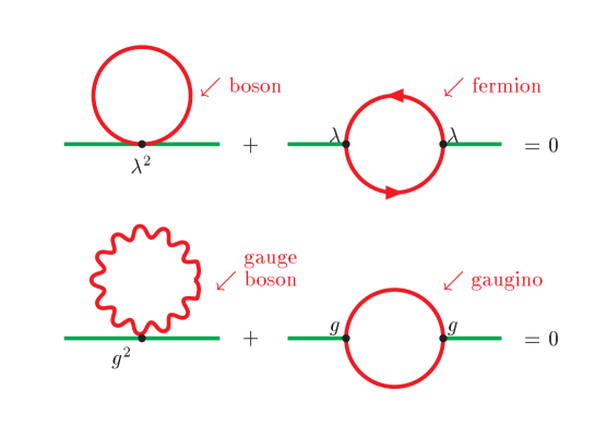
Figure 3.1: Cancellation of quadratic divergences (from reference [26])

The only known way to cancel these divergencies is supersymmetry. SUSY automatically cancels quadratic corrections to all orders of perturbation theory. This is due to the contributions of superpartners of ordinary particles. The contribution from boson loops cancel those from the fermion ones because of an additional factor (-1) coming from Fermi statistics.

The first line of Figure 3.1 shows the contribution of an SM fermion and its superpartner. The strength of interaction is given by the Yukawa coupling $\lambda$. The second line represents the gauge interaction proportional to the gauge coupling constant $g$ with the contribution from the gauge boson and its superpartner.

In both cases, cancellation of quadratic terms takes place. This cancellation occurs up to the SUSY breaking scale, $\Lambda_{SUSY}$, since

$$\sum_{bosons}m^{2}-\sum_{fermions}m^{2}=\Lambda_{SUSY}^{2}$$ (3.5)

which should be around $\sim$ 1 TeV to make the fine-tuning natural. Indeed, let us take the Higgs boson mass. Requiring for consistency of perturbation theory that the radiative corrections to the Higgs boson mass do not exceed the mass itself gives

$$\delta M_{h}^{2}\sim\frac{3y_{t}^{2}}{16\pi^{2}}\Lambda^{2}_{SUSY}\sim M_{h}^{2}$$ (3.6)

So, if $M_{h}\sim 10^{2}$ GeV one needs $\Lambda_{SUSY}\sim 10^{3}$ GeV in order that the relation (3.6) is valid. Thus, we again get more or less the same rough estimate of $\Lambda_{SUSY}\sim$ 1 TeV as from the gauge coupling unification. Two requirements match together. However as we mentioned before, $\Lambda_{SUSY}$ could be in the range $1-10$ TeV if we accept some fine-tuning.

3.1 Particles and their Superpartners

In the MSSM, we add a superpartner for each SM particle in the same representation of the gauge group. Usually we use the SUSY operators in the left-chiral representation, therefore it is convenient to rewrite the SM particles (Table 1.) in the left-chiral representation and define the superpartners accordingly. This leads to the superfield formalism, which makes it easier to construct SUSY invariant lagrangians. In this case we have to introduce for each SM particle one superfield, which contains the SM particle, its superpartner and an auxiliary unphysical field. In Table 3 we show the third generation of the SM particles, their superpartners and the superfields needed to write our lagrangian. Note that we have an extended Higgs sector and the color index is omitted.
In Table 2 we show the names of the superpartners.
Table  2.  Names  of  superpartners.Matter  Fermions⇔Sfermions(quarks, leptons)(squarks, sleptons)s=1/2s=0Gauge  Bosons⇔Gauginos(W^±, Z, γ, gluons)(Wino, Zino, photino, gluinos)s=1s=1/2Higgs⇔Higgsinoss=0s=1/2
For example the superpartner of the top quark is called stop, of the photon the superpartner is the photino, and similarly for the other particles. However, in the Higgs sector we must add another new Higgs boson and its superpartner to write the Yukawa interactions needed to generate masses for all quarks and to obtain an anomaly free model.

3.2 MSSM Lagrangian

We can divide the lagrangian of the minimal extension of the Standard Model into two fundamental parts, the SUSY invariant and the Soft breaking term [27]:

$${\cal L}_{MSSM}={\cal L}_{SUSY}+{\cal L}_{Soft}$$ (3.7)

In general we can write the SUSY invariant term as:

$${\cal L}_{SUSY}={\cal L}_{gauge}+{\cal L}_{leptons}+{\cal L}_{quarks}+{\cal L}_{Higgs}+\int{d^{2}\theta}\ {\cal W}+h.c$$ (3.8)

Defining the content of the MSSM in Table 3, we can write the different terms of the lagrangian. The term ${\cal L}_{gauge}$ has the following form:

$${\cal L}_{gauge}=\frac{1}{4}\int{d^{2}\theta}[2\ Tr(W^{3}W^{3})+2\ Tr(W^{2}W^{2})+W^{1}W^{1}]$$ (3.9)

with:

$$W^{3}_{\alpha}=-\frac{1}{4}\overline{D}\ \overline{D}\exp(-G_{3})\ D_{\alpha}\exp(G_{3})$$ (3.10)

$$G_{3}=\sum_{a=1}^{8}\frac{\lambda^{a}}{2}G^{a}_{3}\\$$ (3.11)

$$W^{2}_{\alpha}=-\frac{1}{4}\overline{D}\ \overline{D}\exp(-G_{2})\ D_{\alpha}\exp(G_{2})$$ (3.12)

$$G_{2}=\sum_{b=1}^{3}\frac{\sigma^{a}}{2}G^{b}_{2}$$ (3.13)

Table  3. Content  of  the  MSSM.SuperfieldsVector  SuperfieldsBosonic  FieldsFermionic  FieldsG_SMG^a_3G^a_μ with  a=1,2..8~G^a(8_C,1_L,0)G^b_2W^b_μ with  b=1,2,3~W^b(1_C,3_L,0)G_1B_μ~B(1_C,1_L,0)Chiral  SuperfieldsLeptonsL=(N E)~L= (~ν~e)(νe)(1_C,2_L,-1)E^C~e^Ce^C(1_C,1_L,2)QuarksQ=(U D)~Q= (~u~d)(u d)(3_C,2_L,1/3)U^C~u^Cu^C(¯3_C,1_L,-4/3)D^C~d^Cd^C(¯3_C,1_L,2/3)Higgs¯HH_1 = (H01H-1)(~H01~H-1)(1_C,2_L,-1)HH_2 = (H+2H02)(~H+2~H02)(1_C,2_L,1)

and

$$W^{1}_{\alpha}=-\frac{1}{4}\overline{D}\ \overline{D}D_{\alpha}G_{1}$$ (3.14)

where $\lambda^{a}$  and   $\sigma^{a}$  are the Gell-Mann and Pauli matrices respectively, and $G$’s are defined in Table 3.

The SUSY covariant derivatives D and $\overline{D}$ are used in the left chiral representation:

$$D_{L}=\frac{\partial}{\partial\theta}+2i\sigma^{\mu}\overline{\theta}\partial_{\mu}$$ (3.15)

and

$$\overline{D}_{L}=-\frac{\partial}{\partial\overline{\theta}}$$ (3.16)

The lagrangians for gauge interactions of leptons, quarks and the Higgs bosons are:

$${\cal L}_{leptons}=\int{d^{2}\theta\ d^{2}\overline{\theta}}\ L^{\dagger}\ \exp(2g_{2}G_{2}+g_{1}\frac{Y_{L}}{2}G_{1})\ L\ +$$

$$+\int{d^{2}\theta\ d^{2}\overline{\theta}}\ {E^{C}}^{\dagger}\ \exp(2g_{2}G_{2}+g_{1}\frac{Y_{E^{C}}}{2}G_{1})\ E^{C}$$ (3.17)

$${\cal L}_{quarks}=\int{d^{2}\theta d^{2}\ \overline{\theta}}\ Q^{\dagger}\ \exp(2g_{3}G_{3}+2g_{2}G_{2}+g_{1}\frac{Y_{Q}}{2}G_{1})\ Q\ +$$

$$+\int{d^{2}\theta\ d^{2}\overline{\theta}}\ {U^{C}}^{\dagger}\ \exp(g_{1}\frac{Y_{U^{C}}}{2}G_{1}-g_{3}(\lambda^{a})^{*}G^{a}_{3})\ U^{C}\ +$$

$$+\int{d^{2}\theta\ d^{2}\overline{\theta}}\ {D^{C}}^{\dagger}\ \exp(g_{1}\frac{Y_{D^{C}}}{2}G_{1}-g_{3}(\lambda^{a})^{*}G^{a}_{3})\ D^{C}$$ (3.18)

$${\cal L}_{Higgs}=\int{d^{2}\theta\ d^{2}\overline{\theta}}\ H^{\dagger}\ \exp(2g_{2}G_{2}+g_{1}\frac{Y_{H}}{2}G_{1})\ H\ +$$

$$+\int{d^{2}\theta\ d^{2}\overline{\theta}}\ \bar{H}^{\dagger}\ \exp(2g_{2}G_{2}+g_{1}\frac{Y_{\bar{H}}}{2}G_{1})\ \bar{H}$$ (3.19)

where $g_{3},g_{2},g_{1}$ are the SU(3), SU(2) and U(1) coupling constants, respectively. The $Y_{i}$ represent the hypercharges of the different superfields.

We can write the superpotential as the sum of two terms, $\mathcal{W}$=${\mathcal{W}}_{R}$+${\mathcal{W}}_{NR}$. The first conserves lepton (L) and baryon (B) numbers:

$${\cal W}_{R}=\epsilon_{ij}[-\mu\bar{H}^{i}H^{j}\ +\ \bar{H}^{i}L^{j}Y_{E}E^{C}\ +\ \bar{H}^{i}Q^{j}Y_{D}D^{C}\ +\ H^{j}Q^{i}Y_{U}U^{C}]$$ (3.20)

where $\epsilon_{ij}$ is the antisymmetric tensor, $\mu$ the Higgs mass parameter and $Y_{U}$, $Y_{D}$ and $Y_{E}$ are the different Yukawa matrices. The term ${\mathcal{W}}_{NR}$, which explicitly breaks L and B numbers, is:

$${\cal W}_{NR}=\epsilon_{ij}[-\mu^{{}^{\prime}}H^{i}L^{j}\ +\ \lambda L^{i}L^{j}E^{C}\ +\ \lambda^{{}^{\prime}}L^{i}Q^{j}D^{C}]\ +\ \lambda^{{}^{\prime\prime}}D^{C}D^{C}U^{C}$$ (3.21)

In ${\cal W}_{NR}$ the first three terms break lepton number, while the last term breaks baryon number. From these terms we find $d=4$ operators contributing to the decay of the proton, which will be analyzed in the next chapters. In the last section of this chapter we will analyze the R-symmetry related with the L and B number conservation and its implications.

SUSY is broken explicitly if we introduce the following terms:

$$-{\cal L}_{soft}=m^{2}_{1}|H_{1}|^{2}\ +\ m^{2}_{2}|H_{2}|^{2}\ +\ m^{2}_{12}(H_{1}H_{2}+H^{*}_{1}H^{*}_{2})$$

$$\ +\ \widetilde{Q}^{\dagger}M^{2}_{\widetilde{Q}}\widetilde{Q}\ +\ {\widetilde{u^{C}}}^{\dagger}m^{2}_{\widetilde{u}^{C}}\widetilde{u}^{C}\ +\ {\widetilde{d^{C}}}^{\dagger}m^{2}_{\widetilde{d}^{C}}{\widetilde{d}^{C}}\ +\ {\widetilde{L}}^{\dagger}M^{2}_{\widetilde{L}}\widetilde{L}\ +\ {\widetilde{E^{C}}}^{\dagger}m^{2}_{\widetilde{E}^{C}}\widetilde{E}^{C}$$

$$\ +\ [H_{2}\widetilde{Q}(Y_{U}A_{U})\widetilde{u}^{C}\ +\ H_{1}\widetilde{Q}(Y_{D}A_{D})\widetilde{d}^{C}\ +\ H_{1}\widetilde{L}(Y_{E}A_{E})\widetilde{E}^{C}+h.c]$$

$$\ +\ \frac{1}{2}[M_{1}\overline{\widetilde{B}}\widetilde{B}\ +\ M_{2}\overline{\widetilde{W^{b}}}\widetilde{W^{b}}\ +\ M_{3}\overline{\widetilde{g^{a}}}\widetilde{g^{a}}]$$ (3.22)

Note that in order to describe SUSY breaking we introduce many free parameters, and several terms have mass dimension less than 4 (super-renormalizable, but not SUSY invariant). The different mass terms remove the degeneracy between particles and their superpartners.

3.3 Neutralinos and Charginos

Once $SU(2)_{L}\times U(1)_{Y}$ is broken in the MSSM, fields with different $SU(2)_{L}\times U(1)_{Y}$ quantum numbers can mix, if they have the same $SU(3)_{C}\times U(1)_{em}$ quantum numbers, and the same spin.

The neutralinos are mixtures of the $\widetilde{B}$, the neutral $\widetilde{W}_{3}$ and the two neutral Higgsinos.

The mass term for the neutralinos is equal to:

$$-{\cal L}^{mass}_{\psi^{0}}=\frac{1}{2}(\psi^{0})^{T}\ {\cal M}_{N}\ \psi^{0}+h.c$$ (3.23)

If we define the physical states as $\widetilde{\chi^{0}_{i}}$ = $N_{ij}\psi^{0}_{j}$, the diagonal mass matrix is ${\cal M}_{D}$ = $N^{*}{\cal M}_{N}N^{\dagger}$.

In general these states form four distinct Majorana fermions, which are eigenstates of the symmetric mass matrix [in the basis ($\widetilde{B}$, $\widetilde{W_{3}}$, $\widetilde{H^{0}_{1}}$, $\widetilde{H^{0}_{2}}$)] [27]:

$${\cal M}_{N}=\left[\begin{array}[]{cccc}M_{1}&0&-m_{Z}s_{W}c_{\beta}&m_{Z}s_{W}s_{\beta}\\ 0&M_{2}&m_{Z}c_{W}c_{\beta}&-m_{Z}c_{W}s_{\beta}\\ -m_{Z}s_{W}c_{\beta}&m_{Z}c_{W}c_{\beta}&0&-\mu\\ m_{Z}s_{W}s_{\beta}&-m_{Z}c_{W}s_{\beta}&-\mu&0\end{array}\right]$$ (3.28)

where $M_{1}$ and $M_{2}$ are the SUSY breaking masses for the U(1)_Y and SU(2)_L gauginos, $\mu$ is the higgsino mass parameter, and $s_{\beta}\equiv\sin\beta$, $s_{W}\equiv\sin\theta_{W}$, etc.

We will assume that all soft breaking parameters as well as $\mu$ are real, i.e. conserve CP. We can then work with a real, orthogonal neutralino mixing matrix $N$ if we allow the eigenvalues $m_{\tilde{\chi}_{i}^{0}}$ to be negative.

This matrix can be diagonalized analytically, but the expressions of the neutralino masses and the $N_{ij}$ matrix elements are rather involved. However, if the entries in the off–diagonal $2\times 2$ submatrices are small compared to the diagonal entries, one can expand the eigenvalues in powers of $m_{Z}$ [28]:

$$m_{\tilde{\chi}_{1}^{0}} \simeq M_{1}-\frac{m_{Z}^{2}}{\mu^{2}-M_{1}^{2}}\left(M_{1}+\mu s_{2\beta}\right)s_{W}^{2}$$ (3.29)

$$m_{\tilde{\chi}_{2}^{0}} \simeq M_{2}-\frac{m_{Z}^{2}}{\mu^{2}-M_{2}^{2}}\left(M_{2}+\mu s_{2\beta}\right)c_{W}^{2}$$ (3.30)

$$m_{\tilde{\chi}_{3}^{0}} \simeq -\mu-\frac{m_{Z}^{2}(1-s_{2\beta})}{2}\left(\frac{s_{W}^{2}}{\mu+M_{1}}+\frac{c_{W}^{2}}{\mu+M_{2}}\right)$$ (3.31)

$$m_{\tilde{\chi}_{4}^{0}} \simeq \mu+\frac{m_{Z}^{2}(1+s_{2\beta})}{2}\left(\frac{s_{W}^{2}}{\mu-M_{1}}+\frac{c_{W}^{2}}{\mu-M_{2}}\right)$$ (3.32)

In our analysis, we are interested in the situation $|\mu|>M_{1},\ M_{2}$ and $\mu^{2}\gg m_{Z}^{2}$. In this case the lighter of the two neutralinos will be gaugino–like. If $|M_{1}|<|M_{2}|$, the lightest state will be bino–like, and the next–to–lightest state will be wino–like. The two heaviest states will be dominated by their higgsino components. The components of the mass eigenvectors can also be expanded in powers of $m_{Z}$. We find for the bino–like state:

$$N_{11} = \left[1+\left(N_{12}/N_{11}\right)^{2}+\left(N_{13}/N_{11}\right)^{2}+\left(N_{14}/N_{11}\right)^{2}\right]^{-1/2}$$ (3.33)

$$\frac{N_{12}}{N_{11}} = \frac{m_{Z}^{2}s_{W}c_{W}}{\mu^{2}-M_{1}^{2}}\frac{(s_{2\beta}\mu+M_{1})}{(M_{1}-M_{2})}+{\cal O}(m_{Z}^{3})$$ (3.34)

$$\frac{N_{13}}{N_{11}} = m_{Z}s_{W}\frac{(s_{\beta}\mu+c_{\beta}M_{1})}{\mu^{2}-M_{1}^{2}}+{\cal O}(m_{Z}^{2})$$ (3.35)

$$\frac{N_{14}}{N_{11}} = -m_{Z}s_{W}\frac{(c_{\beta}\mu+s_{\beta}M_{1})}{\mu^{2}-M_{1}^{2}}+{\cal O}(m_{Z}^{2})$$ (3.36)

The corresponding expressions for the wino–like state read:

$$N_{22} = \left[1+\left(N_{21}/N_{22}\right)^{2}+\left(N_{23}/N_{22}\right)^{2}+\left(N_{24}/N_{22}\right)^{2}\right]^{-1/2}$$ (3.37)

$$\frac{N_{21}}{N_{22}} = \frac{m_{Z}^{2}s_{W}c_{W}}{\mu^{2}-M_{2}^{2}}\frac{(s_{2\beta}\mu+M_{2})}{(M_{2}-M_{1})}+{\cal O}(m_{Z}^{3})$$ (3.38)

$$\frac{N_{23}}{N_{22}} = -m_{Z}c_{W}\frac{(s_{\beta}\mu+c_{\beta}M_{2})}{\mu^{2}-M_{2}^{2}}+{\cal O}(m_{Z}^{2})$$ (3.39)

$$\frac{N_{24}}{N_{22}} = m_{Z}c_{W}\frac{(c_{\beta}\mu+s_{\beta}M_{2})}{\mu^{2}-M_{2}^{2}}+{\cal O}(m_{Z}^{2})$$ (3.40)

Note that the higgsino components of the gaugino–like states start at ${\cal O}(m_{Z})$, whereas the masses of these states deviate from their $|\mu|\rightarrow\infty$ limit ($M_{1}$ and $M_{2}$) only at ${\cal O}(m_{Z}^{2})$.

The charginos are mixtures of the $\widetilde{W}^{\pm}$ and $\widetilde{H}^{\pm}$. The chargino mass matrix [in the basis ($\widetilde{W^{\pm}},\widetilde{H^{\pm}}$) ] [27]is:

$${\cal M}_{C}=\left[\begin{array}[]{cc}M_{2}&\sqrt{2}m_{W}s_{\beta}\\ \sqrt{2}m_{W}c_{\beta}&\mu\end{array}\right]$$ (3.43)

if we expand in powers of $m_{W}$, the two chargino masses are:

$$m_{\tilde{\chi}_{1}^{\pm}}\simeq M_{2}-\frac{m_{W}^{2}}{\mu^{2}-M_{2}^{2}}\left(M_{2}+\mu s_{2\beta}\right)\simeq m_{\tilde{\chi}_{2}^{0}}\ \ \ \$$ (3.44)

$$m_{\tilde{\chi}_{2}^{\pm}}\simeq\mu+\frac{m_{W}^{2}}{\mu^{2}-M_{2}^{2}}\left(M_{2}s_{2\beta}+\mu\right)$$ (3.45)

so that for $|\mu|\rightarrow\infty$, the lightest chargino corresponds to a pure wino state while the heavier chargino corresponds to a pure higgsino state.

Usually the neutralino is considered the lightest supersymmetric particle (LSP) in models where R-parity is conserved. It has been realized many years ago that they are good candidates to describe the Non-Baryonic Dark Matter present in the Universe [7, 8, 9]. There is no direct experimental limit for the neutralino mass, however from LEP experiments we know that the chargino mass $m_{\tilde{\chi_{1}^{\pm}}}$ must be bigger than $103.5$ GeV[29].

3.4 Squarks and Sleptons

After the electroweak symmetry breaking, several terms in the MSSM lagrangian contribute to the sfermion mass matrices. Ignoring flavor mixing between sfermions, the mass matrix for charged matter sfermion is[in the basis $(\tilde{f},\tilde{f}^{C})$] [27]:

$${\cal M}^{2}_{\tilde{f}}=\left(\begin{array}[]{cc}m_{f}^{2}+m_{LL}^{2}&m_{f}\,\tilde{A}_{f}\\ m_{f}\,\tilde{A}_{f}&m_{f}^{2}+m_{RR}^{2}\end{array}\right)$$ (3.48)

with

$$\begin{array}[]{l}\ m_{LL}^{2}=m_{\tilde{f}}^{2}+(I_{3}^{f}-Q_{f}\sin^{2}\theta_{W})\,m_{Z}^{2}\,\cos 2\beta\\ \\ m_{RR}^{2}=m_{\tilde{f}^{C}}^{2}+Q_{f}\sin^{2}\theta_{W}\,m_{Z}^{2}\,\cos 2\beta\\ \\ \ \tilde{A}_{f}=A_{f}-\mu(\tan\beta)^{-2I_{3}^{f}}\end{array}$$ (3.54)

where $f$ represents the different charged fermions $u^{i}$, $d^{i}$ and $e^{i}$.

The charged sfermions mass matrices are diagonalized by $2\times 2$ rotation matrices described by the angles $\theta_{\tilde{f}}$, which turn the current eigenstates, $\tilde{f}$ and $\tilde{f}^{C}$, into the mass eigenstates $\tilde{f}_{1}$ and $\tilde{f}_{2}$; the mixing angle and sfermion masses are then given by

$$\sin 2\theta_{\tilde{f}}=\frac{2m_{f}\tilde{A}_{f}}{m_{\tilde{f}_{1}}^{2}-m_{\tilde{f}_{2}}^{2}}\ \ ,\ \ \cos 2\theta_{\tilde{f}}=\frac{m_{LL}^{2}-m_{RR}^{2}}{m_{\tilde{f}_{1}}^{2}-m_{\tilde{f}_{2}}^{2}},\hskip 22.76228pt$$ (3.55)

$$m_{\tilde{f}_{1,2}}^{2}=m_{f}^{2}+\frac{1}{2}\left[m_{LL}^{2}+m_{RR}^{2}\mp\sqrt{(m_{LL}^{2}-m_{RR}^{2})^{2}+4m_{f}^{2}\tilde{A}_{f}^{2}}\ \right]$$ (3.56)

The physical states are defined as:

$$\widetilde{f}_{1}=\widetilde{f}\cos\theta_{\widetilde{f}}+\widetilde{f}^{C}\sin\theta_{\widetilde{f}}$$ (3.57)

and

$$\widetilde{f}_{2}=-\widetilde{f}\sin\theta_{\widetilde{f}}+\widetilde{f}^{C}\cos\theta_{\widetilde{f}}$$ (3.58)

In the case of sneutrinos we have:

$${\cal M}^{2}_{\tilde{\nu}}=M^{2}_{\tilde{L}}+\frac{1}{2}m^{2}_{Z}\cos 2\beta$$ (3.59)

Note the contributions of the different soft breaking parameters in the mass matrices.

3.5 Higgs Bosons

As we have mentioned before, the existence of a scalar Higgs boson is the main motivation to introduce SUSY. In the MSSM the tree-level Higgs potential is given by [27][30]:

$$V_{Higgs}=m^{2}_{H_{1}}|H_{1}|^{2}+m^{2}_{H_{2}}|H_{2}|^{2}+m^{2}_{12}(H_{1}H_{2}+h.c)+$$ (3.60)

$$+\frac{g^{2}_{1}+g^{2}_{2}}{8}(|H_{1}|^{2}-|H_{2}|^{2})^{2}+\frac{g^{2}_{2}}{2}|H^{\dagger}_{1}H_{2}|^{2}$$ (3.61)

where $m^{2}_{H_{i}}=m^{2}_{i}+|\mu|^{2}$ with $i=1,2$

Note that in this equation the strength of the quartic interactions is determined by the gauge couplings.

After electroweak symmetry breaking, three of the eight degrees of freedom contained in the two Higgs boson doublets get eaten by the $W^{\pm}$ and $Z$ gauge bosons. The five physical degrees of freedom that remain form a neutral pseudoscalar boson $A^{0}$, two neutral scalar Higgs bosons $h^{0}$ and $H^{0}$, and two charged Higgs bosons $H^{+}$ and $H^{-}$.

The physical pseudoscalar Higgs boson $A^{0}$ is a linear combination of the imaginary parts of $H^{0}_{1}$ and $H^{0}_{2}$, which have the mass matrix [ in the basis $(\frac{Im\ H^{0}_{1}}{\sqrt{2}},\frac{Im\ H^{0}_{2}}{\sqrt{2}})$]:

$$\small{M^{2}_{I}=\left(\begin{array}[]{cc}-m^{2}_{12}\ \tan\beta&-m^{2}_{12}\\ -m^{2}_{12}&-m^{2}_{12}\ \cot\beta\end{array}\right)}$$ (3.62)

$$m^{2}_{A^{0}}=trM^{2}_{I}=-2m^{2}_{12}\ /\sin(2\beta)$$ (3.63)

The other neutral Higgs bosons are mixtures of the real parts of $H^{0}_{1}$ and $H^{0}_{2}$, with tree-level mass matrix [$\frac{Re\ H^{0}_{1}}{\sqrt{2}},\frac{Re\ H^{0}_{2}}{\sqrt{2}}$]:

$$\small{M^{2}_{R}=\left(\begin{array}[]{cc}-m^{2}_{12}\tan\beta+m^{2}_{Z}\cos^{2}\beta&m^{2}_{12}-\frac{1}{2}m^{2}_{Z}\sin 2\beta\\ m^{2}_{12}-\frac{1}{2}m^{2}_{Z}\sin 2\beta&-m^{2}_{12}\cot\beta+m^{2}_{Z}\sin^{2}\beta\end{array}\right)}$$ (3.64)

In this case the eigenvalues are:

$$m^{2}_{H^{0},h^{0}}=\frac{1}{2}[m^{2}_{A^{0}}+m^{2}_{Z}\pm\sqrt{(m^{2}_{A^{0}}+m^{2}_{Z})^{2}-4m^{2}_{A^{0}}m^{2}_{Z}\cos^{2}(2\beta)}]$$ (3.65)

Explicitly the mass eigenstates are:

$$\begin{array}[]{l}\left\{\begin{array}[]{lllr}G^{0}&=&\frac{1}{\sqrt{2}}[-\cos\beta\ Im\ H^{0}_{1}+\sin\beta\ Im\ H^{0}_{2}],&\ \ \ Goldstone\ boson\to Z^{0},\\ A^{0}&=&\frac{1}{\sqrt{2}}[\sin\beta\ Im\ H^{0}_{1}+\cos\beta\ Im\ H^{0}_{2}],&\ \ \ \ \ \ \ \ Pseudoscalar\ Higgs,\end{array}\right.\\ \\ \left\{\begin{array}[]{lllr}G^{+}&=&\frac{1}{\sqrt{2}}[-\cos\beta\ (H^{-}_{1})^{*}+\sin\beta\ H^{+}_{2}],&\ \ \ \ \ \ \ Goldstone\ boson\to W^{+},\\ H^{+}&=&\frac{1}{\sqrt{2}}[\sin\beta\ (H^{-}_{1})^{*}+\cos\beta\ H^{+}_{2}],&\ \ \ Charged\ Higgs,\end{array}\right.\\ \\ \left\{\begin{array}[]{lllr}h^{0}&=&\frac{1}{\sqrt{2}}[-\sin\alpha\ Re\ H^{0}_{1}+\cos\alpha\ Re\ H^{0}_{2}],&\ \ \ \ \ \ \ light\ Higgs,\\ H^{0}&=&\frac{1}{\sqrt{2}}[\cos\alpha\ Re\ H^{0}_{1}+\sin\alpha\ Re\ H^{0}_{2}],&\ \ \ \ \ \ \ heavy\ Higgs,\end{array}\right.\end{array}$$

where the mixing angle $\alpha$ is given by:

$$\tan 2\alpha=-\tan 2\beta\left(\frac{m^{2}_{A^{0}}+M^{2}_{Z}}{m^{2}_{A^{0}}-M^{2}_{Z}}\right)$$ (3.66)

From these equations we can see that at tree level, the MSSM predict that $m_{h^{0}}\leq m_{Z}$, however when we consider one-loop corrections, the mass of the light Higgs boson is modified significantly. For example assuming that the stop masses do not exceed 1 TeV, $m_{h^{0}}\raisebox{-3.69899pt}{~{}\shortstack{$<$ \\ [-0.07cm] $\sim$}}~{}130\ \rm{GeV}$ [31].

3.6 The R-symmetry and its Implications

In the Standard Model the conservation of Baryon (B) and Lepton (L) number is automatic, this is an accidental consequence of the gauge group and matter content. In the MSSM, as we showed in the second section of this chapter, we can separate the most general gauge invariant superpotential into two fundamental parts, where the first term conserves B and L, while the second breaks these symmetries.

In the MSSM, B and L conservation can be related to a new discrete symmetry, which can be used to classify the two kinds of contributions to the superpotential. This symmetry is the matter-parity, defined as:

$$M=(-1)^{3(B-L)}$$ (3.67)

Quark and lepton supermultiplets have $M=-1$, while the Higgs and gauge supermultiplets have $M=+1$. The symmetry principle in this case will be that a term in the lagrangian is allowed only if the product of the M parities is equal to 1.

The conservation of matter-parity as defined in equation (3.67), together with spin conservation, also implies the conservation of another discrete symmetry called R-parity, defined such that it will be +1 for the SM particles and -1 for all the sparticles:

$$R=(-1)^{2S}M$$ (3.68)

These two symmetries are equivalent, since in the superpotential only the scalar fields get v.e.v. However only M commutes with the SUSY generators.

Now if we impose the conservation of $R$, we will have some important phenomenological consequences in SUSY models:

• The lightest particle with $R=-1$, called the lightest supersymmetric particle (LSP), must be stable.

• Each sparticle other than the LSP must decay into a state with an odd number of LSPs.

• Sparticles can only be produced in even numbers from SM particles.

• There are not $d=4$ operators contributing to the decay of the proton.

It is important to mention that the conservation of $R$ parity is predicted in a large class of Supersymmetric Grand Unified Theories as Minimal SUSY $SO(10)$[32, 33].

Chapter 4 SUSY decays of neutral Higgs bosons

In this chapter we will analyze different aspects related to supersymmetric decays of the Higgs bosons in the Minimal Supersymmetric Standard Model (MSSM), studying the Higgs decays into two neutralinos. In particular we will compute and show the effect of new loop corrections to the Higgs-neutralino-neutralino couplings and to the invisible branching ratios.

4.1 Higgs decays in the MSSM

In order to provide a complete analysis of the most important aspects of Higgs decays in the Minimal Supersymmetric Standard Model (MSSM), we will start with the properties of the SM Higgs boson. The Higgs mass $m^{2}_{h_{SM}}=\frac{1}{2}\lambda v^{2}$ is a free parameter, since $\lambda$ is unknown at present. However the theory predicts the Higgs couplings to fermions and gauge bosons as:

$$g^{SM}_{hf\bar{f}}=\frac{m_{f}}{v}\qquad\qquad g^{SM}_{hVV}=\frac{2m^{2}_{V}}{v}$$ (4.1)

where $f$ is used for any fermion, and $V$ for $W^{\pm}$ and $Z^{0}$. In Fig 4.1 the different SM Higgs branching ratios versus $m_{h_{SM}}$ is plotted.

Figure 4.1: The decay branching ratios (left) and the total decay width (right) of the SM Higgs boson as a function of its mass.[from reference [34]]

From this figure we can appreciate that there are two important intervals, for $m_{h_{SM}}\raisebox{-3.69899pt}{~{}\shortstack{$<$ \\ [-0.07cm] $\sim$}}~{}135\ GeV$ the most important channel is $h_{SM}\to b\ \bar{b}$ with branching ratio close to $\sim 90\%$, while for $m_{h_{SM}}\raisebox{-3.69899pt}{~{}\shortstack{$>$ \\ [-0.07cm] $\sim$}}~{}135\ GeV$ the dominant decay mode is $h_{SM}\to W\ W^{*}$ (where one of the gauge bosons may be virtual). This behaviour is easy to understand if we take a look at the couplings listed above. There are other important channels such as $h_{SM}\to\tau^{+}\ \tau^{-}$, $h_{SM}\to c\ \bar{c}$, and at one-loop we have the decays $h_{SM}\to g\ g$ and $h_{SM}\to\gamma\ \gamma$, which are important for Higgs searches [31]. In the low mass range, the Higgs width is very narrow, with $\Gamma<10\ MeV$, but increasing $m_{h_{SM}}$ we reach $1\ GeV$ at the $Z^{0}\ Z^{0}$ threshold (see Fig 4.1).

The same analysis in the context of the MSSM is more difficult, due to the presence of three neutral Higgs bosons and one charged pair. There are new decay modes which modify the branching ratios of all the channels, in particular the decay into supersymmetric particles could play an important role [35, 36, 37, 38].

In order to understand how the branching ratio are modified, we list the couplings of the neutral Higgs bosons to $f\ \bar{f}$ relative to the Standard Model values:


for the light CP-even Higgs $h^{0}$:

$$h^{0}\ d_{i}\ \bar{d_{i}}(\ or\ e_{i}\ \bar{e_{i}}\ ):-\frac{\sin\alpha}{\cos\beta}\qquad\qquad h^{0}\ u_{i}\ \bar{u_{i}}:\frac{\cos\alpha}{\sin\beta}$$ (4.2)

for the heavy CP-even $H^{0}$

$$H^{0}\ d_{i}\ \bar{d_{i}}(\ or\ e_{i}\ \bar{e_{i}}\ ):\frac{\cos\alpha}{\cos\beta}\qquad\qquad H^{0}\ u_{i}\ \bar{u_{i}}:\frac{\sin\alpha}{\sin\beta}$$ (4.3)

and for the CP-odd $A^{0}$ we have:

$$A^{0}\ d_{i}\ \bar{d_{i}}(\ or\ e_{i}\ \bar{e_{i}}\ ):\gamma_{5}\tan\beta\qquad\qquad A^{0}\ u_{i}\ \bar{u_{i}}:\gamma_{5}\cot\beta$$ (4.4)

Figure 4.2: Dominant MSSM Higgs bosons decay branching ratios as functions of the Higgs boson masses for $\tan\beta=3$ and 30.[from reference [34]]

while the couplings of the two CP-even Higgs bosons to $W^{\pm}$ and $Z^{0}$ pairs are given by:

$$g_{h^{0}VV}=g^{SM}_{h^{0}VV}\sin(\beta-\alpha)\qquad\qquad g_{H^{0}VV}=g^{SM}_{H^{0}VV}\cos(\beta-\alpha)$$ (4.5)

From the couplings listed above, we note that there are two new parameters which will play an important role in the prediction of the branching ratios of neutral Higgs bosons. For example the decay mode $h^{0}\to b\ \bar{b}$ could be significantly modified at large values of $\tan\beta$ and/or small values of $\sin\alpha$. The prediction of the branching ratios depends on the set of MSSM parameters, in particular the spectrum of SUSY particles change appreciably the SUSY Higgs decays.

In Fig 4.2 we show the different decay modes of the neutral Higgs bosons for two different values of $\tan\beta$ as functions of the Higgs masses. The branching ratio of the charged Higgs boson is also shown in order to complete our analysis. As we know there is a limit for the light Higgs mass in the MSSM, $m_{h^{0}}\raisebox{-3.69899pt}{~{}\shortstack{$<$ \\ [-0.07cm] $\sim$}}~{}130\ GeV$[31], therefore $h^{0}$ will decay mainly into fermion pairs, in particular the most important channel is $h^{0}\to b\ \bar{b}$. This is in general also the dominant decay mode of the $H^{0}$ and $A^{0}$ bosons, since for $\tan\beta\gg 1$ the decay rate into $b\bar{b}$ and $\tau^{-}\tau^{+}$ pairs are of the order of $90\%$ and $10\%$, respectively. For large masses the top decay channels $H^{0},A^{0}\to t\ \bar{t}$ are suppressed for large $\tan\beta$.

In order to complete our analysis, the SUSY decays of the neutral Higgs bosons must be considered, which could be dominant in different regions of the parameter space. In general any Higgs boson could decay into sfermions (squarks and sleptons), charginos or neutralinos. However taking into account the lastest results of the SUSY searches experiments [29], we know that in the case of the light Higgs boson, the only allowed SUSY channels are two neutralinos or two sneutrinos. For the heavy CP-even and CP-odd Higgs bosons the decays into squarks or charginos are also allowed, excluding the decay of $A^{0}$ into two sneutrinos.

These SUSY decays will be dominant, of course, when the channels present in the Standard Model are suppressed. As we already noted the most important decay models are the decays into $b$ or $\tau$ pairs, these channels are suppressed in the case of low or moderate $\tan\beta$, or when the mixing angle $\alpha$ of the Higgs sector is quite small. Combining these two scenarios, we will able to get significant branching ratios for these channels.

The various decay widths and branching ratios of the SM and MSSM can be calculated in a very precise way with the Fortran code HDECAY [39], where all the relevant experimental constraints are taken into account. The subroutines of HDECAY dealing with the decays of neutral Higgs bosons into neutralinos use the results of reference [28].

4.2 Higgs boson decays into two Neutralinos

In the Standard Model there are no invisible decays of the Higgs boson, since no $\nu_{R}$ is present in the model. In the MSSM the situation is quite different, there are new couplings which allow new decays of the Higgs bosons. The MSSM neutral Higgs bosons $h^{0},H^{0}$ and $A^{0}$ could decay into invisible neutralino $\tilde{\chi}^{0}_{1}$ or sneutrino $\tilde{\nu}$ pairs. These decay modes are invisible in the case that the neutralinos or sneutrinos are the lightest SUSY particles (LSP) and $R$-parity is conserved. Note that in the case of the CP-odd Higgs field, there is only one possibility, the decays into two neutralinos, since the coupling to two sneutrinos does not exist. In this section we will describe in detail neutral Higgs decays into two neutralinos in the gaugino limit, considering quantum corrections at one-loop level.

Before computing and discussing the partial widths for the decays of the neutral Higgs bosons into pairs of identical neutralinos, let us discuss the properties of the couplings $g^{0}_{\Phi\ \tilde{\chi}_{1}^{0}\ \tilde{\chi}_{1}^{0}}$, where $\Phi=h^{0},H^{0}$ and $A^{0}$ and $\tilde{\chi}_{1}^{0}$ is the lightest neutralino, in our case the lightest supersymmetric particle (LSP).

At tree level, the couplings of the neutralinos $\tilde{\chi}_{i}^{0}$ to the neutral CP-even Higgs bosons $\phi=h^{0},H^{0}$ and to the CP-odd boson $A^{0}$ are given by:

$$g^{0}_{\phi\tilde{\chi}_{i}^{0}\tilde{\chi}_{j}^{0}}=\frac{g}{2}\left[(N_{i2}-\tan\theta_{W}N_{i1})(d_{\phi}N_{j3}+e_{\phi}N_{j4})\ +\ i\leftrightarrow j\right]$$ (4.6)

$$g^{0}_{A^{0}\tilde{\chi}_{i}^{0}\tilde{\chi}_{j}^{0}}=\frac{g}{2}\left[(N_{i2}-\tan\theta_{W}N_{i1})(d_{A^{0}}N_{j3}+e_{A^{0}}N_{j4})\ +\ i\leftrightarrow j\right]$$ (4.7)

where the quantities $d_{\Phi}$ and $e_{\Phi}$ are:

$$d_{H^{0}}=-\cos\alpha\ ,\ d_{h^{0}}=\sin\alpha\ ,\ d_{A^{0}}=\sin\beta$$ (4.8)

$$e_{H^{0}}=\sin\alpha\ ,\ e_{h^{0}}=\cos\alpha\ ,\ e_{A^{0}}=-\cos\beta.$$ (4.9)

and $N_{ij}$ are the components of the matrix which diagonalizes the four dimensional neutralino mass matrix.

Now using these equations we find the expressions for $g^{0}_{\Phi\ \tilde{\chi}_{1}^{0}\ \tilde{\chi}_{1}^{0}}$ :

$$g^{0}_{h^{0}\tilde{\chi}_{1}^{0}\tilde{\chi}_{1}^{0}}=g\left[(N_{12}-\tan\theta_{W}N_{11})(\sin\alpha N_{13}+\cos\alpha N_{14})\right]$$ (4.10)

$$g^{0}_{H^{0}\tilde{\chi}_{1}^{0}\tilde{\chi}_{1}^{0}}=g\left[(N_{12}-\tan\theta_{W}N_{11})(-\cos\alpha N_{13}+\sin\alpha N_{14})\right]$$ (4.11)

$$\gamma_{5}\ g^{0}_{A^{0}\tilde{\chi}_{1}^{0}\tilde{\chi}_{1}^{0}}=\gamma_{5}\ g\left[(N_{12}-\tan\theta_{W}N_{11})(\sin\beta N_{13}-\cos\beta N_{14})\right]$$ (4.12)

we see that all these couplings are exactly zero in the pure gaugino $(N_{13}=N_{14}=0)$ or higgsino $(N_{11}=N_{12}=0)$ limit.

Inserting eqs. (3.33) into eqs. (4.10) to (4.12), we see that the LSP couplings to the Higgs bosons $\Phi=h^{0},H^{0},A^{0}$ already receive contributions at ${\cal O}(m_{Z})$:

$$g^{0}_{\Phi\tilde{\chi}_{1}^{0}\tilde{\chi}_{1}^{0}}\sim d_{\Phi}N_{13}+e_{\Phi}N_{14}\sim s_{W}m_{Z}\left[\frac{(d_{\Phi}s_{\beta}-e_{\Phi}c_{\beta})\mu}{\mu^{2}-M_{1}^{2}}+\frac{(d_{\Phi}c_{\beta}-e_{\Phi}s_{\beta})M_{1}}{\mu^{2}-M_{1}^{2}}\right]$$ (4.13)

Similar expressions can be given for the couplings of the wino–like state.

This suppression of the tree–level couplings follows from the fact that, in the neutralino sector, the Higgs boson couples only to one higgsino and one gaugino current eigenstate, together with the fact that mixing between current eigenstates is suppressed if $|\mu|\gg m_{Z}$. These couplings thus vanish as $|\mu|\rightarrow\infty$.

Knowing all the properties of the couplings, and taking into account that neutralinos are Majorana particles, we are able to compute the partial widths for the decays of the neutral Higgs bosons, $\Phi=h^{0},H^{0}$, and $A^{0}$, into pairs of identical neutralinos:

$$\Gamma(\Phi\rightarrow\tilde{\chi}_{1}^{0}\tilde{\chi}_{1}^{0})=\frac{\beta_{\Phi}^{n}M_{\Phi}}{16\pi}\left|g^{0}_{\Phi\tilde{\chi}_{1}^{0}\tilde{\chi}_{1}^{0}}+g^{1}_{\Phi\tilde{\chi}_{1}^{0}\tilde{\chi}_{1}^{0}}\right|^{2}.$$ (4.14)

where $n=3$ for the CP–even fields $h^{0}$ and $H^{0}$, while for the CP–odd $A^{0}$ Higgs boson $n=1$. $M_{\Phi}$ is the Higgs mass, and ${\beta_{\Phi}}^{2}=(1-\frac{4\ m^{2}_{\tilde{\chi}_{1}^{0}}}{M^{2}_{\Phi}})$. We include the possible one-loop corrections to the couplings $g^{1}_{\Phi\tilde{\chi}_{1}^{0}\tilde{\chi}_{1}^{0}}$, which will be discussed in the next section.

4.3 Higgs decays into Neutralinos at one-loop

At the one-loop level, the couplings of the lightest neutralinos to the Higgs bosons can be generated, in principle, by diagrams with the exchange of either sfermions and fermions, or of charginos or neutralinos together with gauge or Higgs bosons, in the loop. However, the latter class of diagrams can contribute to the couplings of Higgs bosons to neutralinos only if one of the particles in the loop is a higgsino. These loop contributions will thus be suppressed by inverse powers of $|\mu|$, in addition to the usual loop suppression factor, since the couplings $g^{0}(H^{\pm}\tilde{\chi}_{1}^{0}\tilde{\chi}_{1}^{\mp})\sim{\cal O}(m_{W}/\mu),\ g^{0}(W^{\pm}\tilde{\chi}_{1}^{0}\tilde{\chi}_{1}^{\mp})\sim{\cal O}(m^{2}_{W}/\mu^{2})$ in the gaugino limit. We therefore do not expect them to be able to compete with the tree–level couplings that exist for finite $|\mu|$.

We consider diagrams with fermions and sfermions in the loop, as shown below. For the $\Phi\tilde{\chi}_{1}^{0}\tilde{\chi}_{1}^{0}$ couplings, only the third generation (s)particles, which have large Yukawa couplings, can give significant contributions to the amplitudes. Note that in the bino limit there is no wave function renormalization to perform, since the tree–level couplings are zero. Off–diagonal wave function renormalization diagrams could convert one of the gaugino–like neutralinos into a higgsino–like state, but this kind of contribution is again suppressed by $1/|\mu|$, and can thus not compete with the tree–level coupling.

The Feynman diagrams contributing to the one–loop couplings of the lightest neutralinos to the $\Phi=h^{0},H^{0}$ and $A^{0}$ Higgs bosons. Diagrams with crossed neutralino lines have to be added.

We have calculated the contributions of these diagrams for arbitrary momentum square of the Higgs, finite masses for the internal fermions and sfermions as well as for the external LSP neutralinos, and taking into account the full mixing in the sfermion sector. The amplitudes are ultra–violet finite as it should be. The contributions from diagrams a) and b) to the $\Phi\tilde{\chi}_{1}^{0}\tilde{\chi}_{1}^{0}$ couplings are separately finite for each fermion species. We have performed the calculation in the dimensional reduction scheme [40, 41]; since the one–loop couplings are finite and do not require any renormalization, the result should be scheme independent. The results are given below for a general gaugino limit ($|\mu|\gg M_{1},M_{2}$, for arbitrary ordering of $M_{1}$ and $M_{2}$).

The one–loop Higgs boson couplings to the LSP neutralinos in the gaugino limit are given by:

$$g^{1}_{\phi\tilde{\chi}_{1}^{0}\tilde{\chi}_{1}^{0}}=\frac{g}{4\pi^{2}}\bigg{[}\sum_{f}N_{c}\delta_{\phi}^{(f)}\bigg{]}$$ (4.15)

$$g^{1}_{A^{0}\tilde{\chi}_{1}^{0}\tilde{\chi}_{1}^{0}}=\frac{g}{4\pi^{2}}\bigg{[}\sum_{f}N_{c}\delta_{A^{0}}^{(f)}\bigg{]}$$ (4.16)

where

$$\delta_{\phi}^{(f)} = \frac{m_{f}g_{\phi ff}}{2m_{W}}\left\{s_{2\theta_{\tilde{f}}}(v_{1}+v_{3})\left[-\left(m_{\tilde{f}_{1}}^{2}+m_{f}^{2}+m_{\tilde{\chi}_{1}^{0}}^{2}\right)C_{0}(\tilde{f}_{1})+4m_{\tilde{\chi}_{1}^{0}}^{2}C_{1}^{+}(\tilde{f}_{1})\right.\right.$$ (4.17)

$$\ \ \ +\left.\left(m_{\tilde{f}_{2}}^{2}+m_{f}^{2}+m_{\tilde{\chi}_{1}^{0}}^{2}\right)C_{0}(\tilde{f}_{2})-4m_{\tilde{\chi}_{1}^{0}}^{2}C_{1}^{+}(\tilde{f}_{2})\right]$$

$$+\ 2(v_{1}+v_{2}c^{2}_{\theta_{\tilde{f}}})m_{f}m_{\tilde{\chi}_{1}^{0}}\left[C_{0}(\tilde{f}_{1})-2C_{1}^{+}(\tilde{f}_{1})\right]$$

$$+\left.2(v_{1}+v_{2}s^{2}_{\theta_{\tilde{f}}})m_{f}m_{\tilde{\chi}_{1}^{0}}\left[C_{0}(\tilde{f}_{2})-2C_{1}^{+}(\tilde{f}_{2})\right]\right\}$$

$$- C_{\phi\tilde{f}_{1}\tilde{f}_{1}}\left\{-s_{2\theta_{\tilde{f}}}(v_{1}+v_{3})m_{f}C_{0}(\tilde{f}_{1},\tilde{f}_{1})+2(v_{1}+v_{2}c^{2}_{\theta_{\tilde{f}}})m_{\tilde{\chi}_{1}^{0}}C_{1}^{+}(\tilde{f}_{1},\tilde{f}_{1})\right\}$$

$$- C_{\phi\tilde{f}_{2}\tilde{f}_{2}}\left\{s_{2\theta_{\tilde{f}}}(v_{1}+v_{3})m_{f}C_{0}(\tilde{f}_{2},\tilde{f}_{2})+2(v_{1}+v_{2}s^{2}_{\theta_{\tilde{f}}})m_{\tilde{\chi}_{1}^{0}}C_{1}^{+}(\tilde{f}_{2},\tilde{f}_{2})\right\}$$

$$- C_{\phi\tilde{f}_{1}\tilde{f}_{2}}\left\{-2c_{2\theta_{\tilde{f}}}(v_{1}+v_{3})m_{f}C_{0}(\tilde{f}_{1},\tilde{f}_{2})-2s_{2\theta_{\tilde{f}}}v_{2}m_{\tilde{\chi}_{1}^{0}}C_{1}^{+}(\tilde{f}_{1},\tilde{f}_{2})\right\}$$

$$\delta_{A^{0}}^{(f)}=\frac{m_{f}g_{A^{0}ff}}{2m_{W}}\left\{(v_{1}+v_{3})s_{2\theta_{\tilde{f}}}\left[\left(m_{\tilde{f}_{1}}^{2}-m_{f}^{2}-m_{\tilde{\chi}_{1}^{0}}^{2}\right)C_{0}(\tilde{f}_{1})-\left(m_{\tilde{f}_{2}}^{2}-m_{f}^{2}-m_{\tilde{\chi}_{1}^{0}}^{2}\right)C_{0}(\tilde{f}_{2})\right]\right\}$$

$$+\frac{m_{f}g_{A^{0}ff}}{2m_{W}}\left\{2(v_{1}+v_{2}c^{2}_{\theta_{\tilde{f}}})m_{\tilde{\chi}_{1}^{0}}m_{f}C_{0}(\tilde{f}_{1})+2(v_{1}+v_{2}s^{2}_{\theta_{\tilde{f}}})m_{\tilde{\chi}_{1}^{0}}m_{f}C_{0}(\tilde{f}_{2})\right\}$$

$$+ C_{A^{0}\tilde{f}_{1}\tilde{f}_{2}}\left\{-2m_{f}(v_{1}+v_{3})C_{0}(\tilde{f}_{1},\tilde{f}_{2})+2m_{\tilde{\chi}_{1}^{0}}(2v_{1}+v_{2})s_{2\theta_{\tilde{f}}}C_{1}^{-}(\tilde{f}_{1},\tilde{f}_{2})\right\}$$

The Higgs–fermion–fermion coupling constants are given by

$$g_{h^{0}uu} = \frac{\cos\alpha}{\sin\beta}\qquad,\qquad g_{h^{0}dd}=-\frac{\sin\alpha}{\cos\beta}\ ,$$

$$g_{H^{0}uu} = \frac{\sin\alpha}{\sin\beta}\qquad,\qquad g_{H^{0}dd}=\frac{\cos\alpha}{\cos\beta}\ ,$$

$$g_{A^{0}uu} = \cot\beta\qquad,\qquad g_{A^{0}dd}=\tan\beta\ ,$$ (4.19)

and

$$v_{1} = \ \frac{1}{2}\left(gQ_{f}N_{11}\tan\theta_{W}\right)^{2},$$

$$v_{2} = \frac{I_{3}^{f}}{2Q_{f}}v_{0}\left[-2+\frac{I_{3}^{f}}{Q_{f}}+2\left(1-\frac{I_{3}^{f}}{Q_{f}}\right)\frac{N_{12}}{N_{11}\tan\theta_{W}}+\frac{I_{3}^{f}}{Q_{f}}\left(\frac{N_{12}}{N_{11}\tan\theta_{W}}\right)^{2}\right],$$

$$v_{3} = \frac{I_{3}^{f}}{2Q_{f}}v_{0}\left(\frac{N_{12}}{N_{11}\tan\theta_{W}}-1\right).$$ (4.20)

while the Higgs–sfermion–sfermion coupling constants read:

$$C_{h^{0}\tilde{u}_{1}\tilde{u}_{1}}=\frac{m_{Z}}{c_{W}}s_{\beta+\alpha}\left[I_{3}^{u}c^{2}_{\theta_{\tilde{u}}}-Q_{u}s^{2}_{W}c_{2\theta_{\tilde{u}}}\right]-\frac{m_{u}^{2}g_{h^{0}uu}}{m_{W}}-\frac{m_{u}s_{2\theta_{\tilde{u}}}}{2m_{W}}\left[A_{u}g_{h^{0}uu}+\mu g_{H^{0}uu}\right]$$

$$C_{h^{0}\tilde{u}_{2}\tilde{u}_{2}}=\frac{m_{Z}}{c_{W}}s_{\beta+\alpha}\left[I_{3}^{u}s^{2}_{\theta_{\tilde{u}}}+Q_{u}s^{2}_{W}c_{2\theta_{\tilde{u}}}\right]-\frac{m_{u}^{2}g_{h^{0}uu}}{m_{W}}+\frac{m_{u}s_{2\theta_{\tilde{u}}}}{2m_{W}}\left[A_{u}g_{h^{0}uu}+\mu g_{H^{0}uu}\right]$$

$$C_{h^{0}\tilde{u}_{1}\tilde{u}_{2}}=\frac{m_{Z}}{c_{W}}s_{\beta+\alpha}\left[Q_{u}s^{2}_{W}-I_{3}^{u}/2\right]s_{2\theta_{\tilde{u}}}-\frac{m_{u}}{2m_{W}}\left[A_{u}g_{h^{0}uu}+\mu g_{H^{0}uu}\right]c_{2\theta_{\tilde{u}}}$$

$$C_{h^{0}\tilde{d}_{1}\tilde{d}_{1}}=\frac{m_{Z}}{c_{W}}s_{\beta+\alpha}\left[I_{3}^{d}c^{2}_{\theta_{\tilde{d}}}-Q_{d}s^{2}_{W}c_{2\theta_{\tilde{d}}}\right]-\frac{m_{d}^{2}g_{h^{0}dd}}{m_{W}}-\frac{m_{d}s_{2\theta_{\tilde{d}}}}{2m_{W}}\left[A_{d}g_{h^{0}dd}-\mu g_{H^{0}dd}\right]$$

$$C_{h^{0}\tilde{d}_{2}\tilde{d}_{2}}=\frac{m_{Z}}{c_{W}}s_{\beta+\alpha}\left[I_{3}^{d}s^{2}_{\theta_{\tilde{d}}}+Q_{d}s^{2}_{W}c_{2\theta_{\tilde{d}}}\right]-\frac{m_{d}^{2}g_{h^{0}dd}}{m_{W}}+\frac{m_{d}s_{2\theta_{\tilde{d}}}}{2m_{W}}\left[A_{d}g_{h^{0}dd}-\mu g_{H^{0}dd}\right]$$

$$C_{h^{0}\tilde{d}_{1}\tilde{d}_{2}}=\frac{m_{Z}}{c_{W}}s_{\beta+\alpha}\left[Q_{d}s^{2}_{W}-I_{3}^{d}/2\right]s_{2\theta_{\tilde{d}}}-\frac{m_{d}}{2m_{W}}\left[A_{d}g_{h^{0}dd}-\mu g_{H^{0}dd}\right]c_{2\theta_{\tilde{d}}}$$

$$C_{H^{0}\tilde{u}_{1}\tilde{u}_{1}}=-\frac{m_{Z}}{c_{W}}c_{\beta+\alpha}\left[I_{3}^{u}c^{2}_{\theta_{\tilde{u}}}-Q_{u}s^{2}_{W}c_{2\theta_{\tilde{u}}}\right]-\frac{m_{u}^{2}g_{H^{0}uu}}{m_{W}}-\frac{m_{u}s_{2\theta_{\tilde{u}}}}{2m_{W}}\left[A_{u}g_{H^{0}uu}-\mu g_{h^{0}uu}\right]$$

$$C_{H^{0}\tilde{u}_{2}\tilde{u}_{2}}=-\frac{m_{Z}}{c_{W}}c_{\beta+\alpha}\left[I_{3}^{u}s^{2}_{\theta_{\tilde{u}}}+Q_{u}s^{2}_{W}c_{2\theta_{\tilde{u}}}\right]-\frac{m_{u}^{2}g_{H^{0}uu}}{m_{W}}+\frac{m_{u}s_{2\theta_{\tilde{u}}}}{2m_{W}}\left[A_{u}g_{H^{0}uu}-\mu g_{h^{0}uu}\right]$$

$$C_{H^{0}\tilde{u}_{1}\tilde{u}_{2}}=-\frac{m_{Z}}{c_{W}}c_{\beta+\alpha}\left[Q_{u}s^{2}_{W}-I_{3}^{u}/2\right]s_{2\theta_{\tilde{u}}}-\frac{m_{u}}{2m_{W}}\left[A_{u}g_{H^{0}uu}-\mu g_{h^{0}uu}\right]c_{2\theta_{\tilde{u}}}$$

$$C_{H^{0}\tilde{d}_{1}\tilde{d}_{1}}=-\frac{m_{Z}}{c_{W}}c_{\beta+\alpha}\left[I_{3}^{d}c^{2}_{\theta_{\tilde{d}}}-Q_{d}s^{2}_{W}c_{2\theta_{\tilde{d}}}\right]-\frac{m_{d}^{2}g_{H^{0}dd}}{m_{W}}-\frac{m_{d}s_{2\theta_{\tilde{d}}}}{2m_{W}}\left[A_{d}g_{H^{0}dd}+\mu g_{h^{0}dd}\right]$$

$$C_{H^{0}\tilde{d}_{2}\tilde{d}_{2}}=-\frac{m_{Z}}{c_{W}}c_{\beta+\alpha}\left[I_{3}^{d}s^{2}_{\theta_{\tilde{d}}}+Q_{d}s^{2}_{W}c_{2\theta_{\tilde{d}}}\right]-\frac{m_{d}^{2}g_{H^{0}dd}}{m_{W}}+\frac{m_{d}s_{2\theta_{\tilde{d}}}}{2m_{W}}\left[A_{d}g_{H^{0}dd}+\mu g_{h^{0}dd}\right]$$

$$C_{H^{0}\tilde{d}_{1}\tilde{d}_{2}}=-\frac{m_{Z}}{c_{W}}c_{\beta+\alpha}\left[Q_{d}s^{2}_{W}-I_{3}^{d}/2\right]s_{2\theta_{\tilde{d}}}-\frac{m_{d}}{2m_{W}}\left[A_{d}g_{H^{0}dd}+\mu g_{h^{0}dd}\right]c_{2\theta_{\tilde{d}}}$$

$$C_{A^{0}\tilde{u}_{1}\tilde{u}_{2}}=\frac{m_{u}}{2m_{W}}(A_{u}\cot\beta+\mu)$$ (4.21)

$$C_{A^{0}\tilde{d}_{1}\tilde{d}_{2}}=\frac{m_{d}}{2m_{W}}(A_{d}\tan\beta+\mu)$$ (4.22)

with $s_{\alpha+\beta}=\sin(\alpha+\beta)$, $c_{\alpha+\beta}=\cos(\alpha+\beta)$, $s_{\theta_{\tilde{f}}}=\sin\theta_{\tilde{f}}$, $c_{\theta_{\tilde{f}}}=\cos\theta_{\tilde{f}}$ and $I^{u(d)}_{3}=(-)\frac{1}{2}$. The Passarino–Veltman three–point functions, are defined as

$$C_{0,1}^{+,-}(\tilde{f}) \equiv C_{0,1}^{+,-}(q^{2},m_{\tilde{\chi}_{1}^{0}}^{2},m_{f}^{2},m_{f}^{2},m_{\tilde{f}}^{2});$$

$$C_{0,1}^{0,+,-}(\tilde{f}_{1},\tilde{f}_{2}) \equiv C_{0,1}^{+,-}(q^{2},m_{\tilde{\chi}_{1}^{0}}^{2},m_{\tilde{f}_{1}}^{2},m_{\tilde{f}_{2}}^{2},m_{f}^{2}),$$ (4.23)

see Appendix A for the explicit form of these functions.

Now knowing all the details about the tree level couplings and the quantum corrections considered, we are able to show few numerical examples to see the effect of the quantum corrections to the branching ratios of the neutral Higgs bosons decays into two neutralinos.

The real part of the coupling of an on–shell lightest $h^{0}$ boson to a LSP pair is displayed, at the Born and one–loop level, in the Figs. 4.3 and 4.4. It is shown as a function of the sfermion masses, for $\tan\beta=15$, $\mu=1$ TeV and pseudoscalar mass input values $M_{A^{0}}=200$ GeV (Fig. 4.3) and 1 TeV (Fig. 4.4). Top quarks couple with ${\cal O}(1)$ Yukawa coupling to the Higgs bosons, and for the given choice of large $|A_{t}|$ the (dimensionful) $h^{0}\tilde{t}_{1}\tilde{t}_{1}$ coupling significantly exceeds the $\tilde{t}_{1}$ mass. Moreover, due to $\tilde{t}_{L}-\tilde{t}_{R}$ mixing the lighter $\tilde{t}$ mass eigenstate is often not only lighter than the other squarks, but also lighter than the sleptons. If $|A_{t}|$ is large, as in the present example, the loop corrections to the $h^{0}\ \tilde{\chi}_{1}^{0}\ \tilde{\chi}_{1}^{0}$ coupling can even exceed the tree-level contribution.

Figure 4.3: The lightest $h^{0}$ boson couplings (top) and branching ratios (bottom) to pairs of the lightest neutralinos as functions of the common slepton mass. These results are given for $\tan\beta=15,\mu=1$ TeV, $m_{\tilde{q}}=2m_{\tilde{l}},A_{t}=2.9m_{\tilde{q}}$ and gaugino masses $M_{1}=30$ GeV, $M_{2}=120$ GeV, and we took $M_{A^{0}}=200$ GeV

Figure 4.4: The lightest $h^{0}$ boson couplings (top) and branching ratios (bottom) to pairs of the lightest neutralinos as functions of the common slepton mass. Most parameters are as in Fig. 4.3, and we took $M_{A^{0}}=1$ TeV

The variation of the one-loop contribution to the coupling is again mostly due to the natural decrease with increasing masses of the sfermions running in the loop, which decouple when they are much heavier than the $h^{0}$ boson. For $m_{\tilde{q}}\simeq 420$ GeV [i.e. $m_{\tilde{l}}\simeq 210$ GeV], $m_{\tilde{t}_{1}}$ is near its experimental lower bound of $\sim 100$ GeV, due to strong $\tilde{t}_{L}-\tilde{t}_{R}$ mixing. This implies that $m_{\tilde{t}_{1}}$ will grow faster than linearly with increasing $m_{\tilde{q}}$, which explains the very rapid decrease of the loop corrections. However, there is also a variation of the tree–level coupling for $M_{A^{0}}=200$ GeV which, at first sight, is astonishing. It is caused by the variation of the mixing angle $\alpha$ in the CP–even Higgs sector, and to a lesser extent by the variation of $M_{h^{0}}$, due to the strong dependence of crucial loop corrections in the CP–even Higgs sector on the stop masses. In fact, for the set of input parameters with $M_{A^{0}}=200$ GeV at small slepton masses, we are in the regime where $\sin\alpha$, which appears in the $h^{0}\tilde{\chi}_{1}^{0}\tilde{\chi}_{1}^{0}$ coupling [and which enters the $h^{0}b\bar{b}$ coupling as will be discussed later], varies very quickly. This “pathological” region, where the phenomenology of the MSSM Higgs bosons is drastically affected, has been discussed in several places in the literature [42, 43].

The branching ratios for the decays of the lightest $h^{0}$ boson are shown in the Figs. 4.3 and 4.4, for the same choice of parameters previously discussed. They have been calculated by implementing the one–loop Higgs couplings to neutralinos in the Fortran code HDECAY [39] which calculates all possible decays of the MSSM Higgs bosons and where all important corrections in the Higgs sector, in both the spectrum and the various decay widths, are included. The branching ratio BR$(h^{0}\rightarrow\tilde{\chi}_{1}^{0}\tilde{\chi}_{1}^{0})$ can already exceed the one permille level with tree–level couplings. After including the one-loop corrections, the branching fraction $BR(h^{0}\rightarrow\tilde{\chi}_{1}^{0}\tilde{\chi}_{1}^{0})$ can be enhanced to reach the level of a few percent.

The branching ratio is especially enhanced if the usually dominant decay into $b\bar{b}$ pairs is suppressed, i.e. if $|\sin\alpha|$ is very small; recall that the $h^{0}b\bar{b}$ coupling is $\propto\sin\alpha/\cos\beta$. In our examples this happens for $M_{A^{0}}=200$ GeV and $m_{\tilde{l}}\simeq 250$ GeV. In this case $g^{0}_{h^{0}\tilde{\chi}_{1}^{0}\tilde{\chi}_{1}^{0}}$ is only about half as large as in the decoupling limit $M_{A^{0}}\rightarrow\infty$, but the loop contribution to this coupling is still sizable for this value of the sfermion masses, and has the same sign as the tree–level coupling, leading to a quite large total coupling. The branching ratio falls off quickly for smaller sfermion masses, since here $\sin\alpha$ becomes sizable (and positive). Moreover, for $m_{\tilde{l}}\simeq 210$ GeV the tree–level and one–loop contributions to the couplings have opposite sign. The branching ratio also decreases when $m_{\tilde{l}}$ is raised above 250 GeV, albeit somewhat more slowly; here the rapid decrease of the loop contribution is compensated by the increase of the tree–level coupling, which however does not suffice to compensate the simultaneous increase of $\sin^{2}\alpha$.

Fig. 4.5 shows the dependence of the $h^{0}\ \mbox{$\tilde{\chi}_{1}^{0}$}\ \mbox{$\tilde{\chi}_{1}^{0}$}$ coupling and of the corresponding $h^{0}$ branching ratio on the mass of the LSP, $m_{\tilde{\chi}_{1}^{0}}\simeq M_{1}$. We see that the tree–level contribution to this coupling depends essentially linearly on the LSP mass. Eqs. (4.10) and (3.33) show that, for the given scenario where $c_{\alpha}\simeq s_{\beta}\simeq 1$, this linear dependence on $M_{1}$ originates from $N_{14}$, where the contribution with $M_{1}$ in the numerator is enhanced by a factor of $\tan\beta$ relative to the contribution with $\mu$ in the numerator. Therefore the contribution $\propto M_{1}$ is not negligible even though in Fig. 4.5 we have $M_{1}\ll|\mu|$. On the other hand, the one–loop contribution to this coupling depends only very weakly on $M_{1}$. The small increase of this contribution shown in Fig. 4.5 is mostly due to the explicit $m_{\tilde{\chi}_{1}^{0}}$ dependence of the loop coupling (equation 4.17); the change of $N_{12}$ with increasing $M_{1}$, as described by eq. (3.33), plays a less important role. The increase of the total coupling with increasing $M_{1}$ nevertheless remains significant. However, Fig. 4.5 shows that for $m_{\tilde{\chi}_{1}^{0}}\geq 15$ GeV this increase of the coupling is over–compensated by the decrease of the $\beta^{3}$ threshold factor in the expression for the $\Gamma(h^{0}\to\tilde{\chi_{1}^{0}}\tilde{\chi_{1}^{0}})$ partial width.

Once one-loop corrections are included, for certain values of the MSSM parameters the branching ratio for invisible $h^{0}$ boson decays can thus reach the level of several percent even if $\widetilde{\chi}_{1}^{0}$ is an almost purely bino. This would make the detection of these decays possible at the next generation of $e^{+}e^{-}$ linear colliders. At such a collider it will be possible to isolate $e^{+}e^{-}\rightarrow Z^{0}h^{0}$ production followed by $Z^{0}\rightarrow\ell^{+}\ell^{-}$ decays ($\ell=e$ or $\mu$) independent of the $h^{0}$ decay mode, simply by studying the distribution of the mass recoiling against the $\ell^{+}\ell^{-}$ pair. This allows accurate measurements of the various $h^{0}$ decay branching ratios, including the one for invisible decays, with an error that is essentially determined by the available statistics [44]. Since a collider operating at $\sqrt{s}\sim 300$ to 500 GeV should produce $\sim 10^{5}$ $Z^{0}h^{0}$ pairs per year if $|\sin(\alpha-\beta)|\simeq 1$ one should be able to measure an invisible branching ratio of about 3% with a relative statistical uncertainty of about 2%.

Figure 4.5: The lightest $h^{0}$ boson couplings (top) and branching ratios (bottom) to pairs of the lightest neutralinos as functions of $M_{1}$. The parameters are as in Fig. 4.3 with $m_{\tilde{l}}=250$ GeV and $M_{A^{0}}=200$ GeV.

Figure 4.6: The heavier CP–even Higgs boson coupling $H^{0}$ (top) and branching ratios (bottom) to pairs of the lightest neutralinos as functions of the common slepton mass. The parameters are as in Fig. 4.3.

Figure 4.7: The pseudoscalar $A^{0}$ boson couplings (top) and branching ratios (bottom) to pairs of the lightest neutralinos as functions of the common slepton mass. The parameters are as in Fig. 4.3.

We now turn to the heavier MSSM Higgs bosons $H^{0}$ and $A^{0}$. The couplings to the lightest neutralinos are shown in Figs. 4.6 and 4.7, for the same input parameters as in Fig. 4.3. As can be seen, up to a relative minus sign, the tree–level couplings of these two Higgs bosons are approximately the same since we are in the decoupling regime where $d_{A^{0}}\simeq-d_{H^{0}}$, and $e_{A^{0}}\simeq e_{H^{0}}$ with $|e_{A^{0}}|\ll 1$, see eq. (4.8). Eqs. (4.10–4.8) and (3.33) also show that the tree–level couplings of the heavy Higgs bosons exceed that of the light Higgs boson $h^{0}$ by a factor $\tan\beta/2$ [ignoring contributions to eqs. (3.33) with $M_{1}$ in the numerator]. On the other hand, the loop corrections are smaller in case of the heavy Higgs bosons. The corrections to the $H^{0}\ \mbox{$\tilde{\chi}_{1}^{0}$}\ \mbox{$\tilde{\chi}_{1}^{0}$}$ coupling are reduced by about a factor of 2 compared to the corrections to the $h^{0}\ \mbox{$\tilde{\chi}_{1}^{0}$}\ \mbox{$\tilde{\chi}_{1}^{0}$}$ coupling, mostly due to the relatively smaller coupling to $\tilde{t}$ pairs, see eqs. (4.3).

The corrections to the $A^{0}\ \mbox{$\tilde{\chi}_{1}^{0}$}\ \mbox{$\tilde{\chi}_{1}^{0}$}$ coupling are even smaller, since the CP–odd Higgs boson $A^{0}$ cannot couple to two identical squarks. The contribution with two $\tilde{t}_{1}$ squarks and one top quark in the loop, which dominates the corrections to the couplings of the CP–even Higgs bosons for small $m_{\tilde{l}}$, does therefore not exist in case of the $A^{0}$ boson. As a result, the corrections to the coupling of $A^{0}$ are not only smaller, but also depend less strongly on $m_{\tilde{l}}$; recall that for our choice of parameters $m_{\tilde{t}_{1}}$ increases very quickly as $m_{\tilde{l}}$ is increased from its lowest allowed value of $\sim 210$ GeV, which comes from the requirement $m_{\tilde{t}_{1}}\geq 100$ GeV. Note also that the $H^{0}tt$ and $A^{0}tt$ couplings are suppressed by a factor $\cot\beta$ relative to the $h^{0}tt$ coupling, see eqs. (4.3); this becomes important for large squark masses, where the one-loop corrections are relatively less important. Altogether we thus see that the one–loop corrections are much less important for the heavy Higgs bosons. Note also that for the given set of parameters they tend to reduce the absolute size of these couplings.

Again, because in the decoupling regime the CP–even $H^{0}$ boson and the pseudoscalar $A^{0}$ boson have almost the same couplings to Standard Model particles and to the neutralinos [at the tree level], their branching ratios are approximately the same. The one–loop contributions decrease the branching ratios by at most $\sim 10$ to 40%. Note that the total decay widths of the $A^{0}$ and $H^{0}$ bosons are strongly enhanced by $\tan^{2}\beta$ factors [$\Gamma(H^{0},A^{0}\rightarrow b\bar{b})\propto m_{b}^{2}g_{A^{0},H^{0}\ b\ b}^{2}$]. This over–compensates the increase of their couplings to neutralinos, so that their branching ratios into $\tilde{\chi}_{1}^{0}$ pairs are far smaller than that of the light Higgs boson $h^{0}$, remaining below the 1 permille level over the entire parameter range shown. Moreover, the cross section for the production of heavy Higgs bosons at $e^{+}e^{-}$ colliders is dominated by associated $H^{0}A^{0}$ production, which has a much less clean signature than $Z^{0}h^{0}$ production does.
Branching ratios of the size shown in Fig. 4.6 and 4.7 will therefore not be measurable at $e^{+}e^{-}$ colliders. In fact, they will probably even be difficult to measure at a $\mu^{+}\mu^{-}$ collider “Higgs factory”; recall that the $Z^{0}$ factories LEP and SLC “only” determined the invisible decay width of the $Z^{0}$ boson to $\sim 0.1\%$.
After our analysis was completed a different group studied the one-loop corrections to neutral Higgs bosons decays into neutralinos in the general case, where we have the decays $H^{0}_{i}\to\widetilde{\chi}_{m}^{0}\widetilde{\chi}_{n}^{0}$ (i=1,2,3) [45]. They confirmed our results computing the branching ratios for similar values of the parameters.

As we mentioned before we consider all our parameters to be real, however in the general case there are new CP violating phases in the MSSM. Due to the potentially important role of the decays analyzed above, reference [46] studied the dependence of the branching ratios on the CP violating phases. Moreover a large correlation between the spins of the $\widetilde{\chi}$ states produced in the decays of heavy neutral Higgs bosons was found.

Chapter 5 The Minimal Supersymmetric $SU(5)$

5.1 SUSY and Unification of the gauge couplings

In the Standard Model for each group a gauge coupling constant is defined. It has been known for a long time how the gauge couplings change with energy [47]. If we study the evolution of the gauge couplings we see that in the context of the Standard Model the gauge couplings never meet.

The meeting of the gauge couplings in the Minimal Supersymmetric Standard Model is an impressive prediction [2, 3, 4, 5] (see Fig. 5.1), which tells us that at the high scale $M_{GUT}\sim 10^{16}$ GeV, all the interactions are unified. Above the GUT scale the gauge couplings remain together only if new particles are present, this is the case of SUSY $SU(5)$.

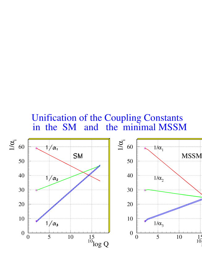
Figure 5.1: Evolution of the inverse of the three coupling constants in the Standard Model (left) and in the supersymmetric extension of the SM (MSSM) (right). Only in the latter case unification is obtained. The SUSY particles are assumed to contribute only above the effective SUSY scale $\Lambda_{SUSY}$ of about 1 TeV, which causes a change in the slope in the evolution of couplings. The thickness of the lines represents the error in the coupling constants as of 1991 [48].

5.2 Particle assignment

The minimal Supersymmetric $SU(5)$ model is the simplest framework where the unification of the Standard Model Interactions is realized. Using the quantum numbers of the SM particles Georgi and Glashow [49] showed how the matter is unified partially in two irreducible representations $\mathbf{\bar{5}}$ and $\mathbf{10}$. Using the $SU(3)\times SU(2)$ decomposition of these representations, the fermions of one family are accommodated as:

$$\mathbf{10}=(\bar{3},1)\bigoplus(3,2)\bigoplus(1,1)=(u^{C}_{i})_{L}\bigoplus(u_{i},d_{i})_{L}\bigoplus(e^{C})_{L}$$

$$\mathbf{10}=\frac{1}{\sqrt{2}}\left(\begin{array}[]{ccccc}0&u^{C}_{3}&-u^{C}_{2}&u_{1}&d_{1}\\ -u^{C}_{3}&0&u^{C}_{1}&u_{2}&d_{2}\\ u^{C}_{2}&-u^{C}_{1}&0&u_{3}&d_{3}\\ -u_{1}&-u_{2}&-u_{3}&0&e^{C}\\ -d_{1}&-d_{2}&-d_{3}&-e^{C}&0\end{array}\right)_{L}$$

$$\mathbf{\overline{5}}=(\bar{3},1)\bigoplus(1,2)=(d^{C}_{i})_{L}\bigoplus(\nu,e)_{L}$$

$$\mathbf{\overline{5}}=\left(\begin{array}[]{c}d^{C}_{1}\\ d^{C}_{2}\\ d^{C}_{3}\\ e^{-}\\ -\nu\end{array}\right)_{L}$$

$SU(5)$ is a Lie group of rank $4$, with $24$ generators. Therefore we will have $24$ gauge fields in our model, the usual Standard Model gauge bosons plus 12 additional gauge bosons:

$$A_{\mu}(24)=\frac{1}{2}\lambda^{a}A^{a}_{\mu},\ \ \ \ a=1,2\ldots 24.$$ (5.1)

where the $\lambda^{a}$ are given by:

$$\lambda_{1}=\left(\begin{array}[]{ccccc}0&1&0&0&0\\ 1&0&0&0&0\\ 0&0&0&0&0\\ 0&0&0&0&0\\ 0&0&0&0&0\end{array}\right)\qquad\lambda_{2}=\left(\begin{array}[]{ccccc}0&-i&0&0&0\\ i&0&0&0&0\\ 0&0&0&0&0\\ 0&0&0&0&0\\ 0&0&0&0&0\end{array}\right)$$

$$\lambda_{3}=\left(\begin{array}[]{ccccc}1&0&0&0&0\\ 0&-1&0&0&0\\ 0&0&0&0&0\\ 0&0&0&0&0\\ 0&0&0&0&0\end{array}\right)\qquad\lambda_{4}=\left(\begin{array}[]{ccccc}0&0&1&0&0\\ 0&0&0&0&0\\ 1&0&0&0&0\\ 0&0&0&0&0\\ 0&0&0&0&0\end{array}\right)$$

$$\lambda_{5}=\left(\begin{array}[]{ccccc}0&0&-i&0&0\\ 0&0&0&0&0\\ i&0&0&0&0\\ 0&0&0&0&0\\ 0&0&0&0&0\end{array}\right)\qquad\lambda_{6}=\left(\begin{array}[]{ccccc}0&0&0&0&0\\ 0&0&1&0&0\\ 0&1&0&0&0\\ 0&0&0&0&0\\ 0&0&0&0&0\end{array}\right)\qquad$$

$$\lambda_{7}=\left(\begin{array}[]{ccccc}0&0&0&0&0\\ 0&0&-i&0&0\\ 0&i&0&0&0\\ 0&0&0&0&0\\ 0&0&0&0&0\end{array}\right)\qquad\lambda_{8}=\frac{1}{\sqrt{3}}\left(\begin{array}[]{ccccc}1&0&0&0&0\\ 0&1&0&0&0\\ 0&0&-2&0&0\\ 0&0&0&0&0\\ 0&0&0&0&0\end{array}\right)$$

$$\lambda_{9}=\left(\begin{array}[]{ccccc}0&0&0&1&0\\ 0&0&0&0&0\\ 0&0&0&0&0\\ 1&0&0&0&0\\ 0&0&0&0&0\end{array}\right)\qquad\lambda_{10}=\left(\begin{array}[]{ccccc}0&0&0&-i&0\\ 0&0&0&0&0\\ 0&0&0&0&0\\ i&0&0&0&0\\ 0&0&0&0&0\end{array}\right)$$

$$\lambda_{11}=\left(\begin{array}[]{ccccc}0&0&0&0&1\\ 0&0&0&0&0\\ 0&0&0&0&0\\ 0&0&0&0&0\\ 1&0&0&0&0\end{array}\right)\qquad\lambda_{12}=\left(\begin{array}[]{ccccc}0&0&0&0&-i\\ 0&0&0&0&0\\ 0&0&0&0&0\\ 0&0&0&0&0\\ i&0&0&0&0\end{array}\right)$$

$$\lambda_{13}=\left(\begin{array}[]{ccccc}0&0&0&0&0\\ 0&0&0&1&0\\ 0&0&0&0&0\\ 0&1&0&0&0\\ 0&0&0&0&0\end{array}\right)\qquad\lambda_{14}=\left(\begin{array}[]{ccccc}0&0&0&0&0\\ 0&0&0&-i&0\\ 0&0&0&0&0\\ 0&i&0&0&0\\ 0&0&0&0&0\end{array}\right)$$

$$\lambda_{15}=\left(\begin{array}[]{ccccc}0&0&0&0&0\\ 0&0&0&0&1\\ 0&0&0&0&0\\ 0&0&0&0&0\\ 0&1&0&0&0\end{array}\right)\qquad\lambda_{16}=\left(\begin{array}[]{ccccc}0&0&0&0&0\\ 0&0&0&0&-i\\ 0&0&0&0&0\\ 0&0&0&0&0\\ 0&i&0&0&0\end{array}\right)$$

$$\lambda_{17}=\left(\begin{array}[]{ccccc}0&0&0&0&0\\ 0&0&0&0&0\\ 0&0&0&1&0\\ 0&0&1&0&0\\ 0&0&0&0&0\end{array}\right)\qquad\lambda_{18}=\left(\begin{array}[]{ccccc}0&0&0&0&0\\ 0&0&0&0&0\\ 0&0&0&-i&0\\ 0&0&i&0&0\\ 0&0&0&0&0\end{array}\right)$$

$$\lambda_{19}=\left(\begin{array}[]{ccccc}0&0&0&0&0\\ 0&0&0&0&0\\ 0&0&0&0&1\\ 0&0&0&0&0\\ 0&0&1&0&0\end{array}\right)\qquad\lambda_{20}=\left(\begin{array}[]{ccccc}0&0&0&0&0\\ 0&0&0&0&0\\ 0&0&0&0&-i\\ 0&0&0&0&0\\ 0&0&i&0&0\end{array}\right)$$

$$\lambda_{21}=\left(\begin{array}[]{ccccc}0&0&0&0&0\\ 0&0&0&0&0\\ 0&0&0&0&0\\ 0&0&0&0&1\\ 0&0&0&1&0\end{array}\right)\qquad\lambda_{22}=\left(\begin{array}[]{ccccc}0&0&0&0&0\\ 0&0&0&0&0\\ 0&0&0&0&0\\ 0&0&0&0&-i\\ 0&0&0&i&0\end{array}\right)$$

$$\lambda_{23}=\left(\begin{array}[]{ccccc}0&0&0&0&0\\ 0&0&0&0&0\\ 0&0&0&0&0\\ 0&0&0&1&0\\ 0&0&0&0&-1\end{array}\right)\qquad\lambda_{24}=\frac{1}{\sqrt{15}}\left(\begin{array}[]{ccccc}-2&0&0&0&0\\ 0&-2&0&0&0\\ 0&0&-2&0&0\\ 0&0&0&3&0\\ 0&0&0&0&3\end{array}\right)$$

The $SU(3)\times SU(2)$ decomposition of the 24-plet is given by:

$$24=(8,1)\bigoplus(3,2)\bigoplus(\bar{3},2)\bigoplus(1,3)\bigoplus(1,1)$$

$$A(24)=G_{ij}\bigoplus(X_{i},Y_{i})\bigoplus(\bar{Y}_{i},\bar{X}_{i})\bigoplus(W^{+},W^{3},W^{-})\bigoplus B^{0}$$

The $SU(3)$ octet $G_{ij}$ are identified with the gluons. The $SU(2)$ doublet $(X_{i},Y_{i})$ represents the two superheavy $SU(3)$ triplets $X$ and $Y$ gauge bosons with electric charges $4/3$ and $1/3$ respectively. The $SU(2)$ triplet $(W^{+},W^{3},W^{-})$ are identified with the SM $SU(2)$ vector bosons and finally $B^{0}$ is the $U(1)$ vector boson.

Now in order to know if our model reproduces the well known low-energy physics, we must break the symmetry spontaneously to the Standard Model gauge group $SU(3)_{C}\times SU(2)_{L}\times U(1)_{Y}$. In order to achieve this we define the minimal Higgs sector, which is composed of three representations, $\bf{5}_{H}$, $\bf{\bar{5}}_{H}$ and the adjoint representation $\bf{\Sigma(24)}$:

$$\bf{5}_{H}=\left(\begin{array}[]{c}T_{1}\\ T_{2}\\ T_{3}\\ H_{2}^{+}\\ H_{2}^{0}\end{array}\right)\qquad\bf{\bar{5}}_{H}=\left(\begin{array}[]{c}\overline{T}_{1}\\ \overline{T}_{2}\\ \overline{T}_{3}\\ H_{1}^{-}\\ -H_{1}^{0}\end{array}\right)$$

$$\bf{\Sigma(24)}=\left(\begin{array}[]{cc}\Sigma_{8}&\Sigma_{(3,2)}\\ \Sigma_{(\bar{3},2)}&\Sigma_{3}\\ \end{array}\right)+\frac{1}{2\sqrt{15}}\left(\begin{array}[]{cc}2&0\\ 0&-3\\ \end{array}\right)\Sigma_{24}$$

Knowing all the particles of our model we are ready to write down the interactions and analyze the possible predictions coming from new interactions.

5.3 The $SU(5)$ Lagrangian

Using the tools given in Chapter 1 and introducing a superfield for each representation of $SU(5)$, we can write the lagrangian of our model [50, 51]:

$${\cal L}_{SUSY}^{SU(5)} = \frac{1}{4}\int d^{2}\theta~{}Tr(W^{\alpha}_{5}W_{5,{\alpha}})\ +\ \frac{1}{4}\int d^{2}\bar{\theta}~{}Tr(\bar{W}^{\alpha}_{5}\bar{W}_{5,{\alpha}})$$ (5.2)

$$+ \sum_{\Psi=\bar{5},5_{H},\bar{5}_{H}}\int d^{2}\theta\ d^{2}\bar{\theta}\ \Psi^{\dagger}_{i}\ e^{g_{5}A(24)}\ \Psi_{i}$$

$$+ \sum_{\Phi=10,\Sigma}Tr\int d^{2}\theta\ d^{2}\bar{\theta}\ \Phi^{\dagger}_{i}\ e^{g_{5}A(24)}\ \Phi_{i}$$

$$+ \int d^{2}\theta\ {\cal W}_{5}+\int d^{2}\bar{\theta}\ \bar{{\cal W}}_{5}$$

The most general (in the renormalizable limit) superpotential ${\cal W}_{5}$ of $SU(5)$ which is R-parity invariant, ${\cal W}_{5}$ has two important pieces, the corresponding to the Higgs self-interactions and other describing Yukawa couplings:

$${\cal W}_{5}={\cal W}_{H}+{\cal W}_{Y}$$ (5.3)

The superpotential of the Higgs sector reads as:

$${\cal W}_{H}=\frac{m_{\Sigma}}{2}\ Tr\Sigma^{2}\ +\ \frac{\lambda}{3}\ Tr\Sigma^{3}\ +\ \eta\ \bar{5}_{H}\Sigma 5_{H}\ +\ m_{H}\bar{5}_{H}5_{H}$$ (5.4)

while the Yukawa superpotential is:

$${\cal W}_{Y}=10\Gamma_{U}105_{H}+10\Gamma_{D}\bar{5}\bar{5}_{H}$$ (5.5)

where $\Gamma^{\prime}s$ are $3\times 3$ Yukawa matrices.

In the supersymmetric standard model language the Yukawa sector can be rewritten as

$${\cal W}_{Y}= QY_{U}U^{C}H\ +\ \bar{H}QY_{D}D^{C}\ +\ \bar{H}LY_{E}E^{C}$$ (5.6)

$$+ Q\underline{A}QT\ +\ U^{C}\underline{B}E^{C}T\ +\ Q\underline{C}L\bar{T}+U^{C}\underline{D}D^{C}\bar{T}$$

where except for the heavy triplets $T$ and $\bar{T}$ the rest are the MSSM superfields in the usual notation. The generation matrices $Y_{U,D,E}$ and $\underline{A}$, $\underline{B}$, $\underline{C}$ and $\underline{D}$ can in general be arbitrary. In the minimal SU(5) defined above one finds $\underline{A}=\underline{B}=Y_{U}=Y_{U}^{T}=\Gamma_{U}$, and $\underline{C}=\underline{D}=Y_{D}=Y^{T}_{E}=\Gamma_{D}$ at the GUT scale.

From these interactions we can find the different effective operators contributing to the decay of the proton. These are LLLL and RRRR operators:

$$\frac{1}{M_{T}}\int d^{2}\theta\ (Q\ \underline{A}\ Q)\ (Q\ \underline{C}\ L)$$ (5.7)

$$\frac{1}{M_{T}}\int d^{2}\theta\ ({U^{C}}\ \underline{B}\ E^{C})\ ({U^{C}}\ \underline{D}\ D^{C})$$ (5.8)

In the next Chapter we will study all the properties of these operators, and we will analyze the predictions in the minimal model.

5.4 Symmetry Breaking

We need the following symmetry breaking:

$$SU(5)\times SUSY\Longrightarrow SU(3)_{C}\times SU(2)_{L}\times U(1)_{Y}\times SUSY$$

To study this we have to use ${\cal W}_{H}$ and calculate the relevant F-terms and set them to zero to maintain supersymmetry down to the electroweak scale. Computing the F-terms and using the condition $Tr\Sigma=0$ we find the possible solutions which give us the symmetry breaking preserving SUSY:

Case 1.

$$\langle\Sigma\rangle=0$$ (5.9)

In this case the $SU(5)$ symmetry remains unbroken.

Case 2.

$$\langle\Sigma\rangle=\frac{m_{\Sigma}}{3\lambda}\left(\begin{array}[]{ccccc}1&0&0&0&0\\ 0&1&0&0&0\\ 0&0&1&0&0\\ 0&0&0&1&0\\ 0&0&0&0&-4\end{array}\right)$$ (5.15)

In this case $SU(5)$ breaks down to $SU(4)\times U(1)$, and the last possible solution is:

Case 3.

$$\langle\Sigma\rangle=\frac{m_{\Sigma}}{\lambda}\left(\begin{array}[]{ccccc}2&0&0&0&0\\ 0&2&0&0&0\\ 0&0&2&0&0\\ 0&0&0&-3&0\\ 0&0&0&0&-3\end{array}\right)$$ (5.21)

This is the desired vacuum since $SU(5)$ is broken to $SU(3)_{C}\times SU(2)_{L}\times U(1)_{Y}$. In the supersymmetric limit all vacua are degenerate. To complete the symmetry breaking, the $G_{SM}$ must be broken to $SU(3)_{C}\times U(1)_{em}$. This is caused by the following expectation values:

$$\langle\bf{5}_{H}\rangle=\left(\begin{array}[]{c}0\\ 0\\ 0\\ 0\\ \frac{v_{2}}{\sqrt{2}}\end{array}\right)\qquad\langle\bf{\bar{5}}_{H}\rangle=\left(\begin{array}[]{c}0\\ 0\\ 0\\ 0\\ -\frac{v_{1}}{\sqrt{2}}\end{array}\right)$$ (5.32)

The fact that from ${\cal W}_{Y}$ we get $\underline{A}=\underline{B}=Y_{U}$, $\underline{C}=Y_{E}$, $\underline{D}=Y_{D}$, is simply a statement of SU(5) symmetry. On the other hand $Y_{U}=Y_{U}^{T}$ and $Y_{D}=Y^{T}_{E}$ result from the SU(4) Pati-Salam like symmetry left unbroken by $\langle 5_{H}\rangle$ and $\langle\bar{5}_{H}\rangle$. Under this symmetry $d^{c}\leftrightarrow e$, $u\leftrightarrow u^{c}$, $d\leftrightarrow e^{c}$. Of course, this symmetry is broken by $\langle\Sigma_{\alpha}^{\alpha}\rangle\neq\langle\Sigma_{4}^{4}\rangle$, where $\alpha=1,2,3$; this becomes relevant when we include higher dimensional operators suppressed by $\langle\Sigma\rangle/M_{Pl}$, which will be considered in the next section.

Knowing how $SU(5)$ is broken to the Standard Model gauge group, we can compute the masses of different Higgs superfields in our theory. From the expression of ${\cal W}_{H}$ we can compute the Triplet and the $\mu$ mass:

$$M_{T}=2\eta\frac{m_{\Sigma}}{\lambda}+m_{H}$$ (5.33)

and

$$\mu=m_{H}-3\eta\frac{m_{\Sigma}}{\lambda}$$ (5.34)

The triplet mass $M_{T}$ must be close to the GUT scale, while $\mu$ must be close to $m_{W}$. From the above relations we see that only when the parameters of the potential are fine-tuned, we can explain this difference in the masses. It is the Fine Tuning problem of GUTs. As we see here we need a lot of fine-tuning to explain how the Triplet is much heavier than the doublet, this is the so-called Doublet-Triplet Splitting or Hierarchy Problem. Supersymmetry only helps us to stabilize the splitting againts radiative corrections, but by itself does not explain its origin.

When the symmetry is broken the $X$ and $Y$ gauge bosons become massive,

$$M_{X}=M_{Y}=5\sqrt{2}g_{5}\frac{m_{\Sigma}}{\lambda}$$ (5.35)

while we find for the members of $\Sigma$

$$m_{8}=m_{3}=\frac{5}{2}m_{\Sigma}$$ (5.36)

Note that in this case the weak triplet and color octet masses are equal.

5.5 Fermion masses

As we mentioned before in the Minimal Supersymmetric $SU(5)$ model we find the relation $Y_{D}=Y^{T}_{E}=\Gamma_{D}$ at the GUT scale. When $\bar{5}_{H}$ gets the expectation value $\langle\bar{5}_{H}\rangle$= diag $\left(0,0,0,0,-\frac{v_{1}}{\sqrt{2}}\right)$ the quark and lepton masses are related as:

$$m_{e}=m_{d},\ \ \ m_{\mu}=m_{s},\ \ \ m_{\tau}=m_{b}$$ (5.37)

The first two relations are wrong. Note that the incorrect relation $\frac{m_{e}}{m_{\mu}}=\frac{m_{d}}{m_{s}}$ is predicted to be valid at any scale. On the other hand the relation for the third generation can be considered a great success of the theory.

We can imagine many ways to improve the mass relations for the first two generations [51], but the simplest and most suggestive one is to include $1/M_{Pl}$ suppressed operators which are likely to be present; after all due to the small size of the Yukawa couplings, these operators should be more important for the first two generations where the theory fails, and they require no change in the structure of the theory. Note that the value of the ratio $\frac{M_{GUT}}{M_{Pl}}\sim 10^{-3}-10^{-2}$ is even bigger than the Yukawa couplings of the first generation.

The explicit form of the renormalizable, and all the relevant non-renormalizable terms are [52]:

$${\cal W}_{Y} = \epsilon_{ijklm}\left(10_{a}^{ij}f_{ab}10_{b}^{kl}5_{H}^{m}+10_{a}^{ij}f_{1ab}10_{b}^{kl}{\Sigma^{m}_{n}\over M_{Pl}}5_{H}^{n}+10_{a}^{ij}f_{2ab}10_{b}^{kn}5_{H}^{l}{\Sigma^{m}_{n}\over M_{Pl}}\right)$$ (5.38)

$$+ \bar{5}_{Hi}10_{a}^{ij}g_{ab}\bar{5}_{bj}+\bar{5}_{Hi}{\Sigma^{i}_{j}\over M_{Pl}}10_{a}^{jk}g_{1ab}\bar{5}_{bk}+\bar{5}_{Hi}10_{a}^{ij}g_{2ab}{\Sigma_{j}^{k}\over M_{Pl}}\bar{5}_{bk}\$$

where $i,j,k,l,m,n$ are SU(5) indices, and $a,b=1,2,3$ are generation indices.

After taking the SU(5) vev $\langle\Sigma\rangle=\sigma$ diag$(2,2,2,-3,-3)$ we get at $M_{GUT}$ scale.

$$Y_{U} = 4\left(f+f^{T}\right)-12{\sigma\over M_{Pl}}\left(f_{1}+f_{1}^{T}\right)-2{\sigma\over M_{Pl}}\left(4f_{2}-f_{2}^{T}\right)\$$

$$\underline{A} = 4\left(f+f^{T}\right)+8{\sigma\over M_{Pl}}\left(f_{1}+f_{1}^{T}\right)+2{\sigma\over M_{Pl}}\left(f_{2}+f_{2}^{T}\right)\$$

$$\underline{B} = 4\left(f+f^{T}\right)+8{\sigma\over M_{Pl}}\left(f_{1}+f_{1}^{T}\right)+4{\sigma\over M_{Pl}}\left(3f_{2}-2f_{2}^{T}\right)\$$

$$Y_{D} = -g+3{\sigma\over M_{Pl}}g_{1}-2{\sigma\over M_{Pl}}g_{2}\$$

$$Y_{E} = -g+3{\sigma\over M_{Pl}}g_{1}+3{\sigma\over M_{Pl}}g_{2}\$$

$$\underline{C} = -g-2{\sigma\over M_{Pl}}g_{1}+3{\sigma\over M_{Pl}}g_{2}\$$

$$\underline{D} = -g-2{\sigma\over M_{Pl}}g_{1}-2{\sigma\over M_{Pl}}g_{2}\$$ (5.39)

using $\lambda\ \sigma=m_{\Sigma}$.

Note the relation $Y_{E}-Y_{D}=\underline{C}-\underline{D}$

In the limit $M_{Pl}\to\infty$ we recover the old relations, but for finite $\sigma/M_{Pl}\approx 10^{-3}-10^{-2}$ one can correct the relations between Yukawas and at the same time have some freedom for the couplings to the heavy triplets.

Clearly, due to SU(5) breaking through $\langle\Sigma\rangle$, the $T$, $\bar{T}$ couplings are different from the $H$, $\bar{H}$ couplings. However, under the SU(4) symmetry discussed before $\underline{A}\leftrightarrow\underline{B}$, $\underline{C}\leftrightarrow\underline{D}$ and $Y_{U}\leftrightarrow Y_{U}^{T}$. Only the terms that probe $\langle\Sigma_{\alpha}^{\alpha}\rangle-\langle\Sigma_{4}^{4}\rangle$ can spoil that; this is why $f_{1}$ and $g_{1}$ still keep $Y_{U}=Y_{U}^{T}$, $\underline{A}=\underline{B}$ and $\underline{C}=\underline{D}$.

Now we are ready to improve the mass relations for the first two families. In order to get the correct relation $\frac{m_{e}}{m_{\mu}}\simeq\frac{1}{9}\frac{m_{d}}{m_{s}}$, we must impose specific values to the coupling $g_{2}$ since:

$$Y_{D}-Y_{E}=-\frac{5}{\lambda}\frac{m_{\Sigma}}{M_{Pl}}g_{2}$$ (5.40)

If we assume that $Y_{D}$ and $Y_{E}$ are diagonals, and using the relations $m_{e}=\frac{m_{d}}{3}$ and $m_{\mu}=3m_{s}$, $g_{2}$ must satisfy the following relations:

$$(g_{2})_{11}=-\frac{2\lambda}{15}\frac{m_{d}M_{Pl}}{\langle\bar{H}\rangle\ m_{\Sigma}}$$ (5.41)

and

$$(g_{2})_{22}=\frac{2\lambda}{5}\frac{m_{s}M_{Pl}}{\langle\bar{H}\rangle\ m_{\Sigma}}$$ (5.42)

Note how the parameters of the scalar potential enter in the expressions for fermion masses.

5.6 $\sin^{2}\theta_{W}$

In the Standard Model the Weinberg angle $\theta_{W}$ is a free parameter, which plays an important role in weak interactions. From experiment we know that $\sin^{2}{\theta_{W}}_{\overline{MS}}(M_{z})=0.23117\pm 0.0016$ [53].

Let us see what happens in $SU(5)$. In the Standard model we define $\tan\theta_{W}=\frac{g_{U(1)}}{g_{SU(2)}}$, the electromagnetic charge operator $Q_{em}$ = $T_{3W}+\frac{Y}{2}$ must be part of the $SU(5)$ operators, therefore $TrQ_{em}=0$.

Now using for example the fundamental representation $\bf{5}_{H}$ we can predict $Q_{em}(T)=-\frac{1}{3}$, at the same time using ${\bf\bar{5}}$ representation we can predict $Q_{em}(d^{C})=\frac{1}{3}Q_{em}(e)$. This is one of the most beautiful predictions of GUTs, the quantization of the electric charge.

For any fundamental representation we get:

$$Q_{em}({\bf 5})=-\frac{1}{3}\left(\begin{array}[]{ccccc}1&0&0&0&0\\ 0&1&0&0&0\\ 0&0&1&0&0\\ 0&0&0&-3&0\\ 0&0&0&0&0\end{array}\right)$$

$$T_{3W}({\bf 5})=\frac{\lambda_{23}}{2}=\frac{1}{2}\left(\begin{array}[]{ccccc}0&0&0&0&0\\ 0&0&0&0&0\\ 0&0&0&0&0\\ 0&0&0&1&0\\ 0&0&0&0&-1\end{array}\right)$$

knowing these two operators, we see that the hypercharge operator must be:

$$\frac{Y}{2}({\bf 5})=\frac{1}{6}\left(\begin{array}[]{ccccc}-2&0&0&0&0\\ 0&-2&0&0&0\\ 0&0&-2&0&0\\ 0&0&0&3&0\\ 0&0&0&0&3\end{array}\right)=\sqrt{\frac{5}{3}}\frac{\lambda_{24}}{2}$$

as in $SU(5)$ all the couplings are equal, we can get the relation between $g_{U(1)}$ and $g_{SU(2)}$. From the relations listed above we can write the following expressions:

$$g_{U(1)}\frac{Y}{2}=g_{5}\frac{\lambda_{24}}{2}$$ (5.43)

$$g_{SU(2)}\frac{T_{3W}}{2}=g_{5}\frac{\lambda_{23}}{2}$$ (5.44)

concluding that $g_{U(1)}=\sqrt{\frac{3}{5}}g_{5}$ and $g_{SU(2)}=g_{5}$, so $\tan^{2}\theta_{W}=\frac{3}{5}$ or $\sin^{2}\theta_{W}=\frac{3}{8}$. It is one of the most important predictions of supersymmetric Grand Unified Theories and in particular of SUSY $SU(5)$. Note that this value is at the GUT scale, when we use the renormalization group equations and compute the value of this quantity at the electroweak scale, we see that it agrees with the experimental measurements [54, 55].

Chapter 6 Proton Decay in the Superworld

6.1 B violating operators

As we know the Baryon (B) and Lepton (L) numbers are conserved in the Standard Model. It is a consequence of the particle assignment and the gauge principle. However these symmetries could be broken at a high scale $M\gg m_{W}$. If at the high scale this happens, then we will have an effective operator ${\cal L}_{eff}$ which describes the new possible interactions:

$${\cal L}_{eff}=c_{d}\frac{{\cal O}^{d}}{M^{d-D}}$$ (6.1)

where ${\cal O}^{d}$ represents an operator of mass dimension $d$, $c_{d}$ is a coefficient, and $D$ is the space-time dimension. Note that in our “real” world we have $D=4$.
If the Baryon number is broken, we have a new prediction, the decay of the proton. This is the case of grand unified models such as $SU(5)$ and $SO(10)$, where from the matter unification we get new effective operators of the type 6.1 [56, 57]. In the case of non-conservation of Leptonic number, we have the possibility to explain the smallness of neutrino masses, due to the presence of a large Majorana mass term [58, 59, 60, 61].

Using the superfields of the Minimal Supersymmetric Standard Model $[Q=(U,D)$,  $L=(N,E)$,  $U^{C}$,  $D^{C}$,  $E^{C}]$, we can write down all the possible effective operators contributing to the decay of the proton, which are $SU(3)_{C}\times SU(2)_{L}\times U(1)_{Y}$ invariant [62, 63, 64, 65, 66, 67].

$d=4$ operators:

$$\int d^{2}\theta\ \epsilon_{\alpha\beta\gamma}\ U_{\alpha}^{C}\ D_{\beta}^{C}\ D_{\gamma}^{C}$$ (6.2)

$$\int d^{2}\theta\ \epsilon_{mn}\ Q_{m}\ D^{C}\ L_{n}$$ (6.3)

$$\int d^{2}\theta\ \epsilon_{mn}\ E^{C}\ L_{m}\ L_{n}$$ (6.4)

$d=5$ operators:

$$\frac{C^{ijkl}_{LLLL}}{M}\int d^{2}\theta\ \epsilon_{mn}\ \epsilon_{pq}\ \epsilon_{\alpha\beta\gamma}\ Q_{im\alpha}\ Q_{jn\beta}\ Q_{kp\gamma}\ L_{lq}$$ (6.5)

$$\frac{C^{ijkl}_{RRRR}}{M}\int d^{2}\theta\ \epsilon_{\alpha\beta\gamma}U_{i\alpha}^{C}\ D_{j\beta}^{C}\ U_{k\gamma}^{C}\ E^{C}_{l}$$ (6.6)

$d=6$ operators:

$$\frac{1}{M^{2}}\int d^{2}\theta\ d^{2}\bar{\theta}\ \epsilon_{\alpha\beta\gamma}\ \epsilon_{mn}\ Q_{\alpha m}^{\dagger}\ U_{\beta}^{C}\ Q_{\gamma n}^{\dagger}\ E^{C}$$ (6.7)

$$\frac{1}{M^{2}}\int d^{2}\theta\ d^{2}\bar{\theta}\ \epsilon_{\alpha\beta\gamma}\ \epsilon_{mn}\ Q_{\alpha m}^{\dagger}\ U_{\beta}^{C}\ L_{n}^{\dagger}\ D_{\gamma}^{C}$$ (6.8)

where $\alpha$, $\beta$ and $\gamma$ are color indices; m, n, p and q isospin indices, while i, j, k and l represent generation indices.

Note that the product of two $d=4$ operators and $d=6$ operators lead to proton decay at tree level. In the case of the dimension $d=4$ operators we have contributions with two fermions and one scalar field, the exchange of the scalar field can mediate proton decay. The $d=6$ operators directly yield terms with four fermions contributing to the decay of the proton. However $d=5$ operators are quite special, in each term we have two fermions and two scalars fields, therefore they contribute only at one-loop once we dress these operators.

In the case that extra spacetime dimensions are considered we see that there will be many new contributions to proton decay, without the suppression factor [68]. This is in our opinion the most important phenomenological problem of many models with extra dimensions.

Knowing all the possible operators contributing to the nucleon decay, the general expression for the proton lifetime could be written as:

$$\tau_{p}\propto|{\cal A}_{d=4}+{\cal A}_{d=5}+{\cal A}_{d=6}|^{-2}$$ (6.9)

where ${\cal A}_{i}$ are the different amplitudes. Note that in four dimensions ${\cal A}_{4}$ does not have any suppression factor, therefore the coefficients related with these contributions must be very small or maybe it is more natural find a symmetry to forbid these operators.

The second possibility is realized, if we introduce a symmetry called Matter Parity (see section 3.6):

$$M=(-1)^{3(B-L)}$$ (6.10)

where $M=-1$ for $Q$, $L$, $U^{C}$, $D^{C}$, $E^{C}$  and  $M=1$ for $H$, $\overline{H}$ and $G_{\mu}$. If we assume that this symmetry is conserved, we remove the $d=4$ contributions, retaining the $d=5$ contributions as the most important ones.

Note that relation between $R$ and $M$ parities, $R=(-1)^{2S}M$. The case where the $R$ parity is not an exact symmetry has been analyzed in reference [69]. However the most interesting case is when $R$-parity is conserved. As we mentioned before in this case we have an ideal candidate to describe the Non-Baryonic Dark Matter present in the Universe. Also the conservation of this symmetry is predicts in a large class of Grand Unified Theories as Minimal SUSY $SO(10)$ [32].

6.2 $d=6$ operators

Let us analyze in detail the $d=6$ contributions. We can use as an example the hermitian of the operator 6.7, working in 4 dimensions, choosing $m=1$, $n=2$, and using the properties of the Grassmannian variables we find the following four fermions effective operator:

$$\frac{1}{M^{2}}\ \epsilon_{\alpha\beta\gamma}\ \ (e^{C})^{\dagger}\ d_{\alpha}\ (u_{\beta}^{C})^{\dagger}\ u_{\gamma}$$ (6.11)

therefore we will have a contribution to proton decay at tree level, in this case the proton decay into $\pi^{0}$ and $e^{+}$, the usual most important channel coming from the d=6 contributions in grand unified models.

$d=6$ contribution to the decay of the proton.

Usually the $d=6$ processes are mediated by new superheavy gauge and Higgs bosons present in grand unified models. There are many aspects to be considered when we compute the proton decay amplitudes. In the first place these operators are given at the GUT scale, therefore to compute the values of the lifetime, we must compute the matrix elements for each channel, and study the evolution of these operators to the proton mass scale $1$ GeV (see [70, 71, 72] for more details).

Also there is a very important point related with the fermion masses and the prediction of proton decay. Assume that the fermion mass matrices are diagonalized as:

$$U^{T}Y_{U}U_{C}=Y_{U}^{d}\;\;\;,\;\;\;D^{T}Y_{D}D_{C}=Y_{D}^{d}\;\;\;,\;\;\;E_{C}^{T}Y^{T}_{E}E=Y_{E}^{d}\;\;\;,$$ (6.12)

when $u\to U\ u$, $u^{C}\to U_{C}\ u^{C}$ and so on.

Now if we write the $d=6$ operators (eq. 6.11) in the physical basis, we get:

$$\frac{1}{M^{2}}\ (e^{C})^{\dagger}\ (E_{C}^{\dagger}\ D)\ d\ (u^{C})^{\dagger}\ (U_{C}^{\dagger}\ U)\ u$$ (6.13)

As we see in general these operators depend of the textures for $Y_{U}$, $Y_{D}$ and $Y_{E}$, this means that the proton decay predictions will be different in each model for fermion masses [73, 74].

In the Minimal Supersymmetric $SU(5)$, where from the relation of the mass matrices $Y_{U}=Y^{T}_{U}$ and $Y_{D}=Y_{E}^{T}$ we have $U_{C}=U$ and $D=E_{C}$, the $d=6$ operators are independent of the explicit form of textures, however as we mentioned in the last chapter this is not a realistic case, due to the problem of the mass relation for the first two families.

We could say that $d=6$ proton decay provides a way to test models of fermion masses, however as we know $M_{GUT}\sim 10^{16}$ GeV which gives us $\tau_{p}(d=6)\sim 10^{35}$ years, a value which is much bigger than the present experimental bounds [75]. Therefore it is difficult to test the $d=6$ predictions at present experiments. See [76, 77] for the predictions in string-derived models.

6.3 $d=5$ operators

The $d=5$ contributions are the dominant to the proton decay. They are mediated by the superpartner of the colored Higgses (Triplets), which are present in SUSY GUT models. In this case we have only $\frac{1}{M_{T}}$ as suppression, where $M_{T}$ is the Triplet mass.
Let us understand how from these operators we get the proton decay amplitudes. We can use the following operator as a example:

$$\frac{C^{ijkl}_{LLLL}}{M_{T}}\int d^{2}\theta\ \epsilon_{mn}\ \epsilon_{pq}\ \epsilon_{\alpha\beta\gamma}\ Q_{im\alpha}\ Q_{jn\beta}\ Q_{kp\gamma}\ L_{lq}$$ (6.14)

in this case using the properties of the Grassmannian variables we see that for each contribution, there are two fermionic and two bosonic (or superpartners) fields. For example if $i=j=l=1$ and $k=2$, we find the following contribution to the decay into $K^{+}$ and $\bar{\nu}$:

$$\frac{1}{M_{T}}C^{1121}_{LLLL}\ \widetilde{u}\ \widetilde{d}\ s\ \nu$$ (6.15)

Now we must dress this operator to find the four fermions operator contributing to proton decay. This is possible using gauginos and higgsinos, since these are Majorana particles:

$d=5$ contribution to the decay of the proton.

From this graph we can appreciate that these contributions are present at one-loop level, where we have superpartners inside the loops, the loop factor and the suppression $1/M_{T}$ must be considered to compute the proton decay amplitude. As we mentioned in the last section, these operators are valid at the GUT scale, therefore we must compute the matrix elements and study the running down to 1 GeV. However in this case there are many new factors to be considered. $M_{T}$ is usually the Triplet mass, which could be smaller than the GUT scale, therefore we must compute this in order to estimate the amplitudes.

In the case of $d=6$ operators we showed how the amplitudes could depend on the textures of fermion masses. For the $d=5$ contributions we see that there is something new, the sfermion masses also appear in this case. Therefore in general the $d=5$ contributions will depend on the textures for sfermions and fermions, since in a general SUSY model these textures are different.

As we see in order to compute the proton decay amplitudes we must consider many unknown factors: the loop factor, which depends on the SUSY spectrum and mixings between fermion and sfermions, the Triplet mass and the matrix elements. Therefore we can conclude that it is very difficult to test the SUSY GUT models using proton decay, since the dominant $d=5$ contributions are quite model dependent.

6.4 Proton decay in Minimal SUSY $SU(5)$

In the last chapter we studied the structure of the Minimal Supersymmetric $SU(5)$ model. We noted that new interactions which violate the baryon and lepton numbers are present, when the matter unification is realized. From these new interactions we find the $d=5$ and $d=6$ operators contributing to the decay of the proton.

As we mentioned above the most important contributions are those with $d=5$. From the superpotential of $SU(5)$ we find the LLLL and RRRR $d=5$ operators, which read as:

$$\frac{1}{M_{T}}{\underline{A}^{ij}}{\underline{C}^{kl}}\int d^{2}\theta\ (Q_{i}\ Q_{j})\ (Q_{k}\ L_{l})$$ (6.16)

$$\frac{1}{M_{T}}{\underline{B}^{ij}}{\underline{D}^{kl}}\int d^{2}\theta({U_{i}^{C}}\ E_{j}^{C})\ ({U_{k}^{C}}\ D_{l}^{C})$$ (6.17)

Knowing these operators we can write all the $d=5$ contributions for each channel. The results are listed in Appendix B. Note that we did not assume any specific SUSY model or any texture for fermion masses. Our analysis is quite general.

If the Baryon and Lepton numbers are not conserved, there are many channels for the decay of the proton:

$$p\to(K^{+},\pi^{+},\rho^{+},K^{*+})\bar{\nu_{i}}$$

$$n\to(\pi^{0},\rho^{0},\eta,\omega,K^{0},K^{*0}){\bar{\nu}_{i}}$$

where $i=1,2,3$, and

$$p\to(K^{0},\pi^{0},\eta,K^{*0},\rho^{0},\omega)e_{j}^{+}$$

$$n\to(K^{-},\pi^{-},K^{*-},\rho^{-})e_{j}^{+}$$

where $j=1,2$, while for $K^{*}$ only $j=1$. Note that there are also new channels for neutron decay.

These operators have been studied on and off for the last 20 years with culminating conclusion that the minimal SUSY $SU(5)$ is ruled out [78].

In this paper by Murayama and Pierce, the different constraints on the Triplet mass are studied. Using the unification of the gauge couplings and the proton decay experimental lower bounds they found inconsistent limits on this mass.

To give an idea of the procedure used in reference [78], we can use the renormalization group equations for the gauge couplings at one-loop (neglecting the Yukawa couplings).

Now assuming exact unification we get at one loop level:

$$3\alpha_{2}^{-1}(m_{Z})-2\alpha_{3}^{-1}(m_{Z})-\alpha_{1}^{-1}({m_{Z}})=$$

$$\frac{1}{2\pi}\Bigl{(}\frac{12}{5}\log\frac{M_{T}}{m_{Z}}-2\log\frac{m_{SUSY}}{m_{Z}}\Bigr{)}$$ (6.18)

Therefore it is possible invert the above equation and determine the colored Higgs mass. For numerical calculation, they used the two-loop RGEs for the gauge and Yukawa couplings between the SUSY and GUT scale.

Knowing the values of the gauge couplings at the scale $m_{Z}$ [53], they found that the $SU(5)$ prediction of exact unification agrees with data only for colored Higgs masses of:

$$M_{T}\leq 3.6\times 10^{15}\mbox{GeV}$$ (6.19)

The second limit on the Triplet mass is computed using the experimental lower bound for the channel $p\to K^{+}\bar{\nu_{i}}$ of $6.7\times 10^{32}$ years [75].

Computing the proton lifetime due to the $d=5$ contributions using the methods of reference [79], they found:

$$M_{T}\geq 7.6\times 10^{16}\mbox{ GeV}$$ (6.20)

in order to satisfy the experimental bounds. It was assumed nearly degenerate scalars at the weak scale, or order 1 TeV in mass.

Comparing this equation with equation (6.19), they claim that the minimal SUSY SU(5) theory is excluded by a lot.

Now in order to consider a different scenario and see the possibilities to suppress the $d=5$ operators, they considered a second case, the so called decoupling scenario [80, 81, 82].
In this case the first and second generations of superpartners could be heavy without severe fine-tuning because they do not affect the Higgs boson self-energy at one-loop level.

Since the loop factor goes like $m_{\widetilde{G}}\ m^{-2}_{\widetilde{q}}$ (when $m_{\widetilde{G}}\ll m_{\widetilde{q}}$), where $m_{\widetilde{G}}$ is the gaugino or higgsino mass, while $m_{\widetilde{q}}$ is the slepton or squark mass. Therefore we can get a large suppression by making the sfermions of the first two generations very heavy. For example if we assume $m_{\widetilde{q}_{1,2}}\sim 10$ TeV, we get an extra suppression factor of $10^{-2}$ to the amplitude.

Now computing the lower bound for the Triplet mass in the decoupling scenario, they found that:

$$M_{T}>5.7\times 10^{16}\mbox{ GeV}.$$ (6.21)

Therefore from this analysis they concluded that the Minimal Supersymmetry $SU(5)$ is ruled out.

However in the last analysis, they did not consider the most general scenario, as we mentioned in the last section the $d=5$ contribution are quite model dependent.

Murayama and Pierce assume the following in their important analysis:

• They found the different limits on the Triplet mass in the minimal SUSY $SU(5)$ model without higher dimensional operators in ${\cal W}_{5}$, which makes wrong predictions for the fermion masses of the first two generations. This is not a realistic model, or we could say that it is already ruled out.

• They computed the proton decay amplitudes in a very specific SUSY model, where the mixings between fermions and sfermions are known, however as we mentioned before in a general SUSY model the situation may be quite different.

• Assuming exact unification of the gauge couplings, they computed the limits on the Triplet mass, however if the non-renormalizable contributions to ${\cal W}_{H}$ are considered, the bounds change.

For these reasons we think that the model is not ruled out, in our opinion before ruling out the minimal realization of the idea of unification, it is better to see how constraint the model using the experimental bounds.

In the next two sections we will point out different aspects to be considered in order to satisfy the experimental bounds on proton decay.

6.5 (S)Fermion masses versus Proton decay

In this section we will show how to satisfy all the experimental bounds on proton decay. As we mentioned before the prediction of the $d=5$ contributions will depend on the explicit form of fermion and sfermions mass matrices [83, 84, 85].

Now to start our analysis we must write all the $d=5$ operators in the physical basis, therefore we must go from the flavour to the physical basis as:

$$F_{p}\ \to\ U_{F}\ F_{f}$$ (6.22)

$$\widetilde{F}_{p}\ \to\ \widetilde{U}_{F}\ \widetilde{F}_{f}$$ (6.23)

where $F$ and $\widetilde{F}$ represent the fermion and sfermion fields respectively, while $U_{F}$ and $\widetilde{U}_{F}$ are unitary matrices.

In general there is not relation between these matrices, therefore we expect that in each $d=5$ contribution we will have a combination of different mixings between fermions and sfermions, which are unknown. Note that we only know the mixings between left-handed fermions, $V_{CKM}=U^{\dagger}D$ and $V_{l}=N^{\dagger}E$, where $N$ and $E$ are the matrices which rotate $\nu_{L}$ and $e_{L}$ respectively.

Now the main point in our analysis is, how to suppress the $d=5$ operators in order to satisfy the experimental bounds.

Assuming the decoupling scenario, where the most important contributions come from the third family of superpartners, and studying all the contributions shown in Appendix B, we see that the longevity of the proton can be achieved by, say, the following conditions at 1 GeV [86]:

$$(\tilde{U}^{\dagger}\ D)_{3a}\approx 0\;\;\;\;\;\;(\tilde{D}^{\dagger}\ D)_{3a}\approx 0\;\;\;\;\;\;(\tilde{E}_{C}^{\dagger}\ E_{C})_{3a}\approx 0\;\;\;$$

$$(\tilde{N}^{\dagger}\ E)_{3a}\approx 0\;\;\;\;\;\;(\tilde{D}_{C}^{\dagger}\ D_{C})_{3a}\approx 0\;\;\;\;\;\;(\tilde{E}^{\dagger}\ E)_{3a}\approx 0\;\;\;$$

$$(\tilde{U}_{C}^{T}\ Y_{U}^{T}\ D)_{3a}\approx 0\;\;\;$$ (6.24)

and

$$A_{0}=\epsilon_{ab}(D^{T}\ \underline{C}\ \tilde{N})_{a3}(\tilde{U}^{T}\ \underline{A}\ D)_{3b}\approx 0\;\;\;$$ (6.25)

where $a,b=1,2$. Note that $\widetilde{U}$ and $\widetilde{U}_{C}$ are the matrices which rotate $\widetilde{u}$ and $\widetilde{u}^{C}$ respectively. We use the same notation for the rest of the fermions and sfermions.

In the above equations we simply mean that all the terms must be small. How small? It is hard to quantify this precisely and, honestly speaking, it seems to us a premature task.

Our aim was to demonstrate that the theory is still consistent with data and from the above formulae it is obvious. If (when) proton decay is discovered and the decay modes measured, it may be sensible to see how small should the above terms be.

Suffice it to say, that a percent suppression of the results in the minimal SUGRA (or super KM) case should be enough. This means that on the average each vertex should be suppressed by a factor of $1/3$ or so with respect to the minimal supergravity predictions. It is very difficult to say more: in fact one could be tempted to estimate that for example the combinations on the lefthand sides of the above equations need to be at least $10^{-2}$ the same combinations in super KM. However this is generally neither necessary nor sufficient. The fact is, that we have to deal with a nonlinear system, since the total decay in a specified mode is proportional to the square of a sum of single diagrams, each of them is proportional to a combination of unknown mixings. Some of these mixings contribute to different diagrams, and some depend on others, so the task of constraining them numerically seems exaggerated in view of our complete ignorance of all these parameters. What we can say for sure is that if each of the diagrams in Appendix B is suppressed by a factor of $1/100$ with respect to the minimal supergravity predictions, proton decay is not too fast and Minimal Supersymmetric SU(5) is not ruled out.

Notice further that the so called super KM basis, in which the mixing angles of fermions and sfermions are equal, for example $\widetilde{U}_{C}=U_{C}$, does not work for the proton decay, since eqs. (6.5) and (6.25) are not satisfied. If you believe in super KM, you would conclude that the theory is ruled out. It is obvious though, from our work, that this is not true in general.

Notice even further, that all the relations (6.5)-(6.25) do not require the extreme minimality conditions: $\underline{A}=\underline{B}=Y_{U}=Y^{T}_{U}$ and $\underline{C}=\underline{D}=Y_{D}=Y^{T}_{E}$. More precisely, one can opt for the improvement of the fermion mass relations and still save the proton.

One could worry that the above constraints for the sfermion and fermion mixing matrices could be in contradiction with the experimental bounds on the flavour violating low energy processes. Fortunately, this is not true. Namely, the same conditions (6.5)-(6.25) suffice to render neutral current flavour violation in-offensive (of course, the decoupling is necessary for this to be true). We studied the processes $\mu\to e\gamma$, $b\to s\gamma$, $B-\bar{B}$, $K-\bar{K}$, etc. It is easy to see, that the combinations which appear in (6.5) are exactly the ones that appear in these flavour changing processes. So they automatically take care also of these low-energy experimental data. The only flavour changing processes that could get sizeable contributions are the ones which involve up type sfermions like for example $D-\bar{D}$ or $c\to u\gamma$. These are not constrained by (6.5), but at the same time are not very much constrained by the low-energy experiments, so they do not represent a real issue at this stage.

Constraints (6.5) are not unique. One can find other relations between sfermion and fermion mixing matrices that make the proton decay amplitude zero or small. However, typically, these solutions can be dangerous for FCNC processes, since they do not automatically cancel their contributions. So one has to analyze the FCNC processes case by case. At the present day status (or ignorance) of proton decay and FCNC experiments we believe that this is premature.

The analysis in Appendix B has been done with the assumption of no left-right sfermion mixing, and gaugino higgsino mixing in the neutralino and chargino sector. This mixing can be included in a perturbative way, one can show that, up to two mass insertions, the same constraints (6.5)-(6.25) kill all the contributions to nucleon decay. This is enough to increase the nucleon lifetime above the experimental limit, since each mixing multiplies the diagram by at least $1/10$.
Actually we could ignore the left-right mixing for sfermion proportional to the small ratio $M_{Z}/m_{\widetilde{q}}$; in fact, as long as $\tan{\beta}>10$, the LR mixing can be safely put even to zero without contradicting the experimental constraints on the Higgs mass [31].

One can also worry about naturalness [87, 88, 89, 90]. Through the large top Yukawa couplings, the formula (1.1) becomes here ($i=1,2,3$) (for large $\tan{\beta}$ there are similar contributions of (s)bottom and (s)tau)

$$m_{h}^{2}\approx m_{0}^{2}+{3y_{t}^{2}\over 16\pi^{2}}\left[(\tilde{U}^{\dagger}U)_{i3}(U^{\dagger}\tilde{U})_{3i}m^{2}_{\tilde{q}_{i}}+(\tilde{U}_{C}^{\dagger}U_{C})_{i3}(U_{C}^{\dagger}\tilde{U}_{C})_{3i}\tilde{m}^{2}_{\tilde{q}^{C}_{i}}\right]$$ (6.26)

where $m_{\tilde{q}_{i}}$ and $m_{\tilde{q}^{C}_{i}}$ are left-handed and right-handed squark masses.

Now, for $m_{\tilde{q}_{a}}\approx\tilde{m}_{\tilde{q}^{C}_{a}}\approx 10$ TeV ($a=1,2$) in the decoupling regime, large $(\tilde{U}^{\dagger}U)_{a3}$ or $(\tilde{U}_{c}^{\dagger}U_{c})_{a3}$ would imply a small amount of fine-tuning ($\approx 1\%$) in (6.26). Hereafter, we accept that. No fine-tuning whatsoever, although appealing, to us seems exaggerated; after all it would eliminate large extra dimensions as a solution to the hierarchy problem.

Strictly speaking, one could then ask why not simply push $m_{\tilde{q}_{3}}$ and $m_{\tilde{q}^{C}_{3}}$ all the way up to $10$ TeV and be safe? A sensible point, we wish to have as many as possible superpartners below TeV and thus hopefully detectable at LHC. In other words, all the gauginos and Higgsinos and the third generation of sfermions are assumed to have masses lower or equal TeV, we only take $m_{\tilde{q}_{1,2}}\approx 10$ TeV.

In this case, we need to worry only about the third generation of sfermions. We also assume light gauginos and Higgsinos, $m_{\widetilde{G}}\approx 100$ GeV.

The constraints (6.5) can clearly be satisfied exactly by the sfermion mixing matrices at $1$ GeV. It is reassuring that the sfermionic sector does not break strongly SU(2). This is consistent with the SU(2) invariance of the soft masses, which dominate the total sfermion masses.

The last constraint, eq. (6.25), can even be satisfied in the approximation $\underline{C}=Y_{D}=Y_{E}$, which is true in the minimal renormalizable model, but at $M_{GUT}$, not at 1 GeV.

The relation $\underline{C}=Y_{D}=Y_{E}$ is however not stable under running. To get an idea of how big this contribution is at the electroweak scale, one can take the approximation that the Yukawas do not run. In the leading order in small Yukawas (except for $y_{t}$) one gets

$$A_{0}\approx y_{c}y_{\tau}V_{33}^{*}V_{23}V_{32}V_{21}\left[1-\left(M_{Z}/M_{GUT}\right)^{y_{t}^{2}/16\pi^{2}}\right]x_{1}^{-1/33}x_{2}^{-3}x_{3}^{4/3}$$ (6.27)

where $V$ is the CKM matrix and $x_{i}=\alpha_{i}(M_{Z})/\alpha_{U}$. There is only one non-vanishing diagram (the rest vanishes due to (6.5)) and it is proportional to $V_{13}A_{0}$: fortunately, this seems to be small enough. On top of this, in the amplitude the combination (6.25) gets multiplied with a combination of neutralino soft masses $m_{\tilde{W}_{3}}$ and $m_{\tilde{b}}$, which can be fine-tuned to an arbitrary small (or even zero) value. And, of course, we must keep in mind that $M_{T}$ can be large and $\underline{A}$ and/or $\underline{C}$ completely different than $Y_{U}$ ($Y_{E}$).

In other words, at this point the proton decay limits provide information on the properties of sfermions and not on the structure of the unified theory.

6.6 The Higgs Triplet Mass

The determination of the GUT scale and the masses ($M_{T}$) of the heavy triplets $T$ and $\bar{T}$ responsible for $d=5$ proton decay is one of the most important tasks in order to estimate the proton decay amplitude.

Specifically, if we allow an arbitrary trilinear couplings of the heavy fields in $\Sigma$ and use higher dimensional terms as a possible source of their masses [91, 92], it will turn out that $M_{T}$ may go up naturally by a factor of thirty, which would increase the proton lifetime by a factor of $10^{3}$.

Now to start our calculation, consider the non-renormalizable terms in the superpotential for the heavy sector (up to terms $1/M_{Pl}$):

$${\cal W}_{H}=\frac{m_{\Sigma}}{2}\ Tr\Sigma^{2}+\frac{\lambda}{3}Tr\Sigma^{3}+a{(Tr\Sigma^{2})^{2}\over M_{Pl}}+b{Tr\Sigma^{4}\over M_{Pl}}$$ (6.28)

Of course, if $\lambda\approx{\cal O}(1)$, we ignore higher-dimensional terms. However, in supersymmetry $\lambda$ is a Yukawa-type coupling, i.e. self-renormalizable. For small $\lambda$ ($\lambda\ll M_{GUT}/M_{Pl}$), the opposite becomes true and $a$ and $b$ terms dominate. In this case, it is a simple exercise to show that

$$m_{3}=4m_{8}$$ (6.29)

where $m_{3}$ and $m_{8}$ are the masses of the weak triplet and color octet in $\Sigma$. In the renormalizable case $m_{3}=m_{8}$.

At the one loop level, the RGE’s for the gauge couplings are

$$\alpha_{1}^{-1}(M_{Z}) = \alpha_{U}^{-1}+{1\over 2\pi}\left(-{5\over 2}\ln{\Lambda_{SUSY}\over M_{Z}}+{33\over 5}\ln{M_{GUT}\over M_{Z}}+{2\over 5}\ln{M_{GUT}\over M_{T}}\right)$$

$$\alpha_{2}^{-1}(M_{Z}) = \alpha_{U}^{-1}+{1\over 2\pi}\left(-{25\over 6}\ln{\Lambda_{SUSY}\over M_{Z}}+\ln{M_{GUT}\over M_{Z}}+2\ln{M_{GUT}\over m_{3}}\right)$$

$$\alpha_{3}^{-1}(M_{Z}) = \alpha_{U}^{-1}+{1\over 2\pi}\left(-4\ln{\Lambda_{SUSY}\over M_{Z}}-3\ln{m_{8}\over M_{Z}}+\ln{M_{GUT}\over M_{T}}\right)$$ (6.30)

Here we take for simplicity $M_{GUT}=M_{X,Y}=$ superheavy gauge bosons masses, while at the one-loop level we could as well take $\Lambda_{SUSY}=M_{Z}$. From (6.30) we obtain

$$2\pi\left(3\alpha_{2}^{-1}-2\alpha_{3}^{-1}-\alpha_{1}^{-1}\right) = -2\ln{\Lambda_{SUSY}\over M_{Z}}+{12\over 5}\ln{M_{T}\over M_{Z}}+6\ln{m_{8}\over m_{3}}$$

$$2\pi\left(5\alpha_{1}^{-1}-3\alpha_{2}^{-1}-2\alpha_{3}^{-1}\right) = 8\ln{\Lambda_{SUSY}\over M_{Z}}+36\ln{(\sqrt{m_{3}m_{8}}M_{GUT}^{2})^{1/3}\over M_{Z}}$$

This gives

$$M_{T} = M_{T}^{0}\left({m_{3}\over m_{8}}\right)^{5/2}$$ (6.32)

$$M_{GUT} = M_{GUT}^{0}\left({M_{GUT}^{0}\over 2m_{8}}\right)^{1/2}$$ (6.33)

Since, in the case (6.29) is valid, $m_{8}\approx M_{GUT}^{2}/M_{Pl}$, we can also write

$$M_{GUT}\approx\left[\left(M_{GUT}^{0}\right)^{3}M_{Pl}\right]^{1/4}$$ (6.34)

In the above equations the superscript ⁰ denotes the values in the case $m_{3}=m_{8}$. From (6.29) we get

$$M_{T}=32M_{T}^{0}\;\;\;\;\;\;M_{GUT}\approx 10M_{GUT}^{0}\;\;\;$$ (6.35)

Now, $M_{GUT}^{0}\approx 10^{16}$ GeV and it was shown last year [78] that $M_{T}>7\times 10^{16}$ GeV is sufficiently large to be in accord with the newest data on proton decay. On the other hand, since we had

$$M_{T}^{0}<3.6\times 10^{15}{\rm GeV}\;$$ (6.36)

from (6.35) we see that $m_{3}=4m_{8}$ is enough to save the theory, even in the minimal SUGRA model. Obviously, an improvement of the measurement of $\tau_{p}$ is badly needed. It is noteworthy that in this case the usual $d=6$ proton decay becomes out of reach: $\tau_{p}(d=6)>10^{38}$ yrs.

As we see there are many reasons to believe that the Minimal Supersymmetric $SU(5)$ model is not ruled out. The proton decay lifetime depends of many unknown parameters, therefore at the same time using the proton decay constraint we could learn about a sector which is orthogonal to grand unification. In other words, the improved measurements of proton decay will provide information about the nature of supersymmetry breaking (i.e., the soft masses) and the fermionic mass textures.

After our analysis different groups have been studied the same crucial issue in the minimal supersymmetric $SU(5)$ model. Our predictions about how suppress the $d=5$ contributions has been confirmed in reference [93]. In this case they computed the proton lifetime in realistic scenarios, where the needed non-renormalizable operators in the Yukawa and Higgs sector of the theory are considered. They showed several numerical examples where the experimental bounds are satisfied.

Therefore from our analysis it is clear that the minimal realization of the ideas of supersymmetric unification is not ruled out by the Proton decay experiments.

Chapter 7 Conclusions

In this thesis we studied two important phenomenological issues in the context of supersymmetric gauge theories. Invisible Higgs boson decays into neutralinos and proton decay.

We started with the study of the invisible Higgs decays into two neutralinos in the context of the minimal supersymmetric version of the Standard Model, considering new one-loop corrections to the neutral Higgs boson couplings to neutralinos in the gaugino limit. We computed these important quantum corrections and included our results in the Fortran code HDECAY [39] to compute the branching ratios for the neutral Higgs bosons. We focused on the phenomenologically most interesting case of a bino–like lightest neutralino $\tilde{\chi}_{1}^{0}$ as lightest supersymmetric particle, but our analytical results are valid for a more general gaugino–like neutralino, irrespective of whether it is the lightest supersymmetric particle. We found that these corrections can completely dominate the tree–level contribution to the coupling of the lightest CP–even Higgs boson. The corrections to the couplings of heavy CP–even Higgs boson are somewhat less significant, but can still amount to about a factor of 2. Since the CP–odd Higgs boson cannot couple to two identical sfermions the corrections are suppressed in this case. In all cases the corrections can be significant only if some sfermion masses are considerably smaller than the supersymmetric higgsino mass $|\mu|$. The Higgs couplings receive their potentially largest corrections from loops involving third generation quarks and their superpartners. In the latter case the corrections are also quite sensitive to the size of the trilinear soft breaking parameter $A_{t}$ (and $A_{b}$, if $\tan\beta\gg 1$).

The possible impact of the corrections on the invisible width of the lightest CP-even Higgs boson is dramatic, it could be enhanced to a level that should be easily measurable at future high-energy $e^{+}e^{-}$ colliders, even if the neutralino is an almost perfect bino. This would open a new window for testing the Minimal Supersymmetric Standard Model at the quantum level

Turning to applications of these calculations, our results motivated us to investigate the effect of these quantum corrections in the elastic neutralino-nucleon cross section. In this case we found [28] that these corrections might change the predicted detection rate of Dark Matter LSPs by up to a factor of two even for scenarios where the rate is close to the sensitivity of the next round of direct Dark Matter detection experiments.

A new analysis has been performed after our results were published, where also the effect of the subleading loop corrections has been analyzed. In reference [45] a different group studied the one-loop corrections to neutral Higgs bosons decays into neutralinos in the general case, where we have the decays $H^{0}_{i}\to\tilde{\chi}_{m}^{0}\tilde{\chi}_{n}^{0}$ (i=1,2,3). They confirmed our results computing the branching ratios for similar values of the parameters.

In the second part of our work we focused on proton decay in the Minimal Supersymmetric $SU(5)$ model. We studied the $d=5$ operators contributing to the decay of the proton, writing all the possible contributions for each decay channel (see Appendix B) in a general SUSY scenario. We pointed out the major sources of uncertainties in estimating the proton decay lifetime, as the ignorance of the masses of the color octet and weak triplet supermultiplets in the adjoint Higgs, and the unknown mixings between fermions and sfermions. Non-renormalizable operators are considered in order to correct the relation between the fermion masses.

We found that the Higgs triplet mass may goes up naturally by a factor of thirty, when we allow for arbitrary trilinear coupling in the presence of non-renormalizable operators, therefore in this case it is possible to satisfy the proton decay bounds, when the mixings between fermions and sfermions are known. This is the case of the minimal SUGRA model. Alternatively, if the standard value of $M_{T}$ is adopted, the conditions for the sfermion and fermion mass matrices in order to achieve the proton longevity were found. Knowing all the aspects mentioned before we can conclude that the minimal version of the ideas of Supersymmetric Grand Unification is not ruled out as claimed before. We could say that if proton decay is found, it could provide indirect information about the nature of supersymmetry breaking (i.e., the soft masses) and the fermionic mass textures. Thus opening a new way to test models for fermion and sfermion masses. We could say that our analysis is also valid for any Supersymmetric version of Grand Unified Theories as minimal SUSY $SO(10)$ [33].

Our results motivate the analysis in reference[93], where our predictions about how to suppress the $d=5$ contributions has been confirmed in several numerical examples.

We hope that these results motivate the realization of new studies in the context of supersymmetric gauge theories. The loop corrections computed by us could be important for future studies in collider physics. While our ideas of how to suppress or constrain the $d=5$ operators contributing for proton decay might be useful for understanding how it is possible test the ideas of supersymmetric unification.

Acknowledgments.

In the first place I would like to thank my family and in special my mother for the inconditional support of any kind during these years that I was far from home.

I thank my supervisor the Professor Manuel Drees for introduced me in the field of SUSY phenomenology. He was always ready to discuss my questions. I would like to thank him for the support during the development of this thesis.
I would like to thank my supervisor Professor Goran Senjanović, for his support during my Ph.D and for provide me the opportunity to work in the field of supersymmetric grand unified theories. I thank him for his friendship, all the discussions and support in the realization of this thesis. At any time he was ready to discuss my questions and ideas. I would like to thank him for the invitations to work at the ICTP.
I would like to thank the Max Planck Institut für Physics (Werner-Heisenberg-Institut) for support. I will remember forever all the moments at the institute.
I would like to thank the Abdus Salam International Centre for Theoretical Physics (ICTP) in Trieste for the support. It is a special place for me, which I will remember forever.
I thank the Prof. A. Djouadi and M. Muehlleitner for collaboration in the field of Higgs Physics.
I woud like to thank Prof. Borut Bajc for collaboration, support and for careful reading of this thesis.
I thank Pushan Majumdar for careful reading of the thesis.
I would like to thank my friends Alex, Shirley, Alina, Ariel (el Che), Alexei, Silvia, Gabriela and Andrea for their special and strong support during these years. I will remember their helps and all the special moments that we spent together.
Last but not least I would like to express my warmest thanks to Natalia.

Appendix A Passarino-Veltman Loop Formulae

The explicit form of the Passarino-Veltman loop integrals are:

$$C_{0}(p_{1},p_{2},M_{1},M_{2},M_{3})=(2\pi\mu)^{4-n}\int\frac{d^{n}l}{i\pi^{2}}\frac{1}{D_{1}D_{2}D_{3}}$$

with

$$D_{1}=l^{2}-M^{2}_{1}+i\epsilon$$

$$D_{2}=(l+p_{1})^{2}-M^{2}_{2}+i\epsilon$$

$$D_{3}=(l+p_{1}+p_{2})^{2}-M^{2}_{3}+i\epsilon$$

$$\overline{C}_{\mu}(p_{1},p_{2},M_{1},M_{2},M_{3})=(2\pi\mu)^{4-n}\int\frac{d^{n}l}{i\pi^{2}}\frac{l_{\mu}}{D_{4}D_{5}D_{6}}$$

where:

$$D_{4}=(l-p_{1})^{2}-M^{2}_{1}+i\epsilon$$

$$D_{5}=(l-p_{2})^{2}-M^{2}_{3}+i\epsilon$$

$$D_{6}=l^{2}-M^{2}_{1}+i\epsilon$$

where $p_{i}$ and $M_{i}$ are the external momenta and the masses respectively. For more details see reference [94].

Appendix B Proton Decay Diagrams

In this Appendix we present the complete set of diagrams responsible for d=5 nucleon decay in the minimal supersymmetric SU(5) theory. In our notation $T$ and $\bar{T}$ stand for heavy Higgs triplets; $\tilde{T}$ and $\tilde{\bar{T}}$ denote their fermionic partners; $\tilde{w}^{\pm}$ stands for winos, $\tilde{h}_{+,0}$ and $\tilde{\bar{h}}_{-,0}$ are light Higgsinos and $\tilde{V}_{0}$ stand for neutral gauginos.

Decay modes:

$p\to(K^{+},\pi^{+},\rho^{+},K^{*+})\bar{\nu}_{i}$  and  $n\to(\pi^{0},\rho^{0},\eta,\omega,K^{0},K^{*0})\bar{\nu}_{i}$

where $i=1,2,3$.

$$\begin{picture}(80.0,40.0)(40.0,20.0) \put(0.0,0.0){} \put(0.0,0.0){} \put(0.0,0.0){} \put(0.0,0.0){} \put(0.0,0.0){} \put(0.0,0.0){} \put(0.0,0.0){} \put(0.0,0.0){} \put(0.0,0.0){} \put(0.0,0.0){} \put(0.0,0.0){} \put(0.0,0.0){} \put(0.0,0.0){} \put(0.0,0.0){} \raise 30.0pt\hbox to0.0pt{\kern 10.0pt\makebox(0.0,0.0)[]{$\tilde{T}$}\hss} \ignorespaces \raise 10.0pt\hbox to0.0pt{\kern 10.0pt\makebox(0.0,0.0)[]{$\tilde{\bar{T}}$}\hss} \ignorespaces \raise 30.0pt\hbox to0.0pt{\kern 40.0pt\makebox(0.0,0.0)[]{$\tilde{t}$}\hss} \ignorespaces \raise 10.0pt\hbox to0.0pt{\kern 40.0pt\makebox(0.0,0.0)[]{$\tilde{\tau}$}\hss} \ignorespaces \raise 30.0pt\hbox to0.0pt{\kern 75.0pt\makebox(0.0,0.0)[]{$\tilde{w}^{+}$}\hss} \ignorespaces \raise 10.0pt\hbox to0.0pt{\kern 75.0pt\makebox(0.0,0.0)[]{$\tilde{w}^{-}$}\hss} \ignorespaces \raise 40.0pt\hbox to0.0pt{\kern-10.0pt\makebox(0.0,0.0)[]{$d_{1,2}$}\hss} \ignorespaces \raise 0.0pt\hbox to0.0pt{\kern-10.0pt\makebox(0.0,0.0)[]{$u$}\hss} \ignorespaces \raise 0.0pt\hbox to0.0pt{\kern 90.0pt\makebox(0.0,0.0)[]{$\nu_{i}$}\hss} \ignorespaces \raise 40.0pt\hbox to0.0pt{\kern 90.0pt\makebox(0.0,0.0)[]{$d_{2,1}$}\hss} \ignorespaces \end{picture}\propto(D^{T}\underline{A}\tilde{U})_{13,23}(\tilde{U}^{\dagger}D)_{32,31}(N^{T}\tilde{E}^{*})_{i3}(\tilde{E}^{T}\underline{C}^{T}U)_{31}$$

$$\begin{picture}(80.0,40.0)(40.0,20.0) \put(0.0,0.0){} \put(0.0,0.0){} \put(0.0,0.0){} \put(0.0,0.0){} \put(0.0,0.0){} \put(0.0,0.0){} \put(0.0,0.0){} \put(0.0,0.0){} \put(0.0,0.0){} \put(0.0,0.0){} \put(0.0,0.0){} \raise 30.0pt\hbox to0.0pt{\kern 25.0pt\makebox(0.0,0.0)[]{$T$}\hss} \ignorespaces \raise 35.0pt\hbox to0.0pt{\kern 45.0pt\makebox(0.0,0.0)[]{$\tilde{t}$}\hss} \ignorespaces \raise 5.0pt\hbox to0.0pt{\kern 45.0pt\makebox(0.0,0.0)[]{$\tilde{\tau}$}\hss} \ignorespaces \raise 30.0pt\hbox to0.0pt{\kern 75.0pt\makebox(0.0,0.0)[]{$\tilde{w}^{+}$}\hss} \ignorespaces \raise 10.0pt\hbox to0.0pt{\kern 75.0pt\makebox(0.0,0.0)[]{$\tilde{w}^{-}$}\hss} \ignorespaces \raise 40.0pt\hbox to0.0pt{\kern-10.0pt\makebox(0.0,0.0)[]{$d_{1,2}$}\hss} \ignorespaces \raise 0.0pt\hbox to0.0pt{\kern-10.0pt\makebox(0.0,0.0)[]{$u$}\hss} \ignorespaces \raise 0.0pt\hbox to0.0pt{\kern 90.0pt\makebox(0.0,0.0)[]{$\nu_{i}$}\hss} \ignorespaces \raise 40.0pt\hbox to0.0pt{\kern 90.0pt\makebox(0.0,0.0)[]{$d_{2,1}$}\hss} \ignorespaces \end{picture}\propto(D^{T}\underline{A}U)_{11,21}(N^{T}\tilde{E}^{*})_{i3}(\tilde{E}^{T}\underline{C}^{T}\tilde{U})_{33}(\tilde{U}^{\dagger}D)_{32,31}$$

$$\begin{picture}(80.0,40.0)(40.0,20.0) \put(0.0,0.0){} \put(0.0,0.0){} \put(0.0,0.0){} \put(0.0,0.0){} \put(0.0,0.0){} \put(0.0,0.0){} \put(0.0,0.0){} \put(0.0,0.0){} \put(0.0,0.0){} \put(0.0,0.0){} \put(0.0,0.0){} \put(0.0,0.0){} \put(0.0,0.0){} \put(0.0,0.0){} \raise 30.0pt\hbox to0.0pt{\kern 10.0pt\makebox(0.0,0.0)[]{$\tilde{T}$}\hss} \ignorespaces \raise 10.0pt\hbox to0.0pt{\kern 10.0pt\makebox(0.0,0.0)[]{$\tilde{\bar{T}}$}\hss} \ignorespaces \raise 30.0pt\hbox to0.0pt{\kern 40.0pt\makebox(0.0,0.0)[]{$\tilde{t}$}\hss} \ignorespaces \raise 10.0pt\hbox to0.0pt{\kern 40.0pt\makebox(0.0,0.0)[]{$\tilde{b}$}\hss} \ignorespaces \raise 30.0pt\hbox to0.0pt{\kern 75.0pt\makebox(0.0,0.0)[]{$\tilde{w}^{+}$}\hss} \ignorespaces \raise 10.0pt\hbox to0.0pt{\kern 75.0pt\makebox(0.0,0.0)[]{$\tilde{w}^{-}$}\hss} \ignorespaces \raise 40.0pt\hbox to0.0pt{\kern-10.0pt\makebox(0.0,0.0)[]{$d_{1,2}$}\hss} \ignorespaces \raise 0.0pt\hbox to0.0pt{\kern-10.0pt\makebox(0.0,0.0)[]{$\nu_{i}$}\hss} \ignorespaces \raise 0.0pt\hbox to0.0pt{\kern 90.0pt\makebox(0.0,0.0)[]{$u$}\hss} \ignorespaces \raise 40.0pt\hbox to0.0pt{\kern 90.0pt\makebox(0.0,0.0)[]{$d_{2,1}$}\hss} \ignorespaces \end{picture}\propto(D^{T}\underline{A}\tilde{U})_{13,23}(\tilde{U}^{\dagger}D)_{32,31}(U^{T}\tilde{D}^{*})_{13}(\tilde{D}^{T}\underline{C}N)_{3i}$$

$$\begin{picture}(80.0,40.0)(40.0,20.0) \put(0.0,0.0){} \put(0.0,0.0){} \put(0.0,0.0){} \put(0.0,0.0){} \put(0.0,0.0){} \put(0.0,0.0){} \put(0.0,0.0){} \put(0.0,0.0){} \put(0.0,0.0){} \put(0.0,0.0){} \put(0.0,0.0){} \raise 30.0pt\hbox to0.0pt{\kern 25.0pt\makebox(0.0,0.0)[]{$\bar{T}$}\hss} \ignorespaces \raise 35.0pt\hbox to0.0pt{\kern 45.0pt\makebox(0.0,0.0)[]{$\tilde{t}$}\hss} \ignorespaces \raise 5.0pt\hbox to0.0pt{\kern 45.0pt\makebox(0.0,0.0)[]{$\tilde{b}$}\hss} \ignorespaces \raise 30.0pt\hbox to0.0pt{\kern 75.0pt\makebox(0.0,0.0)[]{$\tilde{w}^{+}$}\hss} \ignorespaces \raise 10.0pt\hbox to0.0pt{\kern 75.0pt\makebox(0.0,0.0)[]{$\tilde{w}^{-}$}\hss} \ignorespaces \raise 40.0pt\hbox to0.0pt{\kern-10.0pt\makebox(0.0,0.0)[]{$d_{1,2}$}\hss} \ignorespaces \raise 0.0pt\hbox to0.0pt{\kern-10.0pt\makebox(0.0,0.0)[]{$\nu_{i}$}\hss} \ignorespaces \raise 0.0pt\hbox to0.0pt{\kern 90.0pt\makebox(0.0,0.0)[]{$u$}\hss} \ignorespaces \raise 40.0pt\hbox to0.0pt{\kern 90.0pt\makebox(0.0,0.0)[]{$d_{2,1}$}\hss} \ignorespaces \end{picture}\propto(D^{T}\underline{C}N)_{1i,2i}(U^{T}\tilde{D}^{*})_{13}(\tilde{D}^{T}\underline{A}\tilde{U})_{33}(\tilde{U}^{\dagger}D)_{32,31}$$

$$\begin{picture}(80.0,40.0)(40.0,20.0) \put(0.0,0.0){} \put(0.0,0.0){} \put(0.0,0.0){} \put(0.0,0.0){} \put(0.0,0.0){} \put(0.0,0.0){} \put(0.0,0.0){} \put(0.0,0.0){} \put(0.0,0.0){} \put(0.0,0.0){} \put(0.0,0.0){} \put(0.0,0.0){} \put(0.0,0.0){} \put(0.0,0.0){} \raise 30.0pt\hbox to0.0pt{\kern 10.0pt\makebox(0.0,0.0)[]{$\tilde{T}$}\hss} \ignorespaces \raise 10.0pt\hbox to0.0pt{\kern 10.0pt\makebox(0.0,0.0)[]{$\tilde{\bar{T}}$}\hss} \ignorespaces \raise 30.0pt\hbox to0.0pt{\kern 40.0pt\makebox(0.0,0.0)[]{$\tilde{t}$}\hss} \ignorespaces \raise 10.0pt\hbox to0.0pt{\kern 40.0pt\makebox(0.0,0.0)[]{$\tilde{b}$}\hss} \ignorespaces \raise 30.0pt\hbox to0.0pt{\kern 75.0pt\makebox(0.0,0.0)[]{$\tilde{\bar{h}}_{-}^{\dagger}$}\hss} \ignorespaces \raise 10.0pt\hbox to0.0pt{\kern 75.0pt\makebox(0.0,0.0)[]{$\tilde{h}_{+}^{\dagger}$}\hss} \ignorespaces \raise 40.0pt\hbox to0.0pt{\kern-10.0pt\makebox(0.0,0.0)[]{$d_{1,2}$}\hss} \ignorespaces \raise 0.0pt\hbox to0.0pt{\kern-10.0pt\makebox(0.0,0.0)[]{$\nu_{i}$}\hss} \ignorespaces \raise 0.0pt\hbox to0.0pt{\kern 90.0pt\makebox(0.0,0.0)[]{${\bar{u}}^{c}$}\hss} \ignorespaces \raise 40.0pt\hbox to0.0pt{\kern 90.0pt\makebox(0.0,0.0)[]{${\bar{d}}_{2,1}^{c}$}\hss} \ignorespaces \end{picture}\propto(D^{T}\underline{A}\tilde{U})_{13,23}(\tilde{U}^{\dagger}Y_{D}^{*}D_{c}^{*})_{32,31}(U_{c}^{\dagger}Y_{U}^{\dagger}\tilde{D}^{*})_{13}(\tilde{D}^{T}\underline{C}N)_{3i}$$

$$\begin{picture}(80.0,40.0)(40.0,20.0) \put(0.0,0.0){} \put(0.0,0.0){} \put(0.0,0.0){} \put(0.0,0.0){} \put(0.0,0.0){} \put(0.0,0.0){} \put(0.0,0.0){} \put(0.0,0.0){} \put(0.0,0.0){} \put(0.0,0.0){} \put(0.0,0.0){} \raise 30.0pt\hbox to0.0pt{\kern 25.0pt\makebox(0.0,0.0)[]{$\bar{T}$}\hss} \ignorespaces \raise 35.0pt\hbox to0.0pt{\kern 45.0pt\makebox(0.0,0.0)[]{$\tilde{t}$}\hss} \ignorespaces \raise 5.0pt\hbox to0.0pt{\kern 45.0pt\makebox(0.0,0.0)[]{$\tilde{b}$}\hss} \ignorespaces \raise 30.0pt\hbox to0.0pt{\kern 75.0pt\makebox(0.0,0.0)[]{$\tilde{\bar{h}}_{-}^{\dagger}$}\hss} \ignorespaces \raise 10.0pt\hbox to0.0pt{\kern 75.0pt\makebox(0.0,0.0)[]{$\tilde{h}_{+}^{\dagger}$}\hss} \ignorespaces \raise 40.0pt\hbox to0.0pt{\kern-10.0pt\makebox(0.0,0.0)[]{$d_{1,2}$}\hss} \ignorespaces \raise 0.0pt\hbox to0.0pt{\kern-10.0pt\makebox(0.0,0.0)[]{$\nu_{i}$}\hss} \ignorespaces \raise 0.0pt\hbox to0.0pt{\kern 90.0pt\makebox(0.0,0.0)[]{${\bar{u}}^{c}$}\hss} \ignorespaces \raise 40.0pt\hbox to0.0pt{\kern 90.0pt\makebox(0.0,0.0)[]{${\bar{d}}_{2,1}^{c}$}\hss} \ignorespaces \end{picture}\propto(D^{T}\underline{C}N)_{1i,2i}(U_{c}^{\dagger}Y_{U}^{\dagger}\tilde{D}^{*})_{13}(\tilde{D}^{T}\underline{A}\tilde{U})_{33}(\tilde{U}^{\dagger}Y_{D}^{*}D_{c}^{*})_{32,31}$$

$$\begin{picture}(80.0,40.0)(40.0,20.0) \put(0.0,0.0){} \put(0.0,0.0){} \put(0.0,0.0){} \put(0.0,0.0){} \put(0.0,0.0){} \put(0.0,0.0){} \put(0.0,0.0){} \put(0.0,0.0){} \put(0.0,0.0){} \put(0.0,0.0){} \put(0.0,0.0){} \put(0.0,0.0){} \put(0.0,0.0){} \put(0.0,0.0){} \raise 30.0pt\hbox to0.0pt{\kern 10.0pt\makebox(0.0,0.0)[]{$\tilde{T}^{\dagger}$}\hss} \ignorespaces \raise 10.0pt\hbox to0.0pt{\kern 10.0pt\makebox(0.0,0.0)[]{$\tilde{\bar{T}}^{\dagger}$}\hss} \ignorespaces \raise 30.0pt\hbox to0.0pt{\kern 40.0pt\makebox(0.0,0.0)[]{$\tilde{\tau}^{c}$}\hss} \ignorespaces \raise 10.0pt\hbox to0.0pt{\kern 40.0pt\makebox(0.0,0.0)[]{$\tilde{t}^{c}$}\hss} \ignorespaces \raise 30.0pt\hbox to0.0pt{\kern 75.0pt\makebox(0.0,0.0)[]{$\tilde{\bar{h}}_{-}$}\hss} \ignorespaces \raise 10.0pt\hbox to0.0pt{\kern 75.0pt\makebox(0.0,0.0)[]{$\tilde{h}_{+}$}\hss} \ignorespaces \raise 40.0pt\hbox to0.0pt{\kern-10.0pt\makebox(0.0,0.0)[]{${\bar{u}}^{c}$}\hss} \ignorespaces \raise 0.0pt\hbox to0.0pt{\kern-10.0pt\makebox(0.0,0.0)[]{${\bar{d}}_{2,1}^{c}$}\hss} \ignorespaces \raise 0.0pt\hbox to0.0pt{\kern 90.0pt\makebox(0.0,0.0)[]{$d_{1,2}$}\hss} \ignorespaces \raise 40.0pt\hbox to0.0pt{\kern 90.0pt\makebox(0.0,0.0)[]{$\nu_{i}$}\hss} \ignorespaces \end{picture}\propto(U_{c}^{\dagger}\underline{B}^{*}\tilde{E}_{c}^{*})_{13}(\tilde{E}_{c}^{T}Y_{E}N)_{3i}(D^{T}Y_{U}\tilde{U}_{c})_{13,23}(\tilde{U}_{c}^{\dagger}\underline{D}^{*}D_{c}^{*})_{32,31}$$

$$\begin{picture}(80.0,40.0)(40.0,20.0) \put(0.0,0.0){} \put(0.0,0.0){} \put(0.0,0.0){} \put(0.0,0.0){} \put(0.0,0.0){} \put(0.0,0.0){} \put(0.0,0.0){} \put(0.0,0.0){} \put(0.0,0.0){} \put(0.0,0.0){} \put(0.0,0.0){} \raise 30.0pt\hbox to0.0pt{\kern 25.0pt\makebox(0.0,0.0)[]{$\bar{T}$}\hss} \ignorespaces \raise 35.0pt\hbox to0.0pt{\kern 45.0pt\makebox(0.0,0.0)[]{$\tilde{\tau}^{c}$}\hss} \ignorespaces \raise 5.0pt\hbox to0.0pt{\kern 45.0pt\makebox(0.0,0.0)[]{$\tilde{t}^{c}$}\hss} \ignorespaces \raise 30.0pt\hbox to0.0pt{\kern 75.0pt\makebox(0.0,0.0)[]{$\tilde{\bar{h}}_{-}$}\hss} \ignorespaces \raise 10.0pt\hbox to0.0pt{\kern 75.0pt\makebox(0.0,0.0)[]{$\tilde{h}_{+}$}\hss} \ignorespaces \raise 40.0pt\hbox to0.0pt{\kern-10.0pt\makebox(0.0,0.0)[]{${\bar{u}}^{c}$}\hss} \ignorespaces \raise 0.0pt\hbox to0.0pt{\kern-10.0pt\makebox(0.0,0.0)[]{${\bar{d}}_{1,2}^{c}$}\hss} \ignorespaces \raise 0.0pt\hbox to0.0pt{\kern 90.0pt\makebox(0.0,0.0)[]{$d_{2,1}$}\hss} \ignorespaces \raise 40.0pt\hbox to0.0pt{\kern 90.0pt\makebox(0.0,0.0)[]{$\nu_{i}$}\hss} \ignorespaces \end{picture}\propto(U_{c}^{\dagger}\underline{D}^{*}D_{c}^{*})_{11,12}(D^{T}Y_{U}\tilde{U}_{c})_{23,13}(\tilde{U}_{c}^{\dagger}\underline{B}^{*}\tilde{E}_{c}^{*})_{33}(\tilde{E}_{c}^{T}Y_{E}N)_{3i}$$

$$\begin{picture}(80.0,40.0)(40.0,20.0) \put(0.0,0.0){} \put(0.0,0.0){} \put(0.0,0.0){} \put(0.0,0.0){} \put(0.0,0.0){} \put(0.0,0.0){} \put(0.0,0.0){} \put(0.0,0.0){} \put(0.0,0.0){} \put(0.0,0.0){} \put(0.0,0.0){} \put(0.0,0.0){} \put(0.0,0.0){} \put(0.0,0.0){} \raise 30.0pt\hbox to0.0pt{\kern 10.0pt\makebox(0.0,0.0)[]{$\tilde{T}$}\hss} \ignorespaces \raise 10.0pt\hbox to0.0pt{\kern 10.0pt\makebox(0.0,0.0)[]{$\tilde{\bar{T}}$}\hss} \ignorespaces \raise 30.0pt\hbox to0.0pt{\kern 40.0pt\makebox(0.0,0.0)[]{$\tilde{t}$}\hss} \ignorespaces \raise 10.0pt\hbox to0.0pt{\kern 40.0pt\makebox(0.0,0.0)[]{$\tilde{b}$}\hss} \ignorespaces \raise 30.0pt\hbox to0.0pt{\kern 75.0pt\makebox(0.0,0.0)[]{$\tilde{h}_{0}^{\dagger}$}\hss} \ignorespaces \raise 10.0pt\hbox to0.0pt{\kern 75.0pt\makebox(0.0,0.0)[]{$\tilde{\bar{h}}_{0}^{\dagger}$}\hss} \ignorespaces \raise 40.0pt\hbox to0.0pt{\kern-10.0pt\makebox(0.0,0.0)[]{$d_{1,2}$}\hss} \ignorespaces \raise 0.0pt\hbox to0.0pt{\kern-10.0pt\makebox(0.0,0.0)[]{$\nu_{i}$}\hss} \ignorespaces \raise 0.0pt\hbox to0.0pt{\kern 90.0pt\makebox(0.0,0.0)[]{${\bar{d}}_{2,1}^{c}$}\hss} \ignorespaces \raise 40.0pt\hbox to0.0pt{\kern 90.0pt\makebox(0.0,0.0)[]{${\bar{u}}^{c}$}\hss} \ignorespaces \end{picture}\propto(D^{T}\underline{A}\tilde{U})_{13,23}(\tilde{U}^{\dagger}Y_{U}^{*}U_{c}^{*})_{31}(D_{c}^{\dagger}Y_{D}^{\dagger}\tilde{D}^{*})_{23,13}(\tilde{D}^{T}\underline{C}N)_{3i}$$

$$\begin{picture}(80.0,40.0)(40.0,20.0) \put(0.0,0.0){} \put(0.0,0.0){} \put(0.0,0.0){} \put(0.0,0.0){} \put(0.0,0.0){} \put(0.0,0.0){} \put(0.0,0.0){} \put(0.0,0.0){} \put(0.0,0.0){} \put(0.0,0.0){} \put(0.0,0.0){} \raise 30.0pt\hbox to0.0pt{\kern 25.0pt\makebox(0.0,0.0)[]{$\bar{T}$}\hss} \ignorespaces \raise 35.0pt\hbox to0.0pt{\kern 45.0pt\makebox(0.0,0.0)[]{$\tilde{b}$}\hss} \ignorespaces \raise 5.0pt\hbox to0.0pt{\kern 45.0pt\makebox(0.0,0.0)[]{$\tilde{t}$}\hss} \ignorespaces \raise 30.0pt\hbox to0.0pt{\kern 75.0pt\makebox(0.0,0.0)[]{$\tilde{\bar{h}}_{0}^{\dagger}$}\hss} \ignorespaces \raise 10.0pt\hbox to0.0pt{\kern 75.0pt\makebox(0.0,0.0)[]{$\tilde{h}_{0}^{\dagger}$}\hss} \ignorespaces \raise 40.0pt\hbox to0.0pt{\kern-10.0pt\makebox(0.0,0.0)[]{$d_{1,2}$}\hss} \ignorespaces \raise 0.0pt\hbox to0.0pt{\kern-10.0pt\makebox(0.0,0.0)[]{$\nu_{i}$}\hss} \ignorespaces \raise 0.0pt\hbox to0.0pt{\kern 90.0pt\makebox(0.0,0.0)[]{${\bar{u}}^{c}$}\hss} \ignorespaces \raise 40.0pt\hbox to0.0pt{\kern 90.0pt\makebox(0.0,0.0)[]{${\bar{d}}_{2,1}^{c}$}\hss} \ignorespaces \end{picture}\propto(D^{T}\underline{C}N)_{1i,2i}(U_{c}^{\dagger}Y_{U}^{\dagger}\tilde{U}^{*})_{13}(\tilde{U}^{T}\underline{A}\tilde{D})_{33}(\tilde{D}^{\dagger}Y_{D}^{*}D_{c}^{*})_{32,31}$$

$$\begin{picture}(80.0,40.0)(40.0,20.0) \put(0.0,0.0){} \put(0.0,0.0){} \put(0.0,0.0){} \put(0.0,0.0){} \put(0.0,0.0){} \put(0.0,0.0){} \put(0.0,0.0){} \put(0.0,0.0){} \put(0.0,0.0){} \put(0.0,0.0){} \put(0.0,0.0){} \put(0.0,0.0){} \put(0.0,0.0){} \put(0.0,0.0){} \raise 30.0pt\hbox to0.0pt{\kern 10.0pt\makebox(0.0,0.0)[]{$\tilde{T}$}\hss} \ignorespaces \raise 10.0pt\hbox to0.0pt{\kern 10.0pt\makebox(0.0,0.0)[]{$\tilde{\bar{T}}$}\hss} \ignorespaces \raise 30.0pt\hbox to0.0pt{\kern 40.0pt\makebox(0.0,0.0)[]{$\tilde{t}$}\hss} \ignorespaces \raise 10.0pt\hbox to0.0pt{\kern 40.0pt\makebox(0.0,0.0)[]{$\tilde{b}$}\hss} \ignorespaces \raise 30.0pt\hbox to0.0pt{\kern 75.0pt\makebox(0.0,0.0)[]{$\tilde{V}_{0}$}\hss} \ignorespaces \raise 10.0pt\hbox to0.0pt{\kern 75.0pt\makebox(0.0,0.0)[]{$\tilde{V}_{0}$}\hss} \ignorespaces \raise 40.0pt\hbox to0.0pt{\kern-10.0pt\makebox(0.0,0.0)[]{$d_{1,2}$}\hss} \ignorespaces \raise 0.0pt\hbox to0.0pt{\kern-10.0pt\makebox(0.0,0.0)[]{$\nu_{i}$}\hss} \ignorespaces \raise 0.0pt\hbox to0.0pt{\kern 90.0pt\makebox(0.0,0.0)[]{$d_{2,1}$}\hss} \ignorespaces \raise 40.0pt\hbox to0.0pt{\kern 90.0pt\makebox(0.0,0.0)[]{$u$}\hss} \ignorespaces \end{picture}\propto(D^{T}\underline{A}\tilde{U})_{13,23}(\tilde{U}^{\dagger}U)_{31}(D^{T}\tilde{D}^{*})_{23,13}(\tilde{D}^{T}\underline{C}N)_{3i}$$

$$\begin{picture}(80.0,40.0)(40.0,20.0) \put(0.0,0.0){} \put(0.0,0.0){} \put(0.0,0.0){} \put(0.0,0.0){} \put(0.0,0.0){} \put(0.0,0.0){} \put(0.0,0.0){} \put(0.0,0.0){} \put(0.0,0.0){} \put(0.0,0.0){} \put(0.0,0.0){} \raise 30.0pt\hbox to0.0pt{\kern 25.0pt\makebox(0.0,0.0)[]{$\bar{T}$}\hss} \ignorespaces \raise 35.0pt\hbox to0.0pt{\kern 45.0pt\makebox(0.0,0.0)[]{$\tilde{t}$}\hss} \ignorespaces \raise 5.0pt\hbox to0.0pt{\kern 45.0pt\makebox(0.0,0.0)[]{$\tilde{b}$}\hss} \ignorespaces \raise 30.0pt\hbox to0.0pt{\kern 75.0pt\makebox(0.0,0.0)[]{$\tilde{V}_{0}$}\hss} \ignorespaces \raise 10.0pt\hbox to0.0pt{\kern 75.0pt\makebox(0.0,0.0)[]{$\tilde{V}_{0}$}\hss} \ignorespaces \raise 40.0pt\hbox to0.0pt{\kern-10.0pt\makebox(0.0,0.0)[]{$d_{1,2}$}\hss} \ignorespaces \raise 0.0pt\hbox to0.0pt{\kern-10.0pt\makebox(0.0,0.0)[]{$\nu_{i}$}\hss} \ignorespaces \raise 0.0pt\hbox to0.0pt{\kern 90.0pt\makebox(0.0,0.0)[]{$d_{2,1}$}\hss} \ignorespaces \raise 40.0pt\hbox to0.0pt{\kern 90.0pt\makebox(0.0,0.0)[]{$u$}\hss} \ignorespaces \end{picture}\propto(D^{T}\underline{C}N)_{1i,2i}(D^{T}\tilde{D}^{*})_{23,13}(\tilde{D}^{T}\underline{A}\tilde{U})_{33}(\tilde{U}^{\dagger}U)_{31}$$

$$\begin{picture}(80.0,40.0)(40.0,20.0) \put(0.0,0.0){} \put(0.0,0.0){} \put(0.0,0.0){} \put(0.0,0.0){} \put(0.0,0.0){} \put(0.0,0.0){} \put(0.0,0.0){} \put(0.0,0.0){} \put(0.0,0.0){} \put(0.0,0.0){} \put(0.0,0.0){} \put(0.0,0.0){} \put(0.0,0.0){} \put(0.0,0.0){} \raise 30.0pt\hbox to0.0pt{\kern 10.0pt\makebox(0.0,0.0)[]{$\tilde{\bar{T}}$}\hss} \ignorespaces \raise 10.0pt\hbox to0.0pt{\kern 10.0pt\makebox(0.0,0.0)[]{$\tilde{T}$}\hss} \ignorespaces \raise 30.0pt\hbox to0.0pt{\kern 40.0pt\makebox(0.0,0.0)[]{$\tilde{\nu}$}\hss} \ignorespaces \raise 10.0pt\hbox to0.0pt{\kern 40.0pt\makebox(0.0,0.0)[]{$\tilde{b}$}\hss} \ignorespaces \raise 30.0pt\hbox to0.0pt{\kern 75.0pt\makebox(0.0,0.0)[]{$\tilde{V}_{0}$}\hss} \ignorespaces \raise 10.0pt\hbox to0.0pt{\kern 75.0pt\makebox(0.0,0.0)[]{$\tilde{V}_{0}$}\hss} \ignorespaces \raise 40.0pt\hbox to0.0pt{\kern-10.0pt\makebox(0.0,0.0)[]{$d_{1,2}$}\hss} \ignorespaces \raise 0.0pt\hbox to0.0pt{\kern-10.0pt\makebox(0.0,0.0)[]{$u$}\hss} \ignorespaces \raise 0.0pt\hbox to0.0pt{\kern 90.0pt\makebox(0.0,0.0)[]{$d_{2,1}$}\hss} \ignorespaces \raise 40.0pt\hbox to0.0pt{\kern 90.0pt\makebox(0.0,0.0)[]{$\nu_{i}$}\hss} \ignorespaces \end{picture}\propto(D^{T}\underline{C}\tilde{N})_{13,23}(\tilde{N}^{\dagger}N)_{3i}(D^{T}\tilde{D}^{*})_{23,13}(\tilde{D}^{T}\underline{A}U)_{31}$$

$$\begin{picture}(80.0,40.0)(40.0,20.0) \put(0.0,0.0){} \put(0.0,0.0){} \put(0.0,0.0){} \put(0.0,0.0){} \put(0.0,0.0){} \put(0.0,0.0){} \put(0.0,0.0){} \put(0.0,0.0){} \put(0.0,0.0){} \put(0.0,0.0){} \put(0.0,0.0){} \raise 30.0pt\hbox to0.0pt{\kern 25.0pt\makebox(0.0,0.0)[]{$T$}\hss} \ignorespaces \raise 35.0pt\hbox to0.0pt{\kern 45.0pt\makebox(0.0,0.0)[]{$\tilde{\nu}$}\hss} \ignorespaces \raise 5.0pt\hbox to0.0pt{\kern 45.0pt\makebox(0.0,0.0)[]{$\tilde{b}$}\hss} \ignorespaces \raise 30.0pt\hbox to0.0pt{\kern 75.0pt\makebox(0.0,0.0)[]{$\tilde{V}_{0}$}\hss} \ignorespaces \raise 10.0pt\hbox to0.0pt{\kern 75.0pt\makebox(0.0,0.0)[]{$\tilde{V}_{0}$}\hss} \ignorespaces \raise 40.0pt\hbox to0.0pt{\kern-10.0pt\makebox(0.0,0.0)[]{$u$}\hss} \ignorespaces \raise 0.0pt\hbox to0.0pt{\kern-10.0pt\makebox(0.0,0.0)[]{$d_{1,2}$}\hss} \ignorespaces \raise 0.0pt\hbox to0.0pt{\kern 90.0pt\makebox(0.0,0.0)[]{$d_{2,1}$}\hss} \ignorespaces \raise 40.0pt\hbox to0.0pt{\kern 90.0pt\makebox(0.0,0.0)[]{$\nu_{i}$}\hss} \ignorespaces \end{picture}\propto(U^{T}\underline{A}D)_{11,12}(D^{T}\tilde{D}^{*})_{23,13}(\tilde{D}^{T}\underline{C}\tilde{N})_{33}(\tilde{N}^{\dagger}N)_{3i}$$

$$\begin{picture}(80.0,40.0)(40.0,20.0) \put(0.0,0.0){} \put(0.0,0.0){} \put(0.0,0.0){} \put(0.0,0.0){} \put(0.0,0.0){} \put(0.0,0.0){} \put(0.0,0.0){} \put(0.0,0.0){} \put(0.0,0.0){} \put(0.0,0.0){} \put(0.0,0.0){} \put(0.0,0.0){} \put(0.0,0.0){} \put(0.0,0.0){} \raise 30.0pt\hbox to0.0pt{\kern 10.0pt\makebox(0.0,0.0)[]{$\tilde{\bar{T}}$}\hss} \ignorespaces \raise 10.0pt\hbox to0.0pt{\kern 10.0pt\makebox(0.0,0.0)[]{$\tilde{T}$}\hss} \ignorespaces \raise 30.0pt\hbox to0.0pt{\kern 40.0pt\makebox(0.0,0.0)[]{$\tilde{\nu}$}\hss} \ignorespaces \raise 10.0pt\hbox to0.0pt{\kern 40.0pt\makebox(0.0,0.0)[]{$\tilde{t}$}\hss} \ignorespaces \raise 30.0pt\hbox to0.0pt{\kern 75.0pt\makebox(0.0,0.0)[]{$\tilde{V}_{0}$}\hss} \ignorespaces \raise 10.0pt\hbox to0.0pt{\kern 75.0pt\makebox(0.0,0.0)[]{$\tilde{V}_{0}$}\hss} \ignorespaces \raise 40.0pt\hbox to0.0pt{\kern-10.0pt\makebox(0.0,0.0)[]{$d_{1,2}$}\hss} \ignorespaces \raise 0.0pt\hbox to0.0pt{\kern-10.0pt\makebox(0.0,0.0)[]{$d_{2,1}$}\hss} \ignorespaces \raise 0.0pt\hbox to0.0pt{\kern 90.0pt\makebox(0.0,0.0)[]{$u$}\hss} \ignorespaces \raise 40.0pt\hbox to0.0pt{\kern 90.0pt\makebox(0.0,0.0)[]{$\nu_{i}$}\hss} \ignorespaces \end{picture}\propto(D^{T}\underline{C}\tilde{N})_{13,23}(\tilde{N}^{\dagger}N)_{3i}(U^{T}\tilde{U}^{*})_{13}(\tilde{U}^{T}\underline{A}D)_{32,31}$$

Decay modes:

$p\to(K^{0},\pi^{0},\eta,K^{*0},\rho^{0},\omega)e_{i}^{+}$ and $n\to(K^{-},\pi^{-},K^{*-},\rho^{-})e_{i}^{+}$

where $i=1,2$, while for $K^{*}$ $i=1$.

$$\begin{picture}(80.0,40.0)(40.0,20.0) \put(0.0,0.0){} \put(0.0,0.0){} \put(0.0,0.0){} \put(0.0,0.0){} \put(0.0,0.0){} \put(0.0,0.0){} \put(0.0,0.0){} \put(0.0,0.0){} \put(0.0,0.0){} \put(0.0,0.0){} \put(0.0,0.0){} \put(0.0,0.0){} \put(0.0,0.0){} \put(0.0,0.0){} \raise 30.0pt\hbox to0.0pt{\kern 10.0pt\makebox(0.0,0.0)[]{$\tilde{\bar{T}}$}\hss} \ignorespaces \raise 10.0pt\hbox to0.0pt{\kern 10.0pt\makebox(0.0,0.0)[]{$\tilde{T}$}\hss} \ignorespaces \raise 30.0pt\hbox to0.0pt{\kern 40.0pt\makebox(0.0,0.0)[]{$\tilde{\nu}$}\hss} \ignorespaces \raise 10.0pt\hbox to0.0pt{\kern 40.0pt\makebox(0.0,0.0)[]{$\tilde{b}$}\hss} \ignorespaces \raise 30.0pt\hbox to0.0pt{\kern 75.0pt\makebox(0.0,0.0)[]{$\tilde{w}^{+}$}\hss} \ignorespaces \raise 10.0pt\hbox to0.0pt{\kern 75.0pt\makebox(0.0,0.0)[]{$\tilde{w}^{-}$}\hss} \ignorespaces \raise 40.0pt\hbox to0.0pt{\kern-10.0pt\makebox(0.0,0.0)[]{$d_{1,2}$}\hss} \ignorespaces \raise 0.0pt\hbox to0.0pt{\kern-10.0pt\makebox(0.0,0.0)[]{$u$}\hss} \ignorespaces \raise 0.0pt\hbox to0.0pt{\kern 90.0pt\makebox(0.0,0.0)[]{$u$}\hss} \ignorespaces \raise 40.0pt\hbox to0.0pt{\kern 90.0pt\makebox(0.0,0.0)[]{$e_{i}$}\hss} \ignorespaces \end{picture}\propto(D^{T}\underline{C}\tilde{N})_{13,23}(\tilde{N}^{\dagger}E)_{3i}(U^{T}\tilde{D}^{*})_{13}(\tilde{D}^{T}\underline{A}U)_{31}$$

$$\begin{picture}(80.0,40.0)(40.0,20.0) \put(0.0,0.0){} \put(0.0,0.0){} \put(0.0,0.0){} \put(0.0,0.0){} \put(0.0,0.0){} \put(0.0,0.0){} \put(0.0,0.0){} \put(0.0,0.0){} \put(0.0,0.0){} \put(0.0,0.0){} \put(0.0,0.0){} \raise 30.0pt\hbox to0.0pt{\kern 25.0pt\makebox(0.0,0.0)[]{$T$}\hss} \ignorespaces \raise 35.0pt\hbox to0.0pt{\kern 45.0pt\makebox(0.0,0.0)[]{$\tilde{\nu}$}\hss} \ignorespaces \raise 5.0pt\hbox to0.0pt{\kern 45.0pt\makebox(0.0,0.0)[]{$\tilde{b}$}\hss} \ignorespaces \raise 30.0pt\hbox to0.0pt{\kern 75.0pt\makebox(0.0,0.0)[]{$\tilde{w}^{+}$}\hss} \ignorespaces \raise 10.0pt\hbox to0.0pt{\kern 75.0pt\makebox(0.0,0.0)[]{$\tilde{w}^{-}$}\hss} \ignorespaces \raise 40.0pt\hbox to0.0pt{\kern-10.0pt\makebox(0.0,0.0)[]{$d_{1,2}$}\hss} \ignorespaces \raise 0.0pt\hbox to0.0pt{\kern-10.0pt\makebox(0.0,0.0)[]{$u$}\hss} \ignorespaces \raise 0.0pt\hbox to0.0pt{\kern 90.0pt\makebox(0.0,0.0)[]{$u$}\hss} \ignorespaces \raise 40.0pt\hbox to0.0pt{\kern 90.0pt\makebox(0.0,0.0)[]{$e_{i}$}\hss} \ignorespaces \end{picture}\propto(D^{T}\underline{A}U)_{11,21}(U^{T}\tilde{D}^{*})_{13}(\tilde{D}^{T}\underline{C}\tilde{N})_{33}(\tilde{N}^{\dagger}E)_{3i}$$

$$\begin{picture}(80.0,40.0)(40.0,20.0) \put(0.0,0.0){} \put(0.0,0.0){} \put(0.0,0.0){} \put(0.0,0.0){} \put(0.0,0.0){} \put(0.0,0.0){} \put(0.0,0.0){} \put(0.0,0.0){} \put(0.0,0.0){} \put(0.0,0.0){} \put(0.0,0.0){} \put(0.0,0.0){} \put(0.0,0.0){} \put(0.0,0.0){} \raise 30.0pt\hbox to0.0pt{\kern 10.0pt\makebox(0.0,0.0)[]{$\tilde{T}$}\hss} \ignorespaces \raise 10.0pt\hbox to0.0pt{\kern 10.0pt\makebox(0.0,0.0)[]{$\tilde{\bar{T}}$}\hss} \ignorespaces \raise 30.0pt\hbox to0.0pt{\kern 40.0pt\makebox(0.0,0.0)[]{$\tilde{b}$}\hss} \ignorespaces \raise 10.0pt\hbox to0.0pt{\kern 40.0pt\makebox(0.0,0.0)[]{$\tilde{t}$}\hss} \ignorespaces \raise 30.0pt\hbox to0.0pt{\kern 75.0pt\makebox(0.0,0.0)[]{$\tilde{w}^{-}$}\hss} \ignorespaces \raise 10.0pt\hbox to0.0pt{\kern 75.0pt\makebox(0.0,0.0)[]{$\tilde{w}^{+}$}\hss} \ignorespaces \raise 40.0pt\hbox to0.0pt{\kern-10.0pt\makebox(0.0,0.0)[]{$u$}\hss} \ignorespaces \raise 0.0pt\hbox to0.0pt{\kern-10.0pt\makebox(0.0,0.0)[]{$e_{i}$}\hss} \ignorespaces \raise 0.0pt\hbox to0.0pt{\kern 90.0pt\makebox(0.0,0.0)[]{$d_{1,2}$}\hss} \ignorespaces \raise 40.0pt\hbox to0.0pt{\kern 90.0pt\makebox(0.0,0.0)[]{$u$}\hss} \ignorespaces \end{picture}\propto(U^{T}\underline{A}\tilde{D})_{13}(\tilde{D}^{\dagger}U)_{31}(D^{T}\tilde{U}^{*})_{13,23}(\tilde{U}^{T}\underline{C}E)_{3i}$$

$$\begin{picture}(80.0,40.0)(40.0,20.0) \put(0.0,0.0){} \put(0.0,0.0){} \put(0.0,0.0){} \put(0.0,0.0){} \put(0.0,0.0){} \put(0.0,0.0){} \put(0.0,0.0){} \put(0.0,0.0){} \put(0.0,0.0){} \put(0.0,0.0){} \put(0.0,0.0){} \raise 30.0pt\hbox to0.0pt{\kern 25.0pt\makebox(0.0,0.0)[]{$\bar{T}$}\hss} \ignorespaces \raise 35.0pt\hbox to0.0pt{\kern 45.0pt\makebox(0.0,0.0)[]{$\tilde{b}$}\hss} \ignorespaces \raise 5.0pt\hbox to0.0pt{\kern 45.0pt\makebox(0.0,0.0)[]{$\tilde{t}$}\hss} \ignorespaces \raise 30.0pt\hbox to0.0pt{\kern 75.0pt\makebox(0.0,0.0)[]{$\tilde{w}^{-}$}\hss} \ignorespaces \raise 10.0pt\hbox to0.0pt{\kern 75.0pt\makebox(0.0,0.0)[]{$\tilde{w}^{+}$}\hss} \ignorespaces \raise 40.0pt\hbox to0.0pt{\kern-10.0pt\makebox(0.0,0.0)[]{$u$}\hss} \ignorespaces \raise 0.0pt\hbox to0.0pt{\kern-10.0pt\makebox(0.0,0.0)[]{$e_{i}$}\hss} \ignorespaces \raise 0.0pt\hbox to0.0pt{\kern 90.0pt\makebox(0.0,0.0)[]{$d_{1,2}$}\hss} \ignorespaces \raise 40.0pt\hbox to0.0pt{\kern 90.0pt\makebox(0.0,0.0)[]{$u$}\hss} \ignorespaces \end{picture}\propto(U^{T}\underline{C}E)_{1i}(D^{T}\tilde{U}^{*})_{13,23}(\tilde{U}^{T}\underline{A}\tilde{D})_{33}(\tilde{D}^{\dagger}U)_{31}$$

$$\begin{picture}(80.0,40.0)(40.0,20.0) \put(0.0,0.0){} \put(0.0,0.0){} \put(0.0,0.0){} \put(0.0,0.0){} \put(0.0,0.0){} \put(0.0,0.0){} \put(0.0,0.0){} \put(0.0,0.0){} \put(0.0,0.0){} \put(0.0,0.0){} \put(0.0,0.0){} \put(0.0,0.0){} \put(0.0,0.0){} \put(0.0,0.0){} \raise 30.0pt\hbox to0.0pt{\kern 10.0pt\makebox(0.0,0.0)[]{$\tilde{\bar{T}}^{\dagger}$}\hss} \ignorespaces \raise 10.0pt\hbox to0.0pt{\kern 10.0pt\makebox(0.0,0.0)[]{$\tilde{T}^{\dagger}$}\hss} \ignorespaces \raise 30.0pt\hbox to0.0pt{\kern 40.0pt\makebox(0.0,0.0)[]{$\tilde{t}^{c}$}\hss} \ignorespaces \raise 10.0pt\hbox to0.0pt{\kern 40.0pt\makebox(0.0,0.0)[]{$\tilde{b}^{c}$}\hss} \ignorespaces \raise 30.0pt\hbox to0.0pt{\kern 75.0pt\makebox(0.0,0.0)[]{$\tilde{h}_{+}$}\hss} \ignorespaces \raise 10.0pt\hbox to0.0pt{\kern 75.0pt\makebox(0.0,0.0)[]{$\tilde{\bar{h}}_{-}$}\hss} \ignorespaces \raise 40.0pt\hbox to0.0pt{\kern-10.0pt\makebox(0.0,0.0)[]{${\bar{e}}_{i}^{c}$}\hss} \ignorespaces \raise 0.0pt\hbox to0.0pt{\kern-10.0pt\makebox(0.0,0.0)[]{${\bar{u}}^{c}$}\hss} \ignorespaces \raise 0.0pt\hbox to0.0pt{\kern 90.0pt\makebox(0.0,0.0)[]{$u$}\hss} \ignorespaces \raise 40.0pt\hbox to0.0pt{\kern 90.0pt\makebox(0.0,0.0)[]{$d_{1,2}$}\hss} \ignorespaces \end{picture}\propto(E_{c}^{\dagger}\underline{B}^{\dagger}\tilde{U}_{c}^{*})_{i3}(\tilde{U}_{c}^{T}Y_{U}^{T}D)_{31,32}(U^{T}Y_{D}\tilde{D}_{c})_{13}(\tilde{D}_{c}^{\dagger}\underline{D}^{\dagger}U_{c}^{*})_{31}$$

$$\begin{picture}(80.0,40.0)(40.0,20.0) \put(0.0,0.0){} \put(0.0,0.0){} \put(0.0,0.0){} \put(0.0,0.0){} \put(0.0,0.0){} \put(0.0,0.0){} \put(0.0,0.0){} \put(0.0,0.0){} \put(0.0,0.0){} \put(0.0,0.0){} \put(0.0,0.0){} \raise 30.0pt\hbox to0.0pt{\kern 25.0pt\makebox(0.0,0.0)[]{$T$}\hss} \ignorespaces \raise 35.0pt\hbox to0.0pt{\kern 45.0pt\makebox(0.0,0.0)[]{$\tilde{t}^{c}$}\hss} \ignorespaces \raise 5.0pt\hbox to0.0pt{\kern 45.0pt\makebox(0.0,0.0)[]{$\tilde{b}^{c}$}\hss} \ignorespaces \raise 30.0pt\hbox to0.0pt{\kern 75.0pt\makebox(0.0,0.0)[]{$\tilde{h}_{+}$}\hss} \ignorespaces \raise 10.0pt\hbox to0.0pt{\kern 75.0pt\makebox(0.0,0.0)[]{$\tilde{\bar{h}}_{-}$}\hss} \ignorespaces \raise 40.0pt\hbox to0.0pt{\kern-10.0pt\makebox(0.0,0.0)[]{${\bar{e}}_{i}^{c}$}\hss} \ignorespaces \raise 0.0pt\hbox to0.0pt{\kern-10.0pt\makebox(0.0,0.0)[]{${\bar{u}}^{c}$}\hss} \ignorespaces \raise 0.0pt\hbox to0.0pt{\kern 90.0pt\makebox(0.0,0.0)[]{$u$}\hss} \ignorespaces \raise 40.0pt\hbox to0.0pt{\kern 90.0pt\makebox(0.0,0.0)[]{$d_{1,2}$}\hss} \ignorespaces \end{picture}\propto(E_{c}^{\dagger}\underline{B}^{\dagger}U_{c}^{*})_{i1}(U^{T}Y_{D}\tilde{D}_{c})_{13}(\tilde{D}_{c}^{\dagger}\underline{D}^{\dagger}\tilde{U}_{c}^{*})_{33}(\tilde{U}_{c}^{T}Y_{U}^{T}D)_{31,32}$$

$$\begin{picture}(80.0,40.0)(40.0,20.0) \put(0.0,0.0){} \put(0.0,0.0){} \put(0.0,0.0){} \put(0.0,0.0){} \put(0.0,0.0){} \put(0.0,0.0){} \put(0.0,0.0){} \put(0.0,0.0){} \put(0.0,0.0){} \put(0.0,0.0){} \put(0.0,0.0){} \put(0.0,0.0){} \put(0.0,0.0){} \put(0.0,0.0){} \raise 30.0pt\hbox to0.0pt{\kern 10.0pt\makebox(0.0,0.0)[]{$\tilde{T}$}\hss} \ignorespaces \raise 10.0pt\hbox to0.0pt{\kern 10.0pt\makebox(0.0,0.0)[]{$\tilde{\bar{T}}$}\hss} \ignorespaces \raise 30.0pt\hbox to0.0pt{\kern 40.0pt\makebox(0.0,0.0)[]{$\tilde{b}$}\hss} \ignorespaces \raise 10.0pt\hbox to0.0pt{\kern 40.0pt\makebox(0.0,0.0)[]{$\tilde{t}$}\hss} \ignorespaces \raise 30.0pt\hbox to0.0pt{\kern 75.0pt\makebox(0.0,0.0)[]{$\tilde{h}_{+}^{\dagger}$}\hss} \ignorespaces \raise 10.0pt\hbox to0.0pt{\kern 75.0pt\makebox(0.0,0.0)[]{$\tilde{\bar{h}}_{-}^{\dagger}$}\hss} \ignorespaces \raise 40.0pt\hbox to0.0pt{\kern-10.0pt\makebox(0.0,0.0)[]{$u$}\hss} \ignorespaces \raise 0.0pt\hbox to0.0pt{\kern-10.0pt\makebox(0.0,0.0)[]{$e_{i}$}\hss} \ignorespaces \raise 0.0pt\hbox to0.0pt{\kern 90.0pt\makebox(0.0,0.0)[]{${\bar{d}}_{1,2}^{c}$}\hss} \ignorespaces \raise 40.0pt\hbox to0.0pt{\kern 90.0pt\makebox(0.0,0.0)[]{${\bar{u}}^{c}$}\hss} \ignorespaces \end{picture}\propto(U^{T}\underline{A}\tilde{D})_{13}(\tilde{D}^{\dagger}Y_{U}^{*}U_{c}^{*})_{31}(D_{c}^{\dagger}Y_{D}^{\dagger}\tilde{U}^{*})_{13,23}(\tilde{U}^{T}\underline{C}E)_{3i}$$

$$\begin{picture}(80.0,40.0)(40.0,20.0) \put(0.0,0.0){} \put(0.0,0.0){} \put(0.0,0.0){} \put(0.0,0.0){} \put(0.0,0.0){} \put(0.0,0.0){} \put(0.0,0.0){} \put(0.0,0.0){} \put(0.0,0.0){} \put(0.0,0.0){} \put(0.0,0.0){} \raise 30.0pt\hbox to0.0pt{\kern 25.0pt\makebox(0.0,0.0)[]{$\bar{T}$}\hss} \ignorespaces \raise 35.0pt\hbox to0.0pt{\kern 45.0pt\makebox(0.0,0.0)[]{$\tilde{b}$}\hss} \ignorespaces \raise 5.0pt\hbox to0.0pt{\kern 45.0pt\makebox(0.0,0.0)[]{$\tilde{t}$}\hss} \ignorespaces \raise 30.0pt\hbox to0.0pt{\kern 75.0pt\makebox(0.0,0.0)[]{$\tilde{h}_{+}^{\dagger}$}\hss} \ignorespaces \raise 10.0pt\hbox to0.0pt{\kern 75.0pt\makebox(0.0,0.0)[]{$\tilde{\bar{h}}_{-}^{\dagger}$}\hss} \ignorespaces \raise 40.0pt\hbox to0.0pt{\kern-10.0pt\makebox(0.0,0.0)[]{$u$}\hss} \ignorespaces \raise 0.0pt\hbox to0.0pt{\kern-10.0pt\makebox(0.0,0.0)[]{$e_{i}$}\hss} \ignorespaces \raise 0.0pt\hbox to0.0pt{\kern 90.0pt\makebox(0.0,0.0)[]{${\bar{d}}_{1,2}^{c}$}\hss} \ignorespaces \raise 40.0pt\hbox to0.0pt{\kern 90.0pt\makebox(0.0,0.0)[]{${\bar{u}}^{c}$}\hss} \ignorespaces \end{picture}\propto(U^{T}\underline{C}E)_{1i}(D_{c}^{\dagger}Y_{D}^{\dagger}\tilde{U}^{*})_{13,23}(\tilde{U}^{T}\underline{A}\tilde{D})_{33}(\tilde{D}^{\dagger}Y_{U}^{*}U_{c}^{*})_{31}$$

$$\begin{picture}(80.0,40.0)(40.0,20.0) \put(0.0,0.0){} \put(0.0,0.0){} \put(0.0,0.0){} \put(0.0,0.0){} \put(0.0,0.0){} \put(0.0,0.0){} \put(0.0,0.0){} \put(0.0,0.0){} \put(0.0,0.0){} \put(0.0,0.0){} \put(0.0,0.0){} \put(0.0,0.0){} \put(0.0,0.0){} \put(0.0,0.0){} \raise 30.0pt\hbox to0.0pt{\kern 10.0pt\makebox(0.0,0.0)[]{$\tilde{\bar{T}}$}\hss} \ignorespaces \raise 10.0pt\hbox to0.0pt{\kern 10.0pt\makebox(0.0,0.0)[]{$\tilde{T}$}\hss} \ignorespaces \raise 30.0pt\hbox to0.0pt{\kern 40.0pt\makebox(0.0,0.0)[]{$\tilde{\nu}$}\hss} \ignorespaces \raise 10.0pt\hbox to0.0pt{\kern 40.0pt\makebox(0.0,0.0)[]{$\tilde{b}$}\hss} \ignorespaces \raise 30.0pt\hbox to0.0pt{\kern 75.0pt\makebox(0.0,0.0)[]{$\tilde{\bar{h}}_{-}^{\dagger}$}\hss} \ignorespaces \raise 10.0pt\hbox to0.0pt{\kern 75.0pt\makebox(0.0,0.0)[]{$\tilde{h}_{+}^{\dagger}$}\hss} \ignorespaces \raise 40.0pt\hbox to0.0pt{\kern-10.0pt\makebox(0.0,0.0)[]{$d_{1,2}$}\hss} \ignorespaces \raise 0.0pt\hbox to0.0pt{\kern-10.0pt\makebox(0.0,0.0)[]{$u$}\hss} \ignorespaces \raise 0.0pt\hbox to0.0pt{\kern 90.0pt\makebox(0.0,0.0)[]{${\bar{u}}^{c}$}\hss} \ignorespaces \raise 40.0pt\hbox to0.0pt{\kern 90.0pt\makebox(0.0,0.0)[]{${\bar{e}}_{i}^{c}$}\hss} \ignorespaces \end{picture}\propto(D^{T}\underline{C}\tilde{N})_{13,23}(\tilde{N}^{\dagger}Y_{E}^{\dagger}E_{c}^{*})_{3i}(U_{c}^{\dagger}Y_{U}^{\dagger}\tilde{D}^{*})_{13}(\tilde{D}^{T}\underline{A}U)_{31}$$

$$\begin{picture}(80.0,40.0)(40.0,20.0) \put(0.0,0.0){} \put(0.0,0.0){} \put(0.0,0.0){} \put(0.0,0.0){} \put(0.0,0.0){} \put(0.0,0.0){} \put(0.0,0.0){} \put(0.0,0.0){} \put(0.0,0.0){} \put(0.0,0.0){} \put(0.0,0.0){} \raise 30.0pt\hbox to0.0pt{\kern 25.0pt\makebox(0.0,0.0)[]{$T$}\hss} \ignorespaces \raise 35.0pt\hbox to0.0pt{\kern 45.0pt\makebox(0.0,0.0)[]{$\tilde{\nu}$}\hss} \ignorespaces \raise 5.0pt\hbox to0.0pt{\kern 45.0pt\makebox(0.0,0.0)[]{$\tilde{b}$}\hss} \ignorespaces \raise 30.0pt\hbox to0.0pt{\kern 75.0pt\makebox(0.0,0.0)[]{$\tilde{\bar{h}}_{-}^{\dagger}$}\hss} \ignorespaces \raise 10.0pt\hbox to0.0pt{\kern 75.0pt\makebox(0.0,0.0)[]{$\tilde{h}_{+}^{\dagger}$}\hss} \ignorespaces \raise 40.0pt\hbox to0.0pt{\kern-10.0pt\makebox(0.0,0.0)[]{$d_{1,2}$}\hss} \ignorespaces \raise 0.0pt\hbox to0.0pt{\kern-10.0pt\makebox(0.0,0.0)[]{$u$}\hss} \ignorespaces \raise 0.0pt\hbox to0.0pt{\kern 90.0pt\makebox(0.0,0.0)[]{${\bar{u}}^{c}$}\hss} \ignorespaces \raise 40.0pt\hbox to0.0pt{\kern 90.0pt\makebox(0.0,0.0)[]{${\bar{e}}_{i}^{c}$}\hss} \ignorespaces \end{picture}\propto(D^{T}\underline{A}U)_{11,21}(U_{c}^{\dagger}Y_{U}^{\dagger}\tilde{D}^{*})_{13}(\tilde{D}^{T}\underline{C}\tilde{N})_{33}(\tilde{N}^{\dagger}Y_{E}^{\dagger}E_{c}^{*})_{3i}$$

$$\begin{picture}(80.0,40.0)(40.0,20.0) \put(0.0,0.0){} \put(0.0,0.0){} \put(0.0,0.0){} \put(0.0,0.0){} \put(0.0,0.0){} \put(0.0,0.0){} \put(0.0,0.0){} \put(0.0,0.0){} \put(0.0,0.0){} \put(0.0,0.0){} \put(0.0,0.0){} \put(0.0,0.0){} \put(0.0,0.0){} \put(0.0,0.0){} \raise 30.0pt\hbox to0.0pt{\kern 10.0pt\makebox(0.0,0.0)[]{$\tilde{T}$}\hss} \ignorespaces \raise 10.0pt\hbox to0.0pt{\kern 10.0pt\makebox(0.0,0.0)[]{$\tilde{\bar{T}}$}\hss} \ignorespaces \raise 30.0pt\hbox to0.0pt{\kern 40.0pt\makebox(0.0,0.0)[]{$\tilde{b}$}\hss} \ignorespaces \raise 10.0pt\hbox to0.0pt{\kern 40.0pt\makebox(0.0,0.0)[]{$\tilde{t}$}\hss} \ignorespaces \raise 30.0pt\hbox to0.0pt{\kern 75.0pt\makebox(0.0,0.0)[]{$\tilde{\bar{h}}_{0}^{\dagger}$}\hss} \ignorespaces \raise 10.0pt\hbox to0.0pt{\kern 75.0pt\makebox(0.0,0.0)[]{$\tilde{h}_{0}^{\dagger}$}\hss} \ignorespaces \raise 40.0pt\hbox to0.0pt{\kern-10.0pt\makebox(0.0,0.0)[]{$u$}\hss} \ignorespaces \raise 0.0pt\hbox to0.0pt{\kern-10.0pt\makebox(0.0,0.0)[]{$e_{i}$}\hss} \ignorespaces \raise 0.0pt\hbox to0.0pt{\kern 90.0pt\makebox(0.0,0.0)[]{${\bar{u}}^{c}$}\hss} \ignorespaces \raise 40.0pt\hbox to0.0pt{\kern 90.0pt\makebox(0.0,0.0)[]{${\bar{d}}_{1,2}^{c}$}\hss} \ignorespaces \end{picture}\propto(U^{T}\underline{A}\tilde{D})_{13}(\tilde{D}^{\dagger}Y_{D}^{*}D_{c}^{*})_{31,32}(U_{c}^{\dagger}Y_{U}^{\dagger}\tilde{U}^{*})_{13}(\tilde{U}^{T}\underline{C}E)_{3i}$$

$$\begin{picture}(80.0,40.0)(40.0,20.0) \put(0.0,0.0){} \put(0.0,0.0){} \put(0.0,0.0){} \put(0.0,0.0){} \put(0.0,0.0){} \put(0.0,0.0){} \put(0.0,0.0){} \put(0.0,0.0){} \put(0.0,0.0){} \put(0.0,0.0){} \put(0.0,0.0){} \raise 30.0pt\hbox to0.0pt{\kern 25.0pt\makebox(0.0,0.0)[]{$\bar{T}$}\hss} \ignorespaces \raise 35.0pt\hbox to0.0pt{\kern 45.0pt\makebox(0.0,0.0)[]{$\tilde{t}$}\hss} \ignorespaces \raise 5.0pt\hbox to0.0pt{\kern 45.0pt\makebox(0.0,0.0)[]{$\tilde{b}$}\hss} \ignorespaces \raise 30.0pt\hbox to0.0pt{\kern 75.0pt\makebox(0.0,0.0)[]{$\tilde{h}_{0}^{\dagger}$}\hss} \ignorespaces \raise 10.0pt\hbox to0.0pt{\kern 75.0pt\makebox(0.0,0.0)[]{$\tilde{\bar{h}}_{0}^{\dagger}$}\hss} \ignorespaces \raise 40.0pt\hbox to0.0pt{\kern-10.0pt\makebox(0.0,0.0)[]{$u$}\hss} \ignorespaces \raise 0.0pt\hbox to0.0pt{\kern-10.0pt\makebox(0.0,0.0)[]{$e_{i}$}\hss} \ignorespaces \raise 0.0pt\hbox to0.0pt{\kern 90.0pt\makebox(0.0,0.0)[]{${\bar{d}}_{1,2}^{c}$}\hss} \ignorespaces \raise 40.0pt\hbox to0.0pt{\kern 90.0pt\makebox(0.0,0.0)[]{${\bar{u}}^{c}$}\hss} \ignorespaces \end{picture}\propto(U^{T}\underline{C}E)_{1i}(D_{c}^{\dagger}Y_{D}^{\dagger}\tilde{D}^{*})_{13,23}(\tilde{D}^{T}\underline{A}\tilde{U})_{33}(\tilde{U}^{\dagger}Y_{U}^{*}U_{c}^{*})_{31}$$

$$\begin{picture}(80.0,40.0)(40.0,20.0) \put(0.0,0.0){} \put(0.0,0.0){} \put(0.0,0.0){} \put(0.0,0.0){} \put(0.0,0.0){} \put(0.0,0.0){} \put(0.0,0.0){} \put(0.0,0.0){} \put(0.0,0.0){} \put(0.0,0.0){} \put(0.0,0.0){} \put(0.0,0.0){} \put(0.0,0.0){} \put(0.0,0.0){} \raise 30.0pt\hbox to0.0pt{\kern 10.0pt\makebox(0.0,0.0)[]{$\tilde{\bar{T}}$}\hss} \ignorespaces \raise 10.0pt\hbox to0.0pt{\kern 10.0pt\makebox(0.0,0.0)[]{$\tilde{T}$}\hss} \ignorespaces \raise 30.0pt\hbox to0.0pt{\kern 40.0pt\makebox(0.0,0.0)[]{$\tilde{t}^{c}$}\hss} \ignorespaces \raise 10.0pt\hbox to0.0pt{\kern 40.0pt\makebox(0.0,0.0)[]{$\tilde{\tau}^{c}$}\hss} \ignorespaces \raise 30.0pt\hbox to0.0pt{\kern 75.0pt\makebox(0.0,0.0)[]{$\tilde{h}_{0}$}\hss} \ignorespaces \raise 10.0pt\hbox to0.0pt{\kern 75.0pt\makebox(0.0,0.0)[]{$\tilde{\bar{h}}_{0}$}\hss} \ignorespaces \raise 40.0pt\hbox to0.0pt{\kern-10.0pt\makebox(0.0,0.0)[]{${\bar{d}}_{1,2}^{c}$}\hss} \ignorespaces \raise 0.0pt\hbox to0.0pt{\kern-10.0pt\makebox(0.0,0.0)[]{${\bar{u}}^{c}$}\hss} \ignorespaces \raise 0.0pt\hbox to0.0pt{\kern 90.0pt\makebox(0.0,0.0)[]{${\bar{e}}_{i}$}\hss} \ignorespaces \raise 40.0pt\hbox to0.0pt{\kern 90.0pt\makebox(0.0,0.0)[]{$u$}\hss} \ignorespaces \end{picture}\propto(D_{c}^{\dagger}\underline{D}^{\dagger}\tilde{U}_{c}^{*})_{13,23}(\tilde{U}_{c}^{T}Y_{U}^{T}U)_{31}(E^{T}Y_{E}^{T}\tilde{E}_{c})_{i3}(\tilde{E}_{c}^{\dagger}\underline{B}^{\dagger}U_{c}^{*})_{31}$$

$$\begin{picture}(80.0,40.0)(40.0,20.0) \put(0.0,0.0){} \put(0.0,0.0){} \put(0.0,0.0){} \put(0.0,0.0){} \put(0.0,0.0){} \put(0.0,0.0){} \put(0.0,0.0){} \put(0.0,0.0){} \put(0.0,0.0){} \put(0.0,0.0){} \put(0.0,0.0){} \raise 30.0pt\hbox to0.0pt{\kern 25.0pt\makebox(0.0,0.0)[]{$\bar{T}$}\hss} \ignorespaces \raise 35.0pt\hbox to0.0pt{\kern 45.0pt\makebox(0.0,0.0)[]{$\tilde{t}^{c}$}\hss} \ignorespaces \raise 5.0pt\hbox to0.0pt{\kern 45.0pt\makebox(0.0,0.0)[]{$\tilde{\tau}^{c}$}\hss} \ignorespaces \raise 30.0pt\hbox to0.0pt{\kern 75.0pt\makebox(0.0,0.0)[]{$\tilde{h}_{0}$}\hss} \ignorespaces \raise 10.0pt\hbox to0.0pt{\kern 75.0pt\makebox(0.0,0.0)[]{$\tilde{\bar{h}}_{0}$}\hss} \ignorespaces \raise 40.0pt\hbox to0.0pt{\kern-10.0pt\makebox(0.0,0.0)[]{${\bar{d}}_{1,2}^{c}$}\hss} \ignorespaces \raise 0.0pt\hbox to0.0pt{\kern-10.0pt\makebox(0.0,0.0)[]{${\bar{u}}^{c}$}\hss} \ignorespaces \raise 0.0pt\hbox to0.0pt{\kern 90.0pt\makebox(0.0,0.0)[]{${\bar{e}}_{i}$}\hss} \ignorespaces \raise 40.0pt\hbox to0.0pt{\kern 90.0pt\makebox(0.0,0.0)[]{$u$}\hss} \ignorespaces \end{picture}\propto(D_{c}^{\dagger}\underline{D}^{\dagger}U_{c}^{*})_{11,21}(E^{T}Y_{E}^{T}\tilde{E}_{c})_{i3}(\tilde{E}_{c}^{\dagger}\underline{B}^{\dagger}\tilde{U}_{c}^{*})_{33}(\tilde{U}_{c}^{T}Y_{U}^{T}U)_{31}$$

$$\begin{picture}(80.0,40.0)(40.0,20.0) \put(0.0,0.0){} \put(0.0,0.0){} \put(0.0,0.0){} \put(0.0,0.0){} \put(0.0,0.0){} \put(0.0,0.0){} \put(0.0,0.0){} \put(0.0,0.0){} \put(0.0,0.0){} \put(0.0,0.0){} \put(0.0,0.0){} \put(0.0,0.0){} \put(0.0,0.0){} \put(0.0,0.0){} \raise 30.0pt\hbox to0.0pt{\kern 10.0pt\makebox(0.0,0.0)[]{$\tilde{\bar{T}}$}\hss} \ignorespaces \raise 10.0pt\hbox to0.0pt{\kern 10.0pt\makebox(0.0,0.0)[]{$\tilde{T}$}\hss} \ignorespaces \raise 30.0pt\hbox to0.0pt{\kern 40.0pt\makebox(0.0,0.0)[]{$\tilde{b}^{c}$}\hss} \ignorespaces \raise 10.0pt\hbox to0.0pt{\kern 40.0pt\makebox(0.0,0.0)[]{$\tilde{t}^{c}$}\hss} \ignorespaces \raise 30.0pt\hbox to0.0pt{\kern 75.0pt\makebox(0.0,0.0)[]{$\tilde{\bar{h}}_{0}$}\hss} \ignorespaces \raise 10.0pt\hbox to0.0pt{\kern 75.0pt\makebox(0.0,0.0)[]{$\tilde{h}_{0}$}\hss} \ignorespaces \raise 40.0pt\hbox to0.0pt{\kern-10.0pt\makebox(0.0,0.0)[]{${\bar{u}}^{c}$}\hss} \ignorespaces \raise 0.0pt\hbox to0.0pt{\kern-10.0pt\makebox(0.0,0.0)[]{${\bar{e}}_{i}^{c}$}\hss} \ignorespaces \raise 0.0pt\hbox to0.0pt{\kern 90.0pt\makebox(0.0,0.0)[]{$u$}\hss} \ignorespaces \raise 40.0pt\hbox to0.0pt{\kern 90.0pt\makebox(0.0,0.0)[]{$d_{1,2}$}\hss} \ignorespaces \end{picture}\propto(U_{c}^{\dagger}\underline{D}^{*}\tilde{D}_{c}^{*})_{13}(\tilde{D}_{c}^{T}Y_{D}^{T}D)_{31,32}(U^{T}Y_{U}\tilde{U}_{c})_{13}(\tilde{U}_{c}^{\dagger}\underline{B}^{*}E_{c}^{*})_{3i}$$

$$\begin{picture}(80.0,40.0)(40.0,20.0) \put(0.0,0.0){} \put(0.0,0.0){} \put(0.0,0.0){} \put(0.0,0.0){} \put(0.0,0.0){} \put(0.0,0.0){} \put(0.0,0.0){} \put(0.0,0.0){} \put(0.0,0.0){} \put(0.0,0.0){} \put(0.0,0.0){} \raise 30.0pt\hbox to0.0pt{\kern 25.0pt\makebox(0.0,0.0)[]{$T$}\hss} \ignorespaces \raise 35.0pt\hbox to0.0pt{\kern 45.0pt\makebox(0.0,0.0)[]{$\tilde{t}^{c}$}\hss} \ignorespaces \raise 5.0pt\hbox to0.0pt{\kern 45.0pt\makebox(0.0,0.0)[]{$\tilde{b}^{c}$}\hss} \ignorespaces \raise 30.0pt\hbox to0.0pt{\kern 75.0pt\makebox(0.0,0.0)[]{$\tilde{h}_{0}$}\hss} \ignorespaces \raise 10.0pt\hbox to0.0pt{\kern 75.0pt\makebox(0.0,0.0)[]{$\tilde{\bar{h}}_{0}$}\hss} \ignorespaces \raise 40.0pt\hbox to0.0pt{\kern-10.0pt\makebox(0.0,0.0)[]{${\bar{e}}_{i}^{c}$}\hss} \ignorespaces \raise 0.0pt\hbox to0.0pt{\kern-10.0pt\makebox(0.0,0.0)[]{${\bar{u}}^{c}$}\hss} \ignorespaces \raise 0.0pt\hbox to0.0pt{\kern 90.0pt\makebox(0.0,0.0)[]{$d_{1,2}$}\hss} \ignorespaces \raise 40.0pt\hbox to0.0pt{\kern 90.0pt\makebox(0.0,0.0)[]{$u$}\hss} \ignorespaces \end{picture}\propto(E_{c}^{\dagger}\underline{B}^{\dagger}U_{c}^{*})_{i1}(D^{T}Y_{D}\tilde{D}_{c})_{13,23}(\tilde{D}_{c}^{\dagger}\underline{D}^{\dagger}\tilde{U}_{c}^{*})_{33}(\tilde{U}_{c}^{T}Y_{U}^{T}U)_{31}$$

$$\begin{picture}(80.0,40.0)(40.0,20.0) \put(0.0,0.0){} \put(0.0,0.0){} \put(0.0,0.0){} \put(0.0,0.0){} \put(0.0,0.0){} \put(0.0,0.0){} \put(0.0,0.0){} \put(0.0,0.0){} \put(0.0,0.0){} \put(0.0,0.0){} \put(0.0,0.0){} \put(0.0,0.0){} \put(0.0,0.0){} \put(0.0,0.0){} \raise 30.0pt\hbox to0.0pt{\kern 10.0pt\makebox(0.0,0.0)[]{$\tilde{\bar{T}}$}\hss} \ignorespaces \raise 10.0pt\hbox to0.0pt{\kern 10.0pt\makebox(0.0,0.0)[]{$\tilde{T}$}\hss} \ignorespaces \raise 30.0pt\hbox to0.0pt{\kern 40.0pt\makebox(0.0,0.0)[]{$\tilde{t}$}\hss} \ignorespaces \raise 10.0pt\hbox to0.0pt{\kern 40.0pt\makebox(0.0,0.0)[]{$\tilde{\tau}$}\hss} \ignorespaces \raise 30.0pt\hbox to0.0pt{\kern 75.0pt\makebox(0.0,0.0)[]{$\tilde{h}_{0}^{\dagger}$}\hss} \ignorespaces \raise 10.0pt\hbox to0.0pt{\kern 75.0pt\makebox(0.0,0.0)[]{$\tilde{\bar{h}}_{0}^{\dagger}$}\hss} \ignorespaces \raise 40.0pt\hbox to0.0pt{\kern-10.0pt\makebox(0.0,0.0)[]{$d_{1,2}$}\hss} \ignorespaces \raise 0.0pt\hbox to0.0pt{\kern-10.0pt\makebox(0.0,0.0)[]{$u$}\hss} \ignorespaces \raise 0.0pt\hbox to0.0pt{\kern 90.0pt\makebox(0.0,0.0)[]{${\bar{e}}_{i}^{c}$}\hss} \ignorespaces \raise 40.0pt\hbox to0.0pt{\kern 90.0pt\makebox(0.0,0.0)[]{${\bar{u}}^{c}$}\hss} \ignorespaces \end{picture}\propto(D^{T}\underline{A}\tilde{U})_{13,23}(\tilde{U}^{\dagger}Y_{U}^{*}U_{c}^{*})_{31}(E_{c}^{\dagger}Y_{E}^{*}\tilde{E}^{*})_{i3}(\tilde{E}^{T}\underline{C}^{T}U)_{31}$$

$$\begin{picture}(80.0,40.0)(40.0,20.0) \put(0.0,0.0){} \put(0.0,0.0){} \put(0.0,0.0){} \put(0.0,0.0){} \put(0.0,0.0){} \put(0.0,0.0){} \put(0.0,0.0){} \put(0.0,0.0){} \put(0.0,0.0){} \put(0.0,0.0){} \put(0.0,0.0){} \raise 30.0pt\hbox to0.0pt{\kern 25.0pt\makebox(0.0,0.0)[]{$T$}\hss} \ignorespaces \raise 35.0pt\hbox to0.0pt{\kern 45.0pt\makebox(0.0,0.0)[]{$\tilde{\tau}$}\hss} \ignorespaces \raise 5.0pt\hbox to0.0pt{\kern 45.0pt\makebox(0.0,0.0)[]{$\tilde{t}$}\hss} \ignorespaces \raise 30.0pt\hbox to0.0pt{\kern 75.0pt\makebox(0.0,0.0)[]{$\tilde{\bar{h}}_{0}^{\dagger}$}\hss} \ignorespaces \raise 10.0pt\hbox to0.0pt{\kern 75.0pt\makebox(0.0,0.0)[]{$\tilde{h}_{0}^{\dagger}$}\hss} \ignorespaces \raise 40.0pt\hbox to0.0pt{\kern-10.0pt\makebox(0.0,0.0)[]{$u$}\hss} \ignorespaces \raise 0.0pt\hbox to0.0pt{\kern-10.0pt\makebox(0.0,0.0)[]{$d_{1,2}$}\hss} \ignorespaces \raise 0.0pt\hbox to0.0pt{\kern 90.0pt\makebox(0.0,0.0)[]{${\bar{u}}^{c}$}\hss} \ignorespaces \raise 40.0pt\hbox to0.0pt{\kern 90.0pt\makebox(0.0,0.0)[]{${\bar{e}}_{i}^{c}$}\hss} \ignorespaces \end{picture}\propto(U^{T}\underline{A}D)_{11,12}(U_{c}^{\dagger}Y_{U}^{\dagger}\tilde{U}^{*})_{13}(\tilde{U}^{T}\underline{C}\tilde{E})_{33}(\tilde{E}^{\dagger}Y_{E}^{\dagger}E_{c}^{*})_{3i}$$

$$\begin{picture}(80.0,40.0)(40.0,20.0) \put(0.0,0.0){} \put(0.0,0.0){} \put(0.0,0.0){} \put(0.0,0.0){} \put(0.0,0.0){} \put(0.0,0.0){} \put(0.0,0.0){} \put(0.0,0.0){} \put(0.0,0.0){} \put(0.0,0.0){} \put(0.0,0.0){} \put(0.0,0.0){} \put(0.0,0.0){} \put(0.0,0.0){} \raise 30.0pt\hbox to0.0pt{\kern 10.0pt\makebox(0.0,0.0)[]{$\tilde{T}$}\hss} \ignorespaces \raise 10.0pt\hbox to0.0pt{\kern 10.0pt\makebox(0.0,0.0)[]{$\tilde{\bar{T}}$}\hss} \ignorespaces \raise 30.0pt\hbox to0.0pt{\kern 40.0pt\makebox(0.0,0.0)[]{$\tilde{b}$}\hss} \ignorespaces \raise 10.0pt\hbox to0.0pt{\kern 40.0pt\makebox(0.0,0.0)[]{$\tilde{t}$}\hss} \ignorespaces \raise 30.0pt\hbox to0.0pt{\kern 75.0pt\makebox(0.0,0.0)[]{$\tilde{V}_{0}$}\hss} \ignorespaces \raise 10.0pt\hbox to0.0pt{\kern 75.0pt\makebox(0.0,0.0)[]{$\tilde{V}_{0}$}\hss} \ignorespaces \raise 40.0pt\hbox to0.0pt{\kern-10.0pt\makebox(0.0,0.0)[]{$u$}\hss} \ignorespaces \raise 0.0pt\hbox to0.0pt{\kern-10.0pt\makebox(0.0,0.0)[]{$e_{i}$}\hss} \ignorespaces \raise 0.0pt\hbox to0.0pt{\kern 90.0pt\makebox(0.0,0.0)[]{$u$}\hss} \ignorespaces \raise 40.0pt\hbox to0.0pt{\kern 90.0pt\makebox(0.0,0.0)[]{$d_{1,2}$}\hss} \ignorespaces \end{picture}\propto(U^{T}\underline{A}\tilde{D})_{13}(\tilde{D}^{\dagger}D)_{31,32}(U^{T}\tilde{U}^{*})_{13}(\tilde{U}^{T}\underline{C}E)_{3i}$$

$$\begin{picture}(80.0,40.0)(40.0,20.0) \put(0.0,0.0){} \put(0.0,0.0){} \put(0.0,0.0){} \put(0.0,0.0){} \put(0.0,0.0){} \put(0.0,0.0){} \put(0.0,0.0){} \put(0.0,0.0){} \put(0.0,0.0){} \put(0.0,0.0){} \put(0.0,0.0){} \raise 30.0pt\hbox to0.0pt{\kern 25.0pt\makebox(0.0,0.0)[]{$\bar{T}$}\hss} \ignorespaces \raise 35.0pt\hbox to0.0pt{\kern 45.0pt\makebox(0.0,0.0)[]{$\tilde{b}$}\hss} \ignorespaces \raise 5.0pt\hbox to0.0pt{\kern 45.0pt\makebox(0.0,0.0)[]{$\tilde{t}$}\hss} \ignorespaces \raise 30.0pt\hbox to0.0pt{\kern 75.0pt\makebox(0.0,0.0)[]{$\tilde{V}_{0}$}\hss} \ignorespaces \raise 10.0pt\hbox to0.0pt{\kern 75.0pt\makebox(0.0,0.0)[]{$\tilde{V}_{0}$}\hss} \ignorespaces \raise 40.0pt\hbox to0.0pt{\kern-10.0pt\makebox(0.0,0.0)[]{$u$}\hss} \ignorespaces \raise 0.0pt\hbox to0.0pt{\kern-10.0pt\makebox(0.0,0.0)[]{$e_{i}$}\hss} \ignorespaces \raise 0.0pt\hbox to0.0pt{\kern 90.0pt\makebox(0.0,0.0)[]{$u$}\hss} \ignorespaces \raise 40.0pt\hbox to0.0pt{\kern 90.0pt\makebox(0.0,0.0)[]{$d_{1,2}$}\hss} \ignorespaces \end{picture}\propto(U^{T}\underline{C}E)_{1i}(U^{T}\tilde{U}^{*})_{13}(\tilde{U}^{T}\underline{A}\tilde{D})_{33}(\tilde{D}^{\dagger}D)_{31,32}$$

$$\begin{picture}(80.0,40.0)(40.0,20.0) \put(0.0,0.0){} \put(0.0,0.0){} \put(0.0,0.0){} \put(0.0,0.0){} \put(0.0,0.0){} \put(0.0,0.0){} \put(0.0,0.0){} \put(0.0,0.0){} \put(0.0,0.0){} \put(0.0,0.0){} \put(0.0,0.0){} \put(0.0,0.0){} \put(0.0,0.0){} \put(0.0,0.0){} \raise 30.0pt\hbox to0.0pt{\kern 10.0pt\makebox(0.0,0.0)[]{$\tilde{\bar{T}}$}\hss} \ignorespaces \raise 10.0pt\hbox to0.0pt{\kern 10.0pt\makebox(0.0,0.0)[]{$\tilde{T}$}\hss} \ignorespaces \raise 30.0pt\hbox to0.0pt{\kern 40.0pt\makebox(0.0,0.0)[]{$\tilde{\tau}$}\hss} \ignorespaces \raise 10.0pt\hbox to0.0pt{\kern 40.0pt\makebox(0.0,0.0)[]{$\tilde{t}$}\hss} \ignorespaces \raise 30.0pt\hbox to0.0pt{\kern 75.0pt\makebox(0.0,0.0)[]{$\tilde{V}_{0}$}\hss} \ignorespaces \raise 10.0pt\hbox to0.0pt{\kern 75.0pt\makebox(0.0,0.0)[]{$\tilde{V}_{0}$}\hss} \ignorespaces \raise 40.0pt\hbox to0.0pt{\kern-10.0pt\makebox(0.0,0.0)[]{$u$}\hss} \ignorespaces \raise 0.0pt\hbox to0.0pt{\kern-10.0pt\makebox(0.0,0.0)[]{$d_{1,2}$}\hss} \ignorespaces \raise 0.0pt\hbox to0.0pt{\kern 90.0pt\makebox(0.0,0.0)[]{$u$}\hss} \ignorespaces \raise 40.0pt\hbox to0.0pt{\kern 90.0pt\makebox(0.0,0.0)[]{$e_{i}$}\hss} \ignorespaces \end{picture}\propto(U^{T}\underline{C}\tilde{E})_{13}(\tilde{E}^{\dagger}E)_{3i}(U^{T}\tilde{U}^{*})_{13}(\tilde{U}^{T}\underline{A}D)_{31,32}$$

$$\begin{picture}(80.0,40.0)(40.0,20.0) \put(0.0,0.0){} \put(0.0,0.0){} \put(0.0,0.0){} \put(0.0,0.0){} \put(0.0,0.0){} \put(0.0,0.0){} \put(0.0,0.0){} \put(0.0,0.0){} \put(0.0,0.0){} \put(0.0,0.0){} \put(0.0,0.0){} \raise 30.0pt\hbox to0.0pt{\kern 25.0pt\makebox(0.0,0.0)[]{$T$}\hss} \ignorespaces \raise 35.0pt\hbox to0.0pt{\kern 45.0pt\makebox(0.0,0.0)[]{$\tilde{\tau}$}\hss} \ignorespaces \raise 5.0pt\hbox to0.0pt{\kern 45.0pt\makebox(0.0,0.0)[]{$\tilde{t}$}\hss} \ignorespaces \raise 30.0pt\hbox to0.0pt{\kern 75.0pt\makebox(0.0,0.0)[]{$\tilde{V}_{0}$}\hss} \ignorespaces \raise 10.0pt\hbox to0.0pt{\kern 75.0pt\makebox(0.0,0.0)[]{$\tilde{V}_{0}$}\hss} \ignorespaces \raise 40.0pt\hbox to0.0pt{\kern-10.0pt\makebox(0.0,0.0)[]{$u$}\hss} \ignorespaces \raise 0.0pt\hbox to0.0pt{\kern-10.0pt\makebox(0.0,0.0)[]{$d_{1,2}$}\hss} \ignorespaces \raise 0.0pt\hbox to0.0pt{\kern 90.0pt\makebox(0.0,0.0)[]{$u$}\hss} \ignorespaces \raise 40.0pt\hbox to0.0pt{\kern 90.0pt\makebox(0.0,0.0)[]{$e_{i}$}\hss} \ignorespaces \end{picture}\propto(U^{T}\underline{A}D)_{11,12}(U^{T}\tilde{U}^{*})_{13}(\tilde{U}^{T}\underline{C}\tilde{E})_{33}(\tilde{E}^{\dagger}E)_{3i}$$

$$\begin{picture}(80.0,40.0)(40.0,20.0) \put(0.0,0.0){} \put(0.0,0.0){} \put(0.0,0.0){} \put(0.0,0.0){} \put(0.0,0.0){} \put(0.0,0.0){} \put(0.0,0.0){} \put(0.0,0.0){} \put(0.0,0.0){} \put(0.0,0.0){} \put(0.0,0.0){} \put(0.0,0.0){} \put(0.0,0.0){} \put(0.0,0.0){} \raise 30.0pt\hbox to0.0pt{\kern 10.0pt\makebox(0.0,0.0)[]{$\tilde{\bar{T}}^{\dagger}$}\hss} \ignorespaces \raise 10.0pt\hbox to0.0pt{\kern 10.0pt\makebox(0.0,0.0)[]{$\tilde{T}^{\dagger}$}\hss} \ignorespaces \raise 30.0pt\hbox to0.0pt{\kern 40.0pt\makebox(0.0,0.0)[]{$\tilde{b}^{c}$}\hss} \ignorespaces \raise 10.0pt\hbox to0.0pt{\kern 40.0pt\makebox(0.0,0.0)[]{$\tilde{t}^{c}$}\hss} \ignorespaces \raise 30.0pt\hbox to0.0pt{\kern 75.0pt\makebox(0.0,0.0)[]{$\tilde{V}_{0}^{\dagger}$}\hss} \ignorespaces \raise 10.0pt\hbox to0.0pt{\kern 75.0pt\makebox(0.0,0.0)[]{$\tilde{V}_{0}^{\dagger}$}\hss} \ignorespaces \raise 40.0pt\hbox to0.0pt{\kern-10.0pt\makebox(0.0,0.0)[]{${\bar{u}}^{c}$}\hss} \ignorespaces \raise 0.0pt\hbox to0.0pt{\kern-10.0pt\makebox(0.0,0.0)[]{${\bar{e}}_{i}^{c}$}\hss} \ignorespaces \raise 0.0pt\hbox to0.0pt{\kern 90.0pt\makebox(0.0,0.0)[]{${\bar{u}}^{c}$}\hss} \ignorespaces \raise 40.0pt\hbox to0.0pt{\kern 90.0pt\makebox(0.0,0.0)[]{${\bar{d}}_{1,2}^{c}$}\hss} \ignorespaces \end{picture}\propto(U_{c}^{\dagger}\underline{D}^{*}\tilde{D}_{c}^{*})_{13}(\tilde{D}_{c}^{T}D_{c}^{*})_{31,32}(U_{c}^{\dagger}\tilde{U}_{c})_{13}(\tilde{U}_{c}^{\dagger}\underline{B}^{*}E_{c}^{*})_{3i}$$

$$\begin{picture}(80.0,40.0)(40.0,20.0) \put(0.0,0.0){} \put(0.0,0.0){} \put(0.0,0.0){} \put(0.0,0.0){} \put(0.0,0.0){} \put(0.0,0.0){} \put(0.0,0.0){} \put(0.0,0.0){} \put(0.0,0.0){} \put(0.0,0.0){} \put(0.0,0.0){} \raise 30.0pt\hbox to0.0pt{\kern 25.0pt\makebox(0.0,0.0)[]{$T$}\hss} \ignorespaces \raise 35.0pt\hbox to0.0pt{\kern 45.0pt\makebox(0.0,0.0)[]{$\tilde{b}^{c}$}\hss} \ignorespaces \raise 5.0pt\hbox to0.0pt{\kern 45.0pt\makebox(0.0,0.0)[]{$\tilde{t}^{c}$}\hss} \ignorespaces \raise 30.0pt\hbox to0.0pt{\kern 75.0pt\makebox(0.0,0.0)[]{$\tilde{V}_{0}^{\dagger}$}\hss} \ignorespaces \raise 10.0pt\hbox to0.0pt{\kern 75.0pt\makebox(0.0,0.0)[]{$\tilde{V}_{0}^{\dagger}$}\hss} \ignorespaces \raise 40.0pt\hbox to0.0pt{\kern-10.0pt\makebox(0.0,0.0)[]{${\bar{u}}^{c}$}\hss} \ignorespaces \raise 0.0pt\hbox to0.0pt{\kern-10.0pt\makebox(0.0,0.0)[]{${\bar{e}}_{i}^{c}$}\hss} \ignorespaces \raise 0.0pt\hbox to0.0pt{\kern 90.0pt\makebox(0.0,0.0)[]{${\bar{u}}^{c}$}\hss} \ignorespaces \raise 40.0pt\hbox to0.0pt{\kern 90.0pt\makebox(0.0,0.0)[]{${\bar{d}}_{1,2}^{c}$}\hss} \ignorespaces \end{picture}\propto(U_{c}^{\dagger}\underline{B}^{*}E_{c}^{*})_{1i}(U_{c}^{\dagger}\tilde{U}_{c})_{13}(\tilde{U}_{c}^{\dagger}\underline{D}^{*}\tilde{D}_{c}^{*})_{33}(\tilde{D}_{c}^{T}D_{c}^{*})_{31,32}$$

$$\begin{picture}(80.0,40.0)(40.0,20.0) \put(0.0,0.0){} \put(0.0,0.0){} \put(0.0,0.0){} \put(0.0,0.0){} \put(0.0,0.0){} \put(0.0,0.0){} \put(0.0,0.0){} \put(0.0,0.0){} \put(0.0,0.0){} \put(0.0,0.0){} \put(0.0,0.0){} \put(0.0,0.0){} \put(0.0,0.0){} \put(0.0,0.0){} \raise 30.0pt\hbox to0.0pt{\kern 10.0pt\makebox(0.0,0.0)[]{$\tilde{T}^{\dagger}$}\hss} \ignorespaces \raise 10.0pt\hbox to0.0pt{\kern 10.0pt\makebox(0.0,0.0)[]{$\tilde{\bar{T}}^{\dagger}$}\hss} \ignorespaces \raise 30.0pt\hbox to0.0pt{\kern 40.0pt\makebox(0.0,0.0)[]{$\tilde{\tau}^{c}$}\hss} \ignorespaces \raise 10.0pt\hbox to0.0pt{\kern 40.0pt\makebox(0.0,0.0)[]{$\tilde{t}^{c}$}\hss} \ignorespaces \raise 30.0pt\hbox to0.0pt{\kern 75.0pt\makebox(0.0,0.0)[]{$\tilde{V}_{0}^{\dagger}$}\hss} \ignorespaces \raise 10.0pt\hbox to0.0pt{\kern 75.0pt\makebox(0.0,0.0)[]{$\tilde{V}_{0}^{\dagger}$}\hss} \ignorespaces \raise 40.0pt\hbox to0.0pt{\kern-10.0pt\makebox(0.0,0.0)[]{${\bar{u}}^{c}$}\hss} \ignorespaces \raise 0.0pt\hbox to0.0pt{\kern-10.0pt\makebox(0.0,0.0)[]{${\bar{d}}_{1,2}^{c}$}\hss} \ignorespaces \raise 0.0pt\hbox to0.0pt{\kern 90.0pt\makebox(0.0,0.0)[]{${\bar{u}}^{c}$}\hss} \ignorespaces \raise 40.0pt\hbox to0.0pt{\kern 90.0pt\makebox(0.0,0.0)[]{${\bar{e}}_{i}^{c}$}\hss} \ignorespaces \end{picture}\propto(U_{c}^{\dagger}\underline{B}^{*}\tilde{E}_{c}^{*})_{13}(\tilde{E}_{c}^{T}E_{c}^{*})_{3i}(U_{c}^{\dagger}\tilde{U}_{c})_{13}(\tilde{U}_{c}^{\dagger}\underline{D}^{*}D_{c}^{*})_{31,32}$$

$$\begin{picture}(80.0,40.0)(40.0,20.0) \put(0.0,0.0){} \put(0.0,0.0){} \put(0.0,0.0){} \put(0.0,0.0){} \put(0.0,0.0){} \put(0.0,0.0){} \put(0.0,0.0){} \put(0.0,0.0){} \put(0.0,0.0){} \put(0.0,0.0){} \put(0.0,0.0){} \raise 30.0pt\hbox to0.0pt{\kern 25.0pt\makebox(0.0,0.0)[]{$\bar{T}$}\hss} \ignorespaces \raise 35.0pt\hbox to0.0pt{\kern 45.0pt\makebox(0.0,0.0)[]{$\tilde{\tau}^{c}$}\hss} \ignorespaces \raise 5.0pt\hbox to0.0pt{\kern 45.0pt\makebox(0.0,0.0)[]{$\tilde{t}^{c}$}\hss} \ignorespaces \raise 30.0pt\hbox to0.0pt{\kern 75.0pt\makebox(0.0,0.0)[]{$\tilde{V}_{0}^{\dagger}$}\hss} \ignorespaces \raise 10.0pt\hbox to0.0pt{\kern 75.0pt\makebox(0.0,0.0)[]{$\tilde{V}_{0}^{\dagger}$}\hss} \ignorespaces \raise 40.0pt\hbox to0.0pt{\kern-10.0pt\makebox(0.0,0.0)[]{${\bar{u}}^{c}$}\hss} \ignorespaces \raise 0.0pt\hbox to0.0pt{\kern-10.0pt\makebox(0.0,0.0)[]{${\bar{d}}_{1,2}^{c}$}\hss} \ignorespaces \raise 0.0pt\hbox to0.0pt{\kern 90.0pt\makebox(0.0,0.0)[]{${\bar{u}}^{c}$}\hss} \ignorespaces \raise 40.0pt\hbox to0.0pt{\kern 90.0pt\makebox(0.0,0.0)[]{${\bar{e}}_{i}^{c}$}\hss} \ignorespaces \end{picture}\propto(U_{c}^{\dagger}\underline{D}^{*}\tilde{D}_{c}^{*})_{11,12}(U_{c}^{\dagger}\tilde{U}_{c})_{13}(\tilde{U}_{c}^{\dagger}\underline{B}^{*}\tilde{E}_{c}^{*})_{33}(\tilde{E}_{c}^{T}E_{c}^{*})_{3i}$$

Bibliography

• [1] Y. A. Golfand and E. P. Likhtman,
“Extension Of The Algebra Of Poincare Group Generators And Violation Of P Invariance,”
JETP Lett.  13 (1971) 323 [Pisma Zh. Eksp. Teor. Fiz.  13 (1971) 452].
• [2] S. Dimopoulos, S. Raby and F. Wilczek,
“Supersymmetry And The Scale Of Unification,”
Phys. Rev. D 24 (1981) 1681.
• [3] L. E. Ibanez and G. G. Ross,
“Low-Energy Predictions In Supersymmetric Grand Unified Theories,”
Phys. Lett. B 105 (1981) 439.
• [4] M. B. Einhorn and D. R. Jones,
“The Weak Mixing Angle And Unification Mass In Supersymmetric SU(5),”
Nucl. Phys. B 196 (1982) 475.
• [5] W. J. Marciano and G. Senjanović,
“Predictions Of Supersymmetric Grand Unified Theories,”
Phys. Rev. D 25 (1982) 3092.
• [6] L. E. Ibanez and G. G. Ross,
“SU(2)-L X U(1) Symmetry Breaking As A Radiative Effect Of Supersymmetry Breaking In Guts,”
Phys. Lett. B 110 (1982) 215.
• [7] H. Goldberg,
“Constraint On The Photino Mass From Cosmology,”
Phys. Rev. Lett.  50 (1983) 1419.
• [8] J. R. Ellis, J. S. Hagelin, D. V. Nanopoulos, K. A. Olive and M. Srednicki,
“Supersymmetric Relics From The Big Bang,”
Nucl. Phys. B 238 (1984) 453.
• [9] G. Jungman, M. Kamionkowski and K. Griest,
“Supersymmetric dark matter,”
Phys. Rept.  267 (1996) 195
hep-ph/9506380.
• [10] J. Polchinski,
“What is string theory?,”
hep-th/9411028.
• [11] N. Arkani-Hamed, S. Dimopoulos and G. R. Dvali,
“The hierarchy problem and new dimensions at a millimeter,”
Phys. Lett. B 429 (1998) 263.
hep-ph/9803315.
• [12] I. Antoniadis, N. Arkani-Hamed, S. Dimopoulos and G. R. Dvali,
“New dimensions at a millimeter to a Fermi and superstrings at a TeV,”
Phys. Lett. B 436 (1998) 257
hep-ph/9804398.
• [13] N. Arkani-Hamed, S. Dimopoulos and G. R. Dvali,
“Phenomenology, astrophysics and cosmology of theories with sub-millimeter dimensions and TeV scale quantum gravity,”
Phys. Rev. D 59 (1999) 086004.
hep-ph/9807344.
• [14] J. Wess and J. Bagger,
“Supersymmetry and Supergravity,”
Princeton, New Jersey(1992)
• [15] M. F. Sohnius,
“Introducing Supersymmetry,”
Phys. Rept.  128 (1985) 39.
• [16] S. R. Coleman and J. Mandula,
“All Possible Symmetries Of The S Matrix,”
Phys. Rev.  159 (1967) 1251.
• [17] A. Salam and J. Strathdee,
“Supersymmetry And Superfields,”
Fortsch. Phys.  26 (1978) 57.
• [18] H.J. W.Mueller-Kirsten and A. Wiedemann,
“SUPERSYMMETRY: An Introduction with Conceptual and Calculational Details,”
World Scientific (1992)
• [19] E. Witten,
“Constraints On Supersymmetry Breaking,”
Nucl. Phys. B 202 (1982) 253.
• [20] R. Barbieri, S. Ferrara and C. A. Savoy,
“Gauge Models With Spontaneously Broken Local Supersymmetry,”
Phys. Lett. B 119 (1982) 343.
• [21] M. Dine and W. Fischler,
“A Phenomenological Model Of Particle Physics Based On Supersymmetry,”
Phys. Lett. B 110 (1982) 227.
• [22] G. F. Giudice and R. Rattazzi,
“Theories with gauge-mediated supersymmetry breaking,”
Phys. Rept.  322 (1999) 419.
hep-ph/9801271.
• [23] G. R. Dvali and A. Pomarol,
“Anomalous U(1) as a mediator of supersymmetry breaking,”
Phys. Rev. Lett.  77 (1996) 3728.
hep-ph/9607383.
• [24] G. R. Dvali and M. A. Shifman,
“Dynamical compactification as a mechanism of spontaneous supersymmetry breaking,”
Nucl. Phys. B 504 (1997) 127.
hep-th/9611213.
• [25] M. Drees,
“An introduction to supersymmetry,”
hep-ph/9611409.
• [26] D. I. Kazakov,
“Beyond the standard model (in search of supersymmetry),”
hep-ph/0012288.
• [27] H. E. Haber and G. L. Kane,
“The Search For Supersymmetry: Probing Physics Beyond The Standard Model,”
Phys. Rept.  117 (1985) 75.
• [28] A. Djouadi, M. Drees, P. Fileviez Pérez and M. Muehlleitner,
“Loop induced Higgs and Z boson couplings to neutralinos and implications for collider and dark matter searches,”
Phys. Rev. D 65 (2002) 075016
hep-ph/0109283.
see also: P. Fileviez Pérez,“On supersymmetric dark matter,”
hep-ph/0012206.
• [29] http://lepsusy.web.cern.ch/lepsusy/
• [30] J. Gunion, H. Haber, G. Kane and S. Dawson,
“THE HIGGS HUNTER’s GUIDE,”
Addison–Wesley, Reading 1990.
• [31] M. Carena and H. E. Haber,
“Higgs boson theory and phenomenology,”
hep-ph/0208209.
• [32] For a recent comprehensive study of the predictions of this theory see:
C. S. Aulakh, B. Bajc, A. Melfo, A. Rašin and G. Senjanović,
“SO(10) theory of R-parity and neutrino mass,”
Nucl. Phys. B 597 (2001) 89
hep-ph/0004031.
• [33] C. S. Aulakh, B. Bajc, A. Melfo, G. Senjanovic and F. Vissani,
“The minimal supersymmetric grand unified theory,”
hep-ph/0306242.
• [34] J. A. Aguilar-Saavedra et al. [ECFA/DESY LC Physics Working Group Collaboration],
“TESLA Technical Design Report Part III: Physics at an e+e- Linear Collider,”
hep-ph/0106315.
• [35] J. F. Gunion, H. E. Haber, M. Drees, D. Karatas, X. Tata, R. Godbole and N. Tracas,
“Decays Of Higgs Bosons To Neutralinos And Charginos In The Minimal Supersymmetric Model: Calculation And Phenomenology,”
Int. J. Mod. Phys. A 2 (1987) 1035.
• [36] J. F. Gunion and H. E. Haber,
“Higgs Bosons In Supersymmetric Models. 3. Decays Into Neutralinos And Charginos,”
Nucl. Phys. B 307 (1988) 445 [Erratum-ibid. B 402 (1993) 569].
• [37] A. Djouadi, P. Janot, J. Kalinowski and P. M. Zerwas,
“SUSY Decays of Higgs Particles,”
Phys. Lett. B 376 (1996) 220
hep-ph/9603368.
• [38] A. Djouadi, J. Kalinowski and P. M. Zerwas,
“Exploring the SUSY Higgs sector at e+ e- linear colliders: A Synopsis,”
Z. Phys. C 57 (1993) 569.
• [39] A. Djouadi, J. Kalinowski and M. Spira,
“HDECAY: A program for Higgs boson decays in the standard model and its supersymmetric extension,”
Comput. Phys. Commun.  108 (1998) 56
hep-ph/9704448.
• [40] W. Siegel,
“Supersymmetric Dimensional Regularization Via Dimensional Reduction,”
Phys. Lett. B 84 (1979) 193.
• [41] D. M. Capper, D. R. Jones and P. van Nieuwenhuizen,
“Regularization By Dimensional Reduction Of Supersymmetric And Nonsupersymmetric Gauge Theories,”
Nucl. Phys. B 167 (1980) 479.
• [42] M. Carena, S. Mrenna and C. E. Wagner,
“The complementarity of LEP, the Tevatron and the LHC in the search for a light MSSM Higgs boson,”
Phys. Rev. D 62 (2000) 055008
hep-ph/9907422.
• [43] M. Carena, S. Heinemeyer, C. E. Wagner and G. Weiglein,
“Suggestions for improved benchmark scenarios for Higgs-boson searches at LEP2,”
hep-ph/9912223.
• [44] E. Accomando et al.
ECFA/DESY LC Physics Working Group Collaboration,
“Physics with e+ e- linear colliders,”
Phys. Rept.  299 (1998) 1 [arXiv:hep-ph/9705442].
• [45] H. Eberl, M. Kincel, W. Majerotto and Y. Yamada,
“One-loop corrections to neutral Higgs boson decays into neutralinos,”
Nucl. Phys. B 625 (2002) 372
hep-ph/0111303.
• [46] S. Y. Choi, M. Drees, J. S. Lee and J. Song,
“Supersymmetric Higgs boson decays in the MSSM with explicit CP violation,”
Eur. Phys. J. C 25 (2002) 307
hep-ph/0204200.
• [47] H. Georgi, H. R. Quinn and S. Weinberg,
“Hierarchy Of Interactions In Unified Gauge Theories,”
Phys. Rev. Lett.  33 (1974) 451.
• [48] U. Amaldi, W. de Boer and H. Fuerstenau,
“Comparison of grand unified theories with electroweak and strong coupling constants measured at LEP,”
Phys. Lett. B 260 (1991) 447.
• [49] H. Georgi and S. L. Glashow,
“Unity Of All Elementary Particle Forces,”
Phys. Rev. Lett.  32 (1974) 438.
• [50] S. Dimopoulos and H. Georgi,
“Softly Broken Supersymmetry And SU(5),”
Nucl. Phys. B 193 (1981) 150.
• [51] R. Mohapatra,
UNIFICATION AND SUPERSYMMETRY: The frontiers of Quark-Lepton Physics.
College Park(1986)
• [52] B. Bajc, P. Fileviez Pérez and G. Senjanović,
“Minimal supersymmetric SU(5) theory and proton decay: Where do we stand?,”
hep-ph/0210374.
• [53] K. Hagiwara et al. [Particle Data Group Collaboration],
“Review Of Particle Physics,”
Phys. Rev. D 66 (2002) 010001.
• [54] P. Langacker and N. Polonsky,
“Uncertainties in coupling constant unification,”
Phys. Rev. D 47 (1993) 4028
hep-ph/9210235.
• [55] A. J. Buras, J. R. Ellis, M. K. Gaillard and D. V. Nanopoulos,
“Aspects Of The Grand Unification Of Strong, Weak And Electromagnetic Interactions,”
Nucl. Phys. B 135 (1978) 66.
• [56] J. C. Pati and A. Salam,
“Unified Lepton - Hadron Symmetry And A Gauge Theory Of The Basic Interactions,”
Phys. Rev. D 8 (1973) 1240.
• [57] J. C. Pati and A. Salam,
“Is Baryon Number Conserved?,”
Phys. Rev. Lett.  31 (1973) 661.
• [58] M. Gell-Mann, P. Ramond and R. Slansky,
proceedings of the Supergravity Stony Brook Workshop, New York, 1979, eds. P. Van Niewenhuizen and D. Freeman (North-Holland, Amsterdam);
• [59] T. Yanagida,
Proceedings of the Workshop on Unified Theories and Baryon Number in the Universe, Tsukuba, Japan 1979 (edited by A. Sawada and A. Sugamoto, KEK Report No. 79-18, Tsukuba);
• [60] R. N. Mohapatra and G. Senjanović,
“Neutrino Mass And Spontaneous Parity Nonconservation,”
Phys. Rev. Lett.  44 (1980) 912.
• [61] R. N. Mohapatra and G. Senjanović,
“Neutrino Masses And Mixings In Gauge Models With Spontaneous Parity Violation,”
Phys. Rev. D 23 (1981) 165.
• [62] S. Weinberg,
“Baryon And Lepton Nonconserving Processes,”
Phys. Rev. Lett.  43 (1979) 1566.
• [63] S. Weinberg,
“Varieties Of Baryon And Lepton Nonconservation,”
Phys. Rev. D 22 (1980) 1694.
• [64] S. Weinberg,
“Supersymmetry At Ordinary Energies. 1. Masses And Conservation Laws,”
Phys. Rev. D 26 (1982) 287.
• [65] F. Wilczek and A. Zee,
“Operator Analysis Of Nucleon Decay,”
Phys. Rev. Lett.  43 (1979) 1571.
• [66] N. Sakai and T. Yanagida,
“Proton Decay In A Class Of Supersymmetric Grand Unified Models,”
Nucl. Phys. B 197 (1982) 533.
• [67] See also: S. Raby, “Proton decay,”
hep-ph/0211024.
• [68] G. Senjanović,
“The role of baryon and lepton numbers in the physics beyond the standard model,”
hep-ph/0303255.
• [69] A. Y. Smirnov and F. Vissani,
“Large R-parity violating couplings and grand unification,”
Nucl. Phys. B 460 (1996) 37
hep-ph/9506416.
• [70] P. Nath, A. H. Chamseddine and R. Arnowitt,
“Nucleon Decay In Supergravity Unified Theories,”
Phys. Rev. D 32 (1985) 2348.
• [71] R. Arnowitt, A. H. Chamseddine and P. Nath,
“Nucleon Decay Branching Ratios In Supergravity SU(5) Guts,”
Phys. Lett. B 156 (1985) 215.
• [72] J. Hisano, H. Murayama and T. Yanagida,
“Nucleon decay in the minimal supersymmetric SU(5) grand unification,”
Nucl. Phys. B 402 (1993) 46.
• [73] R. N. Mohapatra,
“Flavor Mixing In SU(5) Grand Unified Theories,”
Phys. Rev. Lett.  43 (1979) 893.
• [74] S. Nandi, A. Stern and E. C. Sudarshan,
“Can Proton Decay Be Rotated Away?,”
Phys. Lett. B 113 (1982) 165.
• [75] Super-Kamiokande Collaboration (Y. Hayato et al.),
SEARCH FOR PROTON DECAY THROUGH P $\to$ ANTI-NEUTRINO K+ IN A LARGE WATER CERENKOV DETECTOR.
Phys.Rev.Lett.83:1529-1533,1999.
hep-ex/9904020.
http://hep.bu.edu/ superk/
• [76] T. Friedmann and E. Witten,
“Unification scale, proton decay, and manifolds of G(2) holonomy,”
hep-th/0211269.
• [77] I. R. Klebanov and E. Witten,
“Proton decay in intersecting D-brane models,”
Nucl. Phys. B 664 (2003) 3
hep-th/0304079.
• [78] H. Murayama and A. Pierce,
“Not even decoupling can save minimal supersymmetric SU(5),”
Phys. Rev. D 65 (2002) 055009.
hep-ph/0108104.
• [79] T. Goto and T. Nihei,
“Effect of RRRR dimension 5 operator on the proton decay in the minimal SU(5) SUGRA GUT model,”
Phys. Rev. D 59 (1999) 115009
hep-ph/9808255.
• [80] A. Pomarol and D. Tommasini,
“Horizontal symmetries for the supersymmetric flavor problem,”
Nucl. Phys. B 466 (1996) 3
hep-ph/9507462.
• [81] G. R. Dvali and A. Pomarol,
“Anomalous U(1) as a mediator of supersymmetry breaking,”
Phys. Rev. Lett.  77 (1996) 3728
hep-ph/9607383.
• [82] A. G. Cohen, D. B. Kaplan and A. E. Nelson,
“The more minimal supersymmetric standard model,”
Phys. Lett. B 388 (1996) 588
hep-ph/9607394.
• [83] Z. Berezhiani, Z. Tavartkiladze and M. Vysotsky,
“d = 5 operators in SUSY GUT: Fermion masses versus proton decay,”
hep-ph/9809301.
• [84] P. Nath,
“Hierarchies and Textures in Supergravity Unification,”
Phys. Rev. Lett.  76 (1996) 2218
hep-ph/9512415.
• [85] P. Nath,
“Textured Minimal And Extended Supergravity Unification And Implications For Proton Stability,”
Phys. Lett. B 381 (1996) 147 [arXiv:hep-ph/9602337].
• [86] B. Bajc, P. Fileviez Pérez and G. Senjanović,
“Proton decay in minimal supersymmetric SU(5),”
Phys. Rev. D 66 (2002) 075005
hep-ph/0204311.
• [87] J. R. Ellis, K. Enqvist, D. V. Nanopoulos and F. Zwirner,
“Aspects Of The Superunification Of Strong, Electroweak And Gravitational Interactions,”
Nucl. Phys. B 276 (1986) 14.
• [88] R. Barbieri and G. F. Giudice,
“Upper Bounds On Supersymmetric Particle Masses,”
Nucl. Phys. B 306 (1988) 63.
• [89] S. Dimopoulos and G. F. Giudice,
“Naturalness constraints in supersymmetric theories with nonuniversal soft terms,”
Phys. Lett. B 357 (1995) 573
hep-ph/9507282.
• [90] J. L. Feng, K. T. Matchev and T. Moroi,
“Focus points and naturalness in supersymmetry,”
Phys. Rev. D 61 (2000) 075005
hep-ph/9909334.
• [91] C. Bachas, C. Fabre and T. Yanagida,
“Natural gauge-coupling unification at the string scale,”
Phys. Lett. B 370 (1996) 49
hep-th/9510094.
• [92] J. L. Chkareuli and I. G. Gogoladze,
“Unification picture in minimal supersymmetric SU(5) model with string remnants,”
Phys. Rev. D 58 (1998) 055011
hep-ph/9803335.
• [93] D. Emmanuel-Costa and S. Wiesenfeldt,
“Proton decay in a consistent supersymmetric SU(5) GUT model,”
hep-ph/0302272.
• [94] M. Drees, M. M. Nojiri, D. P. Roy and Y. Yamada,
“Light Higgsino dark matter,”
Phys. Rev. D 56 (1997) 276 [Erratum-ibid. D 64 (2001) 039901]
hep-ph/9701219.