1 Introduction

The latest elaborate observations of the anisotropy in the Cosmic Microwave Background Radiation (CMBR) suggest that structure formation in the Universe is due to the existence of a superhorizon spectrum of curvature/density perturbations, which are predominantly adiabatic and Gaussian [1]. The best mechanism to explain such perturbations is through the amplification of the quantum fluctuations of a light scalar field during a period of inflation. Moreover, inflation is to date the only compelling mechanism to account for the horizon and the flatness problems of the Standard Hot Big Bang (SHBB) cosmology (for a review see [2][3][4]).

However, despite its successes, inflation remains as yet a paradigm without a model. According to this paradigm, inflation is realised through the domination of the Universe by the potential density of a light scalar field, which is slowly rolling down its almost flat potential. One of the reasons for using a flat potential is that one requires inflation to last long enough for the cosmological scales to exit the horizon during the period of accelerated expansion, so as to solve the horizon and flatness problems. This requires the inflationary period to last at least 40 e-foldings while, in most models, this number is increased to 60 or more [4]. Hence, the potential density of the field has to remain approximately constant (to provide the effective cosmological constant responsible for the accelerated expansion) for some time, which renders inflation with steep potentials unlikely. Thus, inflation seems to require the presence of a suitable flat direction in field space.

Unfortunately, flat directions are very hard to attain in supergravity because Kähler corrections generically lift the flatness of the scalar potential. This is the so-called $\eta$-problem of inflation [5]. To overcome this problem many authors assume that accidental cancellations minimise the Kähler corrections or consider directions whose flatness is protected by a symmetry other than supersymmetry, such as, for example, the Heisenberg symmetry in no-scale supergravity models [6] or a global U(1) for Pseudo-Nambu-Goldstone Bosons (PNGBs) (natural inflation [7]). However, accidental cancellations or no-scale supergravity require special forms for the Kähler potential, which have, to date, little theoretical justification. Also, inflation due to a PNGB suffers from other problems; for example in the limit of unbroken U(1) symmetry the PNGB potential vanishes. Consequently, there seems to be a generic problem in realising inflation without tuning.

Still, there have been attempts to overcome this problem. A first step toward inflation without a flat direction was achieved by the so-called fast-roll inflation, introduced in Ref. [8]. There, it has been shown that, even if the curvature of the inflaton potential is comparable to the Hubble parameter, one may have inflation for a limited number of e-foldings. However, this number turns out to be rather small and appears to reduce drastically if the effective mass of the inflaton increases. Hence, fast-roll inflation alone is probably not capable to explain the observations. It is possible, however, that it may assist other types of inflation, which are also incapable to last long enough. A prominent example is thermal inflation [9], which also does not use a flat direction but suffers from the disadvantage of requiring the presence of a thermal bath preexisting inflation, to which the inflaton is strongly coupled [10].

Recently, however, a new mechanism for inflation without a flat direction was suggested in Ref. [11]. According to this mechanism, inflation may be achieved in a hybrid-type potential (introduced originally in the slow-roll hybrid inflation model [12]), where the field’s rapid oscillations keep the former onto an unstable saddle point and prevent it from rolling toward the true minima. As pointed out in Ref. [11], such type of potentials are natural for moduli fields. Unfortunately, the number of e-foldings of oscillatory inflation was found to be insufficient to solve the horizon and flatness problems. Due to this fact the authors of Ref. [11] introduced a metastable local minimum in the potential, rendering their model a two-stage inflation. During the first stage of inflation, the field sits in the metastable minimum and the Universe undergoes a period of so-called old inflation [13]. This period terminates when the field tunnels out into the second stage of oscillatory inflation.

In this paper we suggest a simpler and more generic scenario for inflation without a flat direction. We point out that, in a hybrid-type non-flat potential one can have two consecutive stages of fast-roll inflation. However, if the curvature of the first stage of inflation is larger than a critical value, then this stage turns into a period of oscillatory ‘locked’ inflation, which provides a lower bound on the number of e-foldings corresponding to this inflationary stage. After the first stage of inflation, it is possible to have a second period of fast-roll inflation between the time when the field leaves the unstable saddle point until it rolls to the true minimum. This second stage may last long enough to enable the total inflationary period to solve the horizon and flatness problems, without imposing stringent bounds on the curvature of the potential.

The biggest obstacle for our scenario to work is the possibility of copious production of Primordial Black Holes (PBHs) due to the phase transition that switches from the first stage of inflation to the second one. This danger has been already identified in [14]. Fortunately, we have found a way to circumvent the problem and avoid PBH production altogether.

Since our inflaton is not a light field it cannot be responsible for the generation of the observed superhorizon spectrum of curvature perturbations. We, therefore, consider that these curvature perturbations are due to a curvaton field [15], which has no contact with the inflaton sector and cannot affect in any way the inflationary dynamics. We show that it is possible to achieve the necessary e-foldings of inflation using natural values for the model parameters.

Our paper is structured as follows: In Sec. 2 we present a simple version of non-flat, modular hybrid inflation. We show that this is a two stage inflationary model. Depending on the curvature of the potential, the first stage can be a period of either fast-roll or oscillatory, ‘locked’ inflation. We study in detail both cases and obtain an estimate of the number of e-foldings using natural values for the model parameters. In Sec. 3 we focus on the second stage of inflation, which corresponds to tachyonic fast-roll inflation, that uses the waterfall field of hybrid inflation as an inflaton. We find the number of e-foldings corresponding to this second inflationary phase and, hence, we obtain the total number of e-foldings of inflation. In Sec. 4 we compare the total number of e-foldings from both the stages of inflation to the e-foldings corresponding to the largest cosmological scales. Thereby, we calculate the bound on the tachyonic mass of the inflaton, which ensures enough e-foldings of inflation to solve the horizon and flatness problems. In Sec. 5 we present a detailed analysis of the disastrous possibility of PBH production and offer a natural solution, which allows ample parameter space. In particular, we study carefully the evolution and initial conditions of both moduli during the first stage of inflation and show that, if their interaction is not too strong, it is quite possible to avoid altogether the generation of PBHs. In Sec. 6 we discuss other cosmological aspects of our models such as the generation of density perturbations using a curvaton field or the moduli problem. Finally, in Sec. 7 we discuss our results and present our conclusions.

Throughout our paper we use natural units such that $\hbar=c=1$ and Newton’s gravitational constant is $8\pi G=m_{P}^{-2}$, where $m_{P}=2.4\times 10^{18}$GeV is the reduced Planck mass.

2 Fast–Roll versus Locked Inflation

Consider two moduli fields, which parameterise supersymmetric flat directions (whose flatness is lifted by supergravity corrections) with a hybrid type of potential of the form

$$V(\Phi,\phi)=\frac{1}{2}m_{\Phi}^{2}\Phi^{2}+\frac{1}{2}\lambda\Phi^{2}\phi^{2}+\frac{1}{4}\alpha(\phi^{2}-M^{2})^{2},$$ (1)

where $\Phi$ and $\phi$ above are taken to be real scalar fields and

$$m_{\Phi}\sim\frac{M_{S}^{2}}{m_{P}}\sim m_{3/2}\;, \qquad M\sim m_{P}\;,\qquad \alpha\sim\left(\frac{M_{S}}{m_{P}}\right)^{4},$$ (2)

with $\lambda\leq 1$ and $M_{S}\sim\sqrt{m_{3/2}m_{P}}\sim 10^{5.5}$GeV being the intermediate scale corresponding to gravity mediated supersymmetry breaking, where $m_{3/2}\sim$ TeV stands for the electroweak scale (gravitino mass). From the above we see that the tachyonic mass of $\phi$ is given by

$$m_{\phi}\sim\sqrt{\alpha}\,M\sim m_{3/2}$$ (3)

and its self-coupling is suppressed gravitationally as expected, $\alpha\sim(m_{3/2}/m_{P})^{2}$.

The above potential has global minima at $(\Phi,\phi)=(0,\pm M)$ and an unstable saddle point at $(\Phi,\phi)=(0,0)$ similarly to hybrid inflation (see Figure 1). However, in contrast to regular hybrid inflation, for $|\Phi|,|\phi|\leq m_{P}$ the potential does not satisfy the slow-roll requirements.

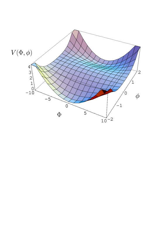
Figure 1: Artist’s view (not in scale) of the saddle point of the potential in Eq. (1).

Now, since the effective mass–squared of $\phi$ is

$$(m_{\phi}^{\rm eff})^{2}=\lambda\Phi^{2}-\alpha M^{2},$$ (4)

if $\Phi>\Phi_{c}$ then $\phi$ is driven to zero, where

$$\Phi_{c}\equiv\sqrt{\frac{\alpha}{\lambda}}\;M\sim\frac{m_{3/2}}{\sqrt{\lambda}}\,.$$ (5)

Suppose, therefore, that originally the system lies in the regime, where, $m_{3/2}<\Phi\leq m_{P}$ and $\phi\simeq 0$. With such initial conditions the effective potential for $\Phi$ becomes quadratic:

$$V(\Phi,\phi=0)=\frac{1}{2}m_{\Phi}^{2}\Phi^{2}+M_{S}^{4}.$$ (6)

Since, $\Phi<m_{P}$ we see that, when $\phi$ remains at the origin, the scalar potential is dominated by a false vacuum density corresponding to energy:

$$V_{\rm inf}^{1/4}\simeq M_{S}\;,$$ (7)

which results in a period of inflation. During this period, according to the Friedmann equation, we have $V_{\rm inf}^{1/4}\sim\sqrt{m_{P}H_{\rm inf}}$. In view of Eq. (7) this means that

$$H_{\rm inf}\sim m_{3/2}\;.$$ (8)

This is why there is no slow roll, because all the masses are of the order of the Hubble parameter during inflation, as expected by the action of supergravity corrections [5]. And yet, there is inflation as long as $\phi$ remains at (or very near) the origin.

Now, during this period the Klein-Gordon equation for $\Phi$ is

$$\ddot{\Phi}+3H_{\rm inf}\dot{\Phi}+m_{\Phi}^{2}\Phi=0\,,$$ (9)

where the dot denotes derivative with respect to the cosmic time $t$. The above has a solution of the form $\Phi\propto e^{\omega t}$, where

$$\omega=-\frac{3}{2}H_{\rm inf}\left[1\pm\sqrt{1-\frac{4}{9}\left(\frac{m_{\Phi}}{H_{\rm inf}}\right)^{2}}\;\right],$$ (10)

From Eq. (10) we see that the evolution of $\Phi$ depends on whether $m_{\Phi}$ is larger or not from $\frac{3}{2}H_{\rm inf}$. We look into both cases below.

2.1 Fast–Roll Inflation ($m_{\Phi}\leq\frac{3}{2}H_{\rm inf}$)

Fast-roll inflation was first introduced in Ref. [8]. It corresponds to a limited period of inflation possible when the mass of the inflaton is comparable to the Hubble parameter, as in our case. It turns out that, in our model, when $m_{\Phi}\mbox{\raisebox{-3.87495pt}{~{}$\stackrel{{\scriptstyle\mbox{$<$}}}{{\sim}}$~{}}}\frac{3}{2}H_{\rm inf}$, we end up with a period of fast-roll inflation, the details of which we will study in this section.

In this case, as suggested by Eq. (10), there are two exponential solutions to Eq. (9), both exponentially decreasing with time. The solution with the positive sign corresponds to the mode which decreases faster and rapidly disappears. Thus, the dominant solution is the one with the negative sign, which gives

$$\Phi=\Phi_{0}\exp(-F_{\Phi}\Delta N)\,,$$ (11)

where, $\Delta N=H_{\rm inf}\Delta t$ is the number of the elapsing e-foldings and

$$F_{\Phi}\equiv\frac{3}{2}\left(1-\sqrt{1-\frac{4}{3}|\eta_{\Phi}|}\right)<\frac{3}{2}\,,$$ (12)

with $\eta_{\Phi}$ being the slow–roll parameter defined as

$$\eta_{\Phi}\equiv\frac{m_{P}^{2}}{V}\frac{\partial^{2}V}{\partial\Phi^{2}} \Rightarrow |\eta_{\Phi}|\simeq\frac{m_{\Phi}^{2}}{3H_{\rm inf}^{2}}\mbox{\raisebox{-3.87495pt}{~{}$\stackrel{{\scriptstyle\mbox{$<$}}}{{\sim}}$~{}}}\frac{3}{4}\,,$$ (13)

where we used that $H_{\rm inf}^{2}\simeq V_{\rm inf}/3m_{P}^{2}$. The approximation that $H\simeq H_{\rm inf}=$ const. is justified for $\Phi_{c}<\Phi<m_{P}$ because

$$\epsilon\equiv-\frac{\dot{H}}{H^{2}}=\frac{\dot{\Phi}^{2}}{2m_{P}^{2}H^{2}}=\frac{1}{2}F_{\Phi}^{2}\left(\frac{\Phi}{m_{P}}\right)^{2}\ll 1\,,$$ (14)

where we have used Eq. (9) and also that $3(m_{P}H)^{2}=\frac{1}{2}\dot{\Phi}^{2}+V(\Phi)$ with $\dot{\Phi}=-F_{\Phi}H_{\rm inf}\Phi$, according to Eq. (11).

Therefore, in view of Eq. (11), we find that the total number of e-foldings corresponding to fast-roll inflation is given by

$$N_{\rm FR}=-\frac{1}{F_{\Phi}}\ln\left(\frac{\Phi_{\rm end}}{\Phi_{0}}\right)\simeq\frac{1}{F_{\Phi}}\ln\left(\frac{m_{P}}{m_{3/2}}\right)+\frac{1}{F_{\Phi}}\ln\sqrt{\lambda}\,,$$ (15)

where $\Phi_{0}\sim m_{P}$ and $\Phi_{\rm end}=\Phi_{c}\sim m_{3/2}/\sqrt{\lambda}$ are the initial and final values for the roll of $\Phi$ respectively [cf. Eq. (5)]. From the above it is evident that the larger $m_{\Phi}$ is the larger $F_{\Phi}$ is and, therefore, the smaller the number $N_{\rm FR}$ of the total e-foldings of Fast-Roll inflation. However, this number cannot become arbitrarily small because, if $m_{\Phi}$ is bigger than $\frac{3}{2}H_{\rm inf}$ then the dynamics of $\Phi$ becomes distinctly different. We explore this case in what follows.

2.2 Locked Inflation ($m_{\Phi}>\frac{3}{2}H_{\rm inf}$)

Locked inflation was introduced in Ref. [11], using a potential of the form shown in Eq. (1). This kind of inflation uses an inflaton field, which is oscillating on top of the false vacuum density responsible for inflation. It turns out that, in our model, in the case when $m_{\Phi}>\frac{3}{2}H_{\rm inf}$ we obtain this kind of behaviour for $\Phi$.

Indeed, in this case the Klein-Gordon Eq. (9) is solved by an equation of the form

$$\Phi=\bar{\Phi}(\Delta t)\,\cos(\omega_{\Phi}\Delta t)\,,$$ (16)

where

$$\omega_{\Phi}=H_{\rm inf}\sqrt{\left(\frac{m_{\Phi}}{H_{\rm inf}}\right)^{2}-\frac{9}{4}}\;\approx m_{\Phi}\sim m_{3/2}$$ (17)

and

$$\bar{\Phi}=\bar{\Phi}_{0}\exp\left(-\frac{3}{2}\,\Delta N\right)\,.$$ (18)

It may strike as odd that the field is oscillating instead of rolling toward the true minimum of the system. This is because, provided the frequency of the oscillations is large enough, the time that the oscillating field spends on top of the saddle point of the potential is too small to allow its escape from the oscillatory trajectory. Indeed, as shown in Eq. (17), the oscillation frequency is $\omega_{\Phi}\sim m_{\Phi}$ and the time interval that the field spends on top of the saddle point ($\Delta\Phi\leq\Phi_{c}$) is

$$\omega_{\Phi}\Delta t\sim\frac{\Delta\Phi}{\bar{\Phi}} \Rightarrow (\Delta t)_{\rm saddle}\sim\frac{\Phi_{c}}{m_{\Phi}\bar{\Phi}}\sim\frac{1}{\sqrt{\lambda}}\frac{1}{\bar{\Phi}}\,,$$ (19)

where $\bar{\Phi}$ is the amplitude of the oscillations. Originally this amplitude may be quite large $\bar{\Phi}\sim m_{P}$ but the expansion of the Universe dilutes the energy of the oscillations and, therefore, $\bar{\Phi}$ decreases, which means that $(\Delta t)_{\rm saddle}$ grows. However, until $(\Delta t)_{\rm saddle}$ becomes large enough to be comparable to the inverse of the tachyonic mass of $\phi$, the latter has no time to roll away from the saddle. Hence, the oscillations of $\Phi$ on top of the saddle continue until the amplitude decreases down to

$$\bar{\Phi}_{\rm end}\sim m_{3/2}/\sqrt{\lambda}\sim\Phi_{c}\;,$$ (20)

at which point $\phi$ departs from the origin and rolls down toward its vacuum expectation value (VEV) $M$. During the oscillations the density of the oscillating $\Phi$ is

$$\rho_{\Phi}=\frac{1}{2}\dot{\Phi}^{2}+\frac{1}{2}m_{\Phi}^{2}\Phi^{2}\simeq\frac{1}{2}m_{\Phi}^{2}\bar{\Phi}^{2}.$$ (21)

Comparing this with the overall potential density given in Eq. (6) we see that, for oscillation amplitude smaller than $m_{P}$, the overall density is dominated by the false vacuum density given in Eq. (7), which remains constant as long as $\phi$ remains locked at the origin. Hence, the Universe undergoes a period of inflation when $\bar{\Phi}$ lies in the region

$$\bar{\Phi}\in\left(m_{3/2}/\sqrt{\lambda},\;m_{P}\right)\,.$$ (22)

Therefore, in view of Eq. (18), the total number of e-foldings of locked inflation corresponds to the range shown in Eq. (22) and is given by

$$N_{\rm lock}=\frac{2}{3}\ln\left(\frac{m_{P}}{m_{3/2}}\right)+\frac{2}{3}\ln\sqrt{\lambda}\leq 24\,.$$ (23)

Figure 2: Plot of the number of e-foldings $N_{\Phi}$ (corresponding to inflation while $\phi\approx 0$) against the curvature of the potential along the direction of $\Phi$ (parameterised by the slow-roll parameter $\eta_{\Phi}$) near the transition point between fast-roll ($|\eta_{\Phi}|<3/4$) and locked ($|\eta_{\Phi}|\geq 3/2$) inflation. As shown $N_{\Phi}$ decreases with increasing $|\eta_{\Phi}|$ until the critical value $|\eta_{\Phi}|=3/2$ is reached, above which it remains constant; $N_{\Phi}=N_{\rm lock}$. For illustrative purposes, we have chosen $\lambda=1$.

From the above and in view also of Eqs. (12) and (15) we see that $N_{\rm FR}>N_{\rm lock}$. Hence, we have shown that $N_{\rm lock}$ is the minimum number of e-foldings that the Universe inflates while $\phi$ remains at (or very near) the origin. Thus, even though the slope for the rolling $\Phi$ field maybe arbitrarily steep, locked inflation guarantees that there are at least a fixed number of e-foldings of inflationary expansion. In Figure 2 we plot $N_{\Phi}$ in the neighbourhood of the transition between fast-roll and locked inflation.

However, from Eq. (23), we see that, for realistic values of the parameters, locked inflation alone cannot provide the necessary number of e-foldings corresponding to the cosmological scales. Fortunately, there is a subsequent period of inflation, this time driven by the scalar field $\phi$, after it departs from zero and rolls toward its VEV. This is another period of fast-roll inflation and we discuss it next.

3 Tachyonic Fast–Roll Inflation

In Ref. [8], fast-roll inflation corresponds to the roll of a field $\phi$ from a local maximum of its potential, when its tachyonic mass is comparable to the Hubble parameter, which is exactly the case for the $\phi$ field in our model. The $\phi$ field corresponds to the so–called waterfall field in regular hybrid inflation, which is thought to cause a phase transition that terminates inflation. However, in our case, inflation continues after the phase transition.

The tachyonic potential for $\phi$ is of the form [cf. Eq. (1)]

$$V(\phi)=V_{\rm inf}-\frac{1}{2}|(m_{\phi}^{\rm eff})^{2}|\phi^{2}+\frac{1}{4}\alpha\phi^{4},$$ (24)

where $V_{\rm inf}=M_{S}^{4}$ and $(m_{\phi}^{\rm eff})^{2}$ is given by Eq. (4). Since the roll of $\phi$ begins after $\bar{\Phi}<\Phi_{c}\sim m_{3/2}/\sqrt{\lambda}$, we see that $|(m_{\phi}^{\rm eff})^{2}|\sim m_{3/2}^{2}$ and also $(m_{\phi}^{\rm eff})^{2}\simeq-m_{\phi}^{2}$.

Now, the Klein-Gordon satisfied by $\phi$ is

$$\ddot{\phi}+3H_{\rm inf}\dot{\phi}-m_{\phi}^{2}\phi=0\,,$$ (25)

where $m_{\phi}\sim m_{3/2}$ as shown in Eq. (3). The above admits solutions of the form $\phi\propto\exp(\omega_{\phi}\Delta t)$ with

$$\omega_{\phi}=-\frac{3}{2}\;H_{\rm inf}\left[1\pm\sqrt{1+\frac{4}{9}\left(\frac{m_{\phi}}{H_{\rm inf}}\right)^{2}}\;\right]$$ (26)

The solution with the positive sign corresponds to the exponentially decreasing mode which rapidly disappears, whereas the solution with the negative sign corresponds to the exponentially growing mode:

$$\phi=\phi_{0}\exp(F_{\phi}\Delta N)\,,$$ (27)

where, $\Delta N=H_{\rm inf}\Delta t$ is the number of the elapsing e-foldings and

$$F_{\phi}\equiv\frac{3}{2}\left(\sqrt{1+\frac{4}{3}|\eta_{\phi}|}-1\right)\,,$$ (28)

with $\eta_{\phi}$ being the slow–roll parameter defined in a similar manner as in Eq. (13). For $\eta_{\phi}$ we have

$$|\eta_{\phi}|\equiv\frac{m_{P}^{2}}{V}\left|\frac{\partial^{2}V}{\partial\phi^{2}}\right|\simeq\frac{m_{\phi}^{2}}{3H_{\rm inf}^{2}}\sim 1\,,$$ (29)

The approximation that $H\simeq H_{\rm inf}=$ const. is again justified for $0<\phi<M\sim m_{P}$ because

$$\epsilon=\frac{1}{2}F_{\phi}^{2}\left(\frac{\phi}{m_{P}}\right)^{2}\ll 1\,,$$ (30)

where we have used Eq. (25) and also that $3(m_{P}H)^{2}=\frac{1}{2}\dot{\phi}^{2}+V(\phi)$ with $\dot{\phi}=F_{\phi}H_{\rm inf}\phi$ [cf. Eq. (27)].

Therefore, in view of Eq. (27), we find that the total number of e-foldings corresponding to fast-roll inflation is given by

$$N_{\phi}=\frac{1}{F_{\phi}}\ln\left(\frac{\phi_{\rm end}}{\phi_{0}}\right)\simeq\frac{1}{F_{\phi}}\ln\left(\frac{M}{m_{\phi}}\right)\,,$$ (31)

where $\phi_{0}$ and $\phi_{\rm end}$ are the initial and final values for the roll of $\phi$. The final value of $\phi$ is its VEV $M\sim m_{P}$, while the initial value of $\phi$ depends on the initial conditions at the onset of inflation (see Sec. 5.2.2 for a more detailed discussion on this issue). If $\phi$ is very close to the origin then $\phi_{0}$ is determined by the tachyonic fluctuations which send it off the top of the potential, and is given by $\phi_{0}=m_{\phi}/2\pi$ [18]. This is what we assume for the moment in Eq. (31).

From Eqs. (15), (23) and (31) we see that the total number of inflationary e-foldings is given by

$$N_{\rm tot}=N_{\Phi}+N_{\phi}\simeq\left(\frac{1}{\bar{F}_{\Phi}}+\frac{1}{F_{\phi}}\right)\ln\left(\frac{m_{P}}{m_{3/2}}\right)+\frac{1}{\bar{F}_{\Phi}}\ln\sqrt{\lambda}\,,$$ (32)

where we have set

$$\bar{F}_{\Phi}\equiv\min\left\{\frac{3}{2},\,F_{\Phi}\right\}\,$$ (33)

and $N_{\Phi}$ corresponds to the first stage of inflation and is given by [cf. Eqs. (15) and (23)]

$$N_{\Phi}=\simeq\frac{1}{\bar{F}_{\Phi}}\ln\left(\frac{m_{P}}{m_{3/2}}\right)+\frac{1}{\bar{F}_{\Phi}}\ln\sqrt{\lambda}\,,$$ (34)

It is the above number $N_{\rm tot}$, which needs to be compared to the necessary e-foldings for the cosmological scales.

4 The necessary e-foldings

Inflation solves in a single stroke the horizon and flatness problems of the Standard Hot Big Bang (SHBB) cosmology, while providing also the superhorizon spectrum of density perturbations necessary for the formation of Large Scale Structure. To do all these, the inflationary period has to be sufficiently long because the scales that correspond to the cosmological observations need to exit the horizon during inflation. The largest of these scales is determined by the requirements of the horizon problem and corresponds to about 100 times the scale of the present Horizon. The number of e-foldings required to inflate this scale on superhorizon size provides a lower bound on the total number of e-foldings of inflation and it is estimated as follows [4]:

$$N_{\rm cosmo}=72-\ln\left(\frac{m_{P}}{V_{\rm inf}^{1/4}}\right)-\frac{1}{3}\ln\left(\frac{V_{\rm inf}^{1/4}}{T_{\rm reh}}\right)-N_{0}\;,$$ (35)

where $V_{\rm inf}^{1/4}$ is the energy scale of inflation, $T_{\rm reh}$ is the reheat temperature, corresponding to the temperature of the thermal bath when the SHBB begins after the entropy production at the end of inflation, and $N_{0}\geq 0$ is the total e-foldings that correspond to any subsequent periods of inflation. The reheat temperature is given by

$$T_{\rm reh}\sim\sqrt{\Gamma m_{P}}\;,$$ (36)

where

$$\Gamma\simeq g^{2}m_{\phi}$$ (37)

is the decay rate for the inflaton field corresponding to the last stage of inflation and $g$ is the coupling of $\phi$ to the decay products. If the coupling of the field to other particles is extremely weak then the field will decay predominantly through gravitational couplings, in which case $\Gamma\sim m_{\phi}^{3}/m_{P}^{2}$. Thus, the effective range for $g$ is

$$\frac{m_{3/2}}{m_{P}}\leq g\leq 1\,,$$ (38)

where we considered that $m_{\phi}\sim m_{3/2}$.

Combining Eqs. (7), (36) and (37) we can recast Eq. (35) as

$$N_{\rm cosmo}=72-\frac{1}{2}\ln\left(\frac{m_{P}}{m_{3/2}}\right)+\frac{1}{3}\ln g-N_{0}\simeq 54-\frac{1}{3}\ln g-N_{0}$$ (39)

If our model is to explain the cosmological observations we have to demand that $N_{\rm tot}>N_{\rm cosmo}$. This provides an upper bound on $m_{\phi}$. Indeed, after a little algebra, it can be shown that Eqs. (32), (34) and (39), in view also of Eqs. (28) and (29), imply the bound

$$\frac{m_{\phi}}{H_{\rm inf}}<\frac{3}{2}\left\{\left[\left(\frac{108+\ln\sqrt{g}-\frac{3}{2\bar{F}_{\Phi}}\ln\sqrt{\lambda}-\frac{3}{2}N_{0}}{\ln(m_{P}/m_{3/2})}-\frac{3}{4}\left(1+\frac{2}{\bar{F}_{\Phi}}\right)\right)^{-1}+1\right]^{2}-1\right\}^{1/2},$$ (40)

which is more stringent the smaller $N_{\Phi}$ is. Thus, the tightest bound corresponds to a first stage of locked inflation, where $N_{\Phi}=N_{\rm lock}$ or, equivalently, when $\bar{F}_{\Phi}=3/2$. In this case the above bound becomes:

$$\frac{m_{\phi}}{H_{\rm inf}}<\frac{3}{2}\left\{\left[\left(\frac{108+\ln\sqrt{g/\lambda}-\frac{3}{2}N_{0}}{\ln(m_{P}/m_{3/2})}-\frac{7}{4}\right)^{-1}+1\right]^{2}-1\right\}^{1/2}$$ (41)

Clearly, the above suggest that the upper bound on $m_{\phi}/H_{\rm inf}$ is of order unity. For example, for the range given in Eq. (38) and if we choose $N_{0}=0$ and $\lambda\sim 1$ it is easy to show that the above bound interpolates between 2 and 3. Moreover, if the mass of $\Phi$ is below $\frac{3}{2}H_{\rm inf}$ then $N_{\Phi}=N_{\rm FR}\geq N_{\rm lock}$ and the bound on $m_{\phi}$ is further relaxed because $N_{\phi}$ does not need to be as large as before.

Consequently, it seems that, regardless of $m_{\Phi}$, the required e-foldings of inflation corresponding to the cosmological scales can be attained, only with a mild upper bound on $m_{\phi}$. However, there is one grave danger that we had overlooked and this is the possibility of disastrous Primordial Black Hole production due to the phase transition that terminates the first stage of inflation. We elaborate on this problem in the next section.

5 The danger from Primordial Black Hole production

A rather important issue to be investigated is the possibility of excessive Primordial Black Hole (PBH) production after the end of inflation, when the scale, which corresponds to the phase transition that releases $\phi$ from the top of the saddle, reenters the horizon.

5.1 The PBH calamity

It is well known that the outburst of tachyonic fluctuations at the phase transition can generate a mountain of density/curvature perturbations (localised around the scale corresponding to the phase transition) with amplitude of order unity [19]. When these perturbations reenter the horizon and become causally connected they can collapse and form PBHs [20]. The mass of these PBHs is of the order of the mass included in the horizon volume at the time of reentry, i.e.

$$M_{\sc pbh}\sim\left.\frac{\rho}{H^{3}}\right|_{\sc pbh}\sim\frac{m_{P}^{2}}{H_{\sc pbh}}\,,$$ (42)

where the subscript ‘pbh’ denotes the epoch of PBH formation. The probability of PBH formation is of order unity, which means that a sizable fraction of the energy density of the Universe collapses into PBHs and then scales as pressureless matter. Hence, just after their formation, the PBHs dominate the density of the Universe and result in a period of matter domination. This period lasts until the PBHs evaporate, which occurs after time $\Delta t_{\rm ev}$, where [21]

$$\Delta t_{\rm ev}\sim\frac{M_{\sc pbh}^{3}}{m_{P}^{4}}\;.$$ (43)

One of the greatest successes of the SHBB is the correct prediction for the delicate abundance of the light elements. They are generated during a process called Big Bag Nucleosynthesis (BBN), which takes place at temperatures $T_{\sc bbn}\sim 1$ MeV, at cosmic time of about 1 sec. The BBN process is very sensitive to the state of the Universe at the time. Consequently, it is imperative that the SHBB has begun before BBN occurs.

Therefore, the PBHs must evaporate before BBN, i.e. $\Delta t_{\rm ev}<H_{\sc bbn}^{-1}\sim 1$ sec. This requirement results in a constraint on $M_{\sc pbh}$, which reads

$$M_{\sc pbh}^{3}<\frac{m_{P}^{5}}{T_{\sc bbn}^{2}}\qquad\Rightarrow\qquad M_{\sc pbh}<10^{32}{\rm GeV}\sim 10^{8}{\rm g}\,.$$ (44)

To calculate the value of $M_{\sc pbh}$ we use the fact that the formation of the PBHs occurs when the scale that corresponds to the phase transition, reenters the horizon. Since this scale exits the horizon $N_{\phi}$ e-foldings before the end of inflation, it is easy to find

$$\frac{a_{\sc pbh}}{a_{\rm inf}}\sim\exp(N_{\phi})\sim\left(\frac{m_{P}}{m_{\phi}}\right)^{1/F_{\phi}},$$ (45)

where $a(t)$ is the scale factor of the Universe, the subscript ‘inf’ here denotes the end of inflation and we used Eq. (31). To proceed we need to consider individually the cases when the PBH formation takes place before and after reheating.

5.1.1 PBH formation before reheating ($H_{\sc pbh}\geq\Gamma$)

In this case the Universe after the end of inflation and until the formation of PBHs remains matter dominated so that $a\propto H^{-2/3}$. Then, Eq. (45) gives

$$H_{\sc pbh}\sim H_{\rm inf}\left(\frac{m_{P}}{m_{\phi}}\right)^{-3/2F_{\phi}}.$$ (46)

Substituting the above into Eq. (42) and considering also that $m_{\phi}\sim m_{3/2}\sim H_{\rm inf}$ we obtain

$$M_{\sc pbh}\sim m_{P}\left(\frac{m_{P}}{m_{3/2}}\right)^{\frac{3}{2F_{\phi}}+1}.$$ (47)

Enforcing in the above the bound in Eq. (44) we end up with the requirement

$$\left(\frac{m_{P}}{m_{3/2}}\right)^{\frac{9}{2F_{\phi}}+1}<\left(\frac{m_{3/2}}{T_{\sc bbn}}\right)^{2},$$ (48)

which is impossible to satisfy with $F_{\phi}\geq 0$.

Note that, if $F_{\phi}\gg 1$ then Eq. (48) can be recast as $V_{\rm inf}^{1/4}>m_{P}(T_{\sc bbn}/m_{P})^{1/3}$, where we used Eq. (7). Satisfying this bound is marginally viable but requires a huge value of $F_{\phi}$ or, equivalently, $m_{\phi}\gg H_{\rm inf}$, which eliminates the second stage of inflation.

5.1.2 PBH formation after reheating ($H_{\sc pbh}<\Gamma$)

In this case, after the end of inflation, the Universe is matter dominated ($a\propto H^{-2/3}$) until reheating, but afterwards and until PBH formation it becomes radiation dominated with $a\propto H^{-1/2}$. Therefore, Eq. (45) gives

$$H_{\sc pbh}\sim H_{\rm inf}\left(\frac{H_{\rm inf}}{\Gamma}\right)^{1/3}\left(\frac{m_{P}}{m_{\phi}}\right)^{-2/F_{\phi}}.$$ (49)

Substituting the above into Eq. (42) and considering also that $m_{\phi}\sim m_{3/2}\sim H_{\rm inf}$ we obtain

$$M_{\sc pbh}\sim g^{2/3}m_{P}\left(\frac{m_{P}}{m_{3/2}}\right)^{\frac{2}{F_{\phi}}+1},$$ (50)

where we also used Eq. (37). Enforcing in the above the bound in Eq. (44) we end up with the requirement

$$g^{2}\left(\frac{m_{P}}{m_{3/2}}\right)^{\frac{6}{F_{\phi}}+1}<\left(\frac{m_{3/2}}{T_{\sc bbn}}\right)^{2}.$$ (51)

Now, it is evident that Eq. (49) can be recast as

$$\frac{H_{\sc pbh}}{\Gamma}\sim g^{-8/3}\left(\frac{m_{P}}{m_{3/2}}\right)^{-2/F_{\phi}}.$$ (52)

Enforcing into the above the bound in Eq. (51) and taking also into account that $H_{\sc pbh}<\Gamma$ it is easy to show that we end up again with Eq. (48).

Therefore, it seems that, in our model, PBH production unavoidably disturbs BBN, since it turns out that the PBHs cannot evaporate early enough. This disappointing result has been reached numerically also in Ref. [14]. The only escape from this catastrophe is to avoid producing any PBHs in the first place. In contrast to Ref. [14], we show that there is ample parameter space where this can be achieved in a natural way. The key to the solution is to avoid fixing $\phi\simeq 0$ as the initial condition for $\phi$. Indeed, in the following section we elaborate on this issue and consider a more realistic initial value for $\phi$, which, for small enough $\lambda$, results in no PBH production.

5.2 The solution to the PBH problem

5.2.1 A way out

One can avoid the generation of PBHs if, at the time when the amplitude of the oscillating $\Phi$ is decreased down to $\Phi_{c}$, the field $\phi$ is significantly displaced from the top of the saddle so that the tachyonic fluctuations are suppressed. Hence, we require that $\phi_{0}>m_{\phi}$. Writing

$$\phi_{0}\equiv\beta m_{\phi}\;,$$ (53)

to avoid PBH production we need

$$1\ll\beta\ll\frac{M}{m_{\phi}}\sim 10^{15}\,,$$ (54)

where the upper bound ensures the ‘locking’ of $\phi$ on top of the saddle. In view of the above, Eq. (31) becomes

$$N_{\phi}\simeq\frac{1}{F_{\phi}}\ln\left(\frac{M}{m_{\phi}}\right)-\frac{1}{F_{\phi}}\ln\beta$$ (55)

Using this we can reproduce the bound in Eq. (40), which now becomes

$$\frac{m_{\phi}}{H_{\rm inf}} < \frac{3}{2}\left\{\left[\left(\frac{108+\ln\sqrt{g}-\frac{3}{2\bar{F}_{\Phi}}\ln\sqrt{\lambda}-\frac{3}{2}N_{0}}{\ln(m_{P}/m_{3/2})}-\frac{3}{4}\left(1+\frac{2}{\bar{F}_{\Phi}}\right)\right)^{-1}\right.\right.\times$$ (56)

$$\times\left.\left.\left(1-\frac{\ln\beta}{\ln(m_{P}/m_{3/2})}\right)+1\right]^{2}-1\right\}^{1/2},$$

where, from Eq. (54), it is evident that

$$0<\frac{\ln\beta}{\ln(m_{P}/m_{3/2})}<1\,.$$ (57)

Thus, we see that the upper bound on the tachyonic mass of the $\phi$ modulus is somewhat strengthened.

5.2.2 The initial value of $\phi$ at the phase transition

To obtain an estimate of the likely value of $\beta$ we have to take a closer look on the evolution of $\phi$ during the first period of inflation, when $\bar{\Phi}\gg\Phi_{c}$. Then we can write the Klein-Gordon equation of $\phi$ as

$$\dot{\phi}\ddot{\phi}+3H_{\rm inf}\dot{\phi}^{2}+V^{\prime}(\phi)\dot{\phi}=0\,,$$ (58)

where the prime here denotes derivative with respect to $\phi$ and we have multiplied the Klein-Gordon with $\dot{\phi}$. Now, when $\bar{\Phi}>\Phi_{c}$ we have $(m_{\phi}^{\rm eff})^{2}\simeq\lambda\Phi^{2}$ and $V(\phi)\simeq\frac{1}{2}\lambda\Phi^{2}\phi^{2}$. Using this it is easy to show that

$$V^{\prime}(\phi)\dot{\phi}=\dot{V}(\phi)-2V(\phi)(\dot{\Phi}/\Phi)\simeq\dot{V}(\phi)+3H_{\rm inf}V(\phi)\,,$$ (59)

where we have approximated $\Phi\sim\bar{\Phi}$ (which holds during almost the entire oscillation period of $\Phi$) and considered that [cf. Eq. (21)] $\rho_{\Phi}\propto\bar{\Phi}^{2}\propto\exp(-3H_{\rm inf}t)$, which results in $\dot{\Phi}/\Phi\sim-\frac{3}{2}H_{\rm inf}$.

Using the above, Eq. (58) can be written as

$$\dot{\rho}_{\phi}+3H_{\rm inf}[2\rho_{\phi}^{\rm kin}+V(\phi)]=0\,,$$ (60)

where the kinetic density of $\phi$ is $\rho_{\phi}^{\rm kin}\equiv\frac{1}{2}\dot{\phi}^{2}$ and $\rho_{\phi}=\rho_{\phi}^{\rm kin}+V(\phi)$. Now, since during the first period of inflation we have $(m_{\phi}^{\rm eff})^{2}\sim\lambda\bar{\Phi}^{2}\gg\lambda\Phi_{c}^{2}\sim H_{\rm inf}$, during a Hubble time $\phi$ undergoes a huge number of oscillations. This means that these oscillations are, to a very good approximation, harmonic. Consequently, following the reasoning of [23] (see also [3]), we can consider $\bar{\rho}_{\phi}^{\rm kin}\simeq\bar{V}(\phi)\simeq\frac{1}{2}\rho_{\phi}$, where the bar here means “average per oscillation”. Hence, Eq. (60) can be recast as

$$\dot{\rho}_{\phi}+\frac{9}{2}H_{\rm inf}\rho_{\phi}\simeq 0\,.$$ (61)

This means that $\rho_{\phi}\simeq 2\bar{V}(\phi)\propto\bar{\Phi}^{2}\bar{\phi}^{2}\propto\exp(-\frac{9}{2}H_{\rm inf}t)$. Hence, we see that $\rho_{\phi}/\rho_{\Phi}\propto\exp(-\frac{3}{2}H_{\rm inf}t)$, which means that the evolution of $\phi$ cannot influence the dynamics of the first stage of inflation (because soon after the onset of inflation $\rho_{\phi}$ becomes negligible compared to $\rho_{\Phi}$).

Now, considering that $\bar{\Phi}^{2}\propto\exp(-3H_{\rm inf}t)$ we see that $\bar{\phi}\propto\exp(-\frac{3}{4}H_{\rm inf}t)$. Hence, for the typical value of $\phi$ at the end of the first stage of inflation we have found

$$\phi_{0}\sim\bar{\phi}_{0}\sim\phi_{\rm in}\,\exp\left(-\frac{3}{4}N_{\Phi}\right)$$ (62)

where $\phi_{\rm in}$ is the initial value at the onset of inflation.

One might think that a natural value for $\phi_{\rm in}$ is $m_{P}$, since we are dealing with a modulus field. However, such a value would be possible only if the interaction term in the potential in Eq. (1) is not larger than $V_{\rm inf}$. Hence, using that $\Phi_{0}\sim m_{P}$ we find

$$\lambda\,\phi_{\rm in}^{2}\Phi_{0}^{2}\mbox{\raisebox{-3.87495pt}{~{}$\stackrel{{\scriptstyle\mbox{$<$}}}{{\sim}}$~{}}}V_{\rm inf}\quad\Rightarrow\quad\phi_{\rm in}\mbox{\raisebox{-3.87495pt}{~{}$\stackrel{{\scriptstyle\mbox{$<$}}}{{\sim}}$~{}}}\min\left\{\frac{m_{3/2}}{\sqrt{\lambda}},\;m_{P}\right\},$$ (63)

where we also used Eq. (7). Unless the initial conditions for $\phi$ are tuned to be very close to the origin, we expect the above bound to be saturated.

Now, from Eq. (34) it is evident that, for $N_{\Phi}>0$, we require

$$\lambda>\left(\frac{m_{3/2}}{m_{P}}\right)^{2}\sim 10^{-30}.$$ (64)

Hence, Eq. (63) suggests that

$$\phi_{\rm in}\sim\frac{m_{3/2}}{\sqrt{\lambda}}.$$ (65)

Therefore, using Eqs. (15), (34), (53), (62) and (65) we obtain:

$$\ln\beta\simeq-\frac{3}{4}N_{\Phi}-\ln\sqrt{\lambda}\simeq-\left(1+\frac{3}{4\bar{F}_{\Phi}}\right)\ln\sqrt{\lambda}-\frac{3}{4\bar{F}_{\Phi}}\ln\left(\frac{m_{P}}{m_{3/2}}\right).$$ (66)

5.2.3 The new bound on $m_{\phi}$

Incorporating Eq. (66) into Eq. (56), the bound on $m_{\phi}$ is recast as

$$\frac{m_{\phi}}{H_{\rm inf}} < \frac{3}{2}\left\{\left[\left(\frac{108+\ln\sqrt{g}-\frac{3}{2}N_{0}}{\ln(m_{P}/m_{3/2})}-\frac{3}{4}-\frac{3}{2\bar{F}_{\Phi}}\left(1+\frac{\ln\sqrt{\lambda}}{\ln(m_{P}/m_{3/2})}\right)\right)^{-1}\times\right.\right.$$ (67)

$$\times\left.\left.\left(1+\frac{3}{4\bar{F}_{\Phi}}\right)\left(1+\frac{\ln\sqrt{\lambda}}{\ln(m_{P}/m_{3/2})}\right)+1\right]^{2}-1\right\}^{1/2}.$$

Moreover, inserting Eq. (66) into Eq. (57) we find

$$-\ln\left(\frac{m_{P}}{m_{3/2}}\right)<\ln\sqrt{\lambda}<-\left(1+\frac{4}{3}\bar{F}_{\Phi}\right)^{-1}\ln\left(\frac{m_{P}}{m_{3/2}}\right)\leq-\frac{1}{3}\ln\left(\frac{m_{P}}{m_{3/2}}\right),$$ (68)

which is consistent with the bound in Eq. (64) and for the last inequality we used Eq. (33). Note that the upper bound in the above demands $\lambda\leq 10^{-10}$.

The upper bound in Eq. (68) results in a lower bound on $m_{\Phi}$. It is easy to see that this bound, for a given $\lambda$, reads

$$\frac{m_{\Phi}}{H_{\rm inf}}>\frac{3}{2}\left[1-\frac{1}{4}\left(3+\frac{\ln(m_{P}/m_{3/2})}{\ln\sqrt{\lambda}}\right)^{2}\right]^{1/2}.$$ (69)

If $m_{\Phi}$ were smaller than the above bound then $N_{\Phi}$ would be too large, which would allow enough time for $\bar{\phi}$ to decrease below $m_{\phi}$ by the time of the phase transition, resulting into copious PBH production.

5.2.4 Example case: $\lambda\sim\sqrt{\alpha}$

To illustrate the above somewhat clearer let us choose

$$\lambda\sim\sqrt{\alpha}\sim\frac{m_{3/2}}{m_{P}}\sim 10^{-15}$$ (70)

We immediately see that, according to Eq. (69), the bound on $m_{\Phi}$ is

$$\frac{m_{\Phi}}{H_{\rm inf}}>\frac{3\sqrt{3}}{4}\approx 1.3\;,$$ (71)

which corresponds to

$$\frac{3}{4}<\bar{F}_{\Phi}\leq\frac{3}{2}$$ (72)

As far as the bound on $m_{\phi}$ is concerned, it is straightforward to show that Eq. (67) becomes

$$\frac{m_{\phi}}{H_{\rm inf}}<\frac{3}{2}\left\{\left[\left(\frac{108+\ln\sqrt{g}-\frac{3}{2}N_{0}}{\ln(m_{P}/m_{3/2})}-\frac{3}{4}\left(1+\frac{1}{\bar{F}_{\Phi}}\right)\right)^{-1}\frac{1}{2}\left(1+\frac{3}{4\bar{F}_{\Phi}}\right)+1\right]^{2}-1\right\}^{1/2},$$ (73)

while Eq. (66) gives

$$\ln\beta\simeq\frac{1}{2}\left(1-\frac{3}{4\bar{F}_{\Phi}}\right)\ln\left(\frac{m_{P}}{m_{3/2}}\right)>0,$$ (74)

where we also used Eq. (72).

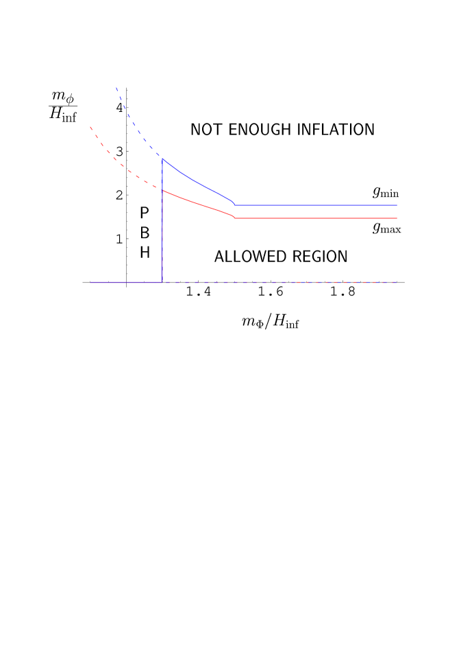
Figure 3: Plot of the allowed parameter space for the masses of the moduli $\Phi$ and $\phi$ in order for hybrid inflation without flat directions to work, in the case when $\lambda\sim\sqrt{\alpha}$ and $N_{0}=0$. The solid lines denote the borders of the allowed region. In particular, the upper {lower} line corresponds to the minimum {maximum} value of $g$, i.e. $g_{\rm min}\sim m_{3/2}/m_{P}$ {$g_{\rm max}\sim 1$} according to Eq. (38). The region above the border lines is excluded because $m_{\phi}$ is too large to allow an adequately long tachyonic fast-roll inflation phase . Hence, this region corresponds to inflation with not enough e-foldings to explain the cosmological observations (i.e. solve the flatness and horizon problems). The region on the left of the the border line is excluded because $m_{\Phi}$ is small enough to result in a long first stage of fast-roll inflation, which enables $\phi$ to roll too much toward the origin. Hence, in this region, the tachyonic fluctuations at the end of the first stage of inflation dominate the motion of $\phi$ and result in cosmologically catastrophic production of Primordial Black Holes (PBHs). The two forbidden regions are separated by a dashed line, whose position depends again on the value of $g$. The distinction between a first stage of fast roll or locked inflation is evident. For $m_{\Phi}>\frac{3}{2}H_{\rm inf}$ we have locked inflation, in which case the upper bound on $m_{\phi}$ is independent of $m_{\Phi}$ [cf. Eq. (75)]. This bound is relaxed for smaller $m_{\Phi}$, when we have a first stage of fast roll inflation. Avoiding PBH production bounds $m_{\Phi}$ from below as $m_{\Phi}>1.3\,H_{\rm inf}$, according to Eq. (71). We see that the allowed parameter space corresponds to $m_{\phi}\sim m_{\Phi}\sim H_{\rm inf}$ as required.

If we further set $m_{\Phi}>\frac{3}{2}H_{\rm inf}$, then the first stage of inflation corresponds to locked inflation and $\bar{F}_{\Phi}=3/2$. In this case Eq. (73) becomes

$$\frac{m_{\phi}}{H_{\rm inf}}<\frac{3}{2}\left\{\left[\left(\frac{72+\frac{2}{3}\ln\sqrt{g}-N_{0}}{\ln(m_{P}/m_{3/2})}-\frac{5}{4}\right)^{-1}\frac{1}{2}+1\right]^{2}-1\right\}^{1/2},$$ (75)

which, for $N_{0}=0$ and for the range of $g$ in Eq. (38), interpolates between between 1.5 and 1.8. Hence, it is evident that enough inflation to satisfy the cosmological observations can be achieved with

$$m_{\Phi}\sim m_{\phi}\sim m_{3/2}\sim H_{\rm inf}\;,$$ (76)

i.e. without the use of a flat direction. Hence, we have shown that the combination of locked and fast-roll inflation is capable of providing enough e-foldings of inflation to encompass the cosmological scales without the use of any flat direction. Note that the bound in Eq. (75) is further relaxed if $m_{\Phi}<\frac{3}{2}H_{\rm inf}$ as can be seen in Figure 3.

Now, regarding the catastrophic possibility of PBH production, Eq. (74), in the case when $m_{\Phi}\geq\frac{3}{2}H_{\rm inf}$, gives

$$\ln\beta\simeq 8.64\Rightarrow\beta\sim 6\times 10^{3},$$ (77)

which means that $\phi$ is always safely away from the origin so that the tachyonic fluctuations never dominate its motion and, consequently, there is no excessive production of perturbations and no PBH formation. If $m_{\Phi}<\frac{3}{2}H_{\rm inf}$, then $\bar{F}_{\Phi}<3/2$ and $\beta$ is reduced, but, as shown in Eq. (74), it is always greater than unity.

In total we have shown that there is ample parameter space in which PBH production is avoided while enough inflation is achieved without the use of flat directions. However, there are more requirements to be met for a successful cosmology. We discuss the most important of them in the following section.

6 Other cosmological considerations

6.1 Curvature perturbations

There are more to inflation than the solution of the horizon and flatness problems. In particular inflation has to provide also the spectrum of superhorizon density/curvature perturbations which causes the observed CMBR anisotropy and seeds the formation of Large Scale Structure in the Universe. The superhorizon spectrum of perturbations is thought to be generated by the amplification of the quantum fluctuations of a light field, i.e. a field whose mass is smaller than $H_{\rm inf}$. This is because only if the Compton wavelength of the field is larger than the horizon during inflation, can the quantum fluctuations of the field reach and exit the horizon, thereby giving rise to the desired generation of a superhorizon perturbation spectrum. This is a rather generic requirement, which seems to call for the use of at least one flat direction in inflation.

Traditionally, it was thought that the field responsible for the generation of the superhorizon curvature perturbations is the inflaton field. However, this is possible only if the inflaton is effectively massless, i.e. only if $m_{\Phi}\ll H_{\rm inf}$. This is in conflict with our aim in this paper, which is to achieve inflation without the use of flat directions, which means that, for our inflaton, $m_{\Phi}\sim H_{\rm inf}$. Consequently an alternative solution must be found.

There are a number of recent proposals on this issue in the literature. For example, in Ref. [11] it is assumed that $\phi$ is coupled to some other field $\chi$ in a way, which does not affect the inflationary scenario but does affect the inflaton decay rate $\Gamma$. The latter is thought to be perturbed on superhorizon scales because $\chi$ is assumed to be an appropriately light field. This mechanism was recently introduced in Ref. [24] and, even though quite interesting, it suffers from the fact that we require our moduli inflatons to possess the appropriate coupling to the appropriate field, which should be large enough to generate the required perturbations but not too large because it should not lift the flatness of the $\chi$ direction. It seems, therefore, that this mechanism needs a few special requirements to work. This is against our philosophy, which aims to address the problems of inflation model–building in the most generic and natural way possible.

Fortunately there is another way to obtain the required curvature perturbations. Recently it has been suggested that the generation of these superhorizon perturbations could be entirely independent of the inflaton field. Indeed, according to this proposal the curvature perturbation spectrum is due to the superhorizon perturbations of some “curvaton” field $\sigma$ [15]. As usual, this field must be a light field during inflation. Its energy density during inflation is negligible and, therefore, has no effect on the inflationary dynamics. After the end of inflation, however, the field becomes important and manages to dominate (or nearly dominate) the energy density, imposing thereby its own curvature perturbation onto the Universe. Afterwards, it decays into the thermal bath of the SHBB.

The existence of a curvaton field substantially ameliorates the constraints imposed by observations onto inflation model-building [10]. Indeed, the only requirement that the curvaton imposes onto inflation is that the inflaton itself does not generate excessive curvature perturbations. In our case, though, there is no such danger because our inflatons are not light fields and, therefore, they do not produce any sizable superhorizon curvature perturbations, because their quantum fluctuations are exponentially suppressed before reaching the horizon during inflation.

The curvaton is generally expected to produce a quite flat superhorizon spectrum of curvature perturbations, which is in good agreement with the recent WMAP observations that suggest $n_{s}\approx 1$ for the spectral index. However, the predictions of the curvaton depend on the evolution of the field after the end of inflation, which has been thoroughly investigated in a recent paper of one of us, with collaborators [25]. In particular, if the curvaton decays before it dominates the Universe it may generate a substantial isocurvature component on the perturbation spectrum, correlated with the adiabatic mode, which may soon become observable by the Planck satellite. Also, it is possible to obtain sizable non-Gaussianity that may be constrained or detected by the SDSS or the 2dF galaxy surveys [15].

The advantage of the curvaton is that, since it is independent of the physics of inflation, it can be associated with much lower energy scales than $V_{\rm inf}^{1/4}$. In particular, it may well be associated with TeV physics, and can be a field already present in simple extensions of the Standard Model. Indeed, physics beyond the Standard Model provides a large number of curvaton candidates such as, a right-handed sneutrino [26], used for generating the neutrino masses, the Peccei-Quinn field [27], which solves the strong CP problem, various flat directions of the MSSM [28], or of the NMSSM [29], a PNGB [30] (e.g. a Wilson line or a string axion) and a string modulus [31] to name but some.

6.2 The moduli problem

The fact that the SHBB must have already begun before BBN takes place sets a lower bound on $T_{\rm reh}$ for any inflationary model. This bound translates into a bound on $\Gamma$ [cf. Eq. (36)] which, in turn, becomes a bound on $g$ of Eq. (37). Indeed, demanding $\Gamma\gg H_{\sc bbn}\sim 10^{-24}$ GeV, we find that BBN constrains $g$ as follows:

$$g\geq 10\;\frac{m_{3/2}}{m_{P}}\,.$$ (78)

Thus, we see that almost the entire range in Eq. (22) escapes the above bound. There is a problem only if $\phi$ decays through gravitational couplings, in which case $\Gamma\sim m_{3/2}^{3}/m_{P}^{2}$. This is the well known moduli problem. A typical solution to this problem involves the introduction of an additional brief period of thermal inflation [9], which dilutes the moduli and produces additional entropy, which enables the SHBB to commence earlier than BBN. This period of thermal inflation may occur during the inflaton’s coherent oscillations, before reheating is completed.

Typically, thermal inflation may last up to 20 e-foldings. This means that, in Eq. (39), the term $N_{0}$ would be non zero, but equal to the number of e-foldings of thermal inflation. When $N_{0}>0$ the upper bound on $m_{\phi}$ in Eq. (67) is relaxed. For example, with $\lambda\sim\sqrt{\alpha}$ and $m_{\Phi}>\frac{3}{2}H_{\rm inf}$, putting $N_{0}=10$ {$N_{0}=14$} relaxes the bound on the ratio of $m_{\phi}/H_{\rm inf}$ [cf. Eq. (75)] up to 5 {9}. For $N_{0}\rightarrow 17.3$ it can be shown that there is no need for a second stage of fast-roll inflation and $m_{\phi}$ can be very large as shown in Figure 4.

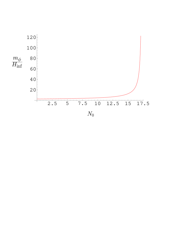
Figure 4: Plot of the upper bound on the ratio $m_{\phi}/H_{\rm inf}$ with respect to $N_{0}$ (the number of e-foldings corresponding to a brief period of thermal inflation, invoked to overcome the moduli problem), in the case when $\lambda\sim\sqrt{\alpha}$ and $\phi$ decays gravitationally, i.e. when $g\sim m_{3/2}/m_{P}$. We see that the larger $N_{0}$ is the weaker the bound becomes. When $N_{0}\rightarrow 17.3$ there is no need for any tachyonic, fast-roll inflation and $m_{\phi}$ can be arbitrarily large.

7 Discussion and conclusions

Using a rather generic form for their scalar potential, we have shown that moduli fields, corresponding to flat directions of supersymmetry, whose flatness is lifted by supergravity corrections, can naturally generate enough e-foldings of inflation to solve the horizon and the flatness problems of the Standard Hot Big Bang (SHBB). Indeed, using natural values for the parameters (masses of order TeV and vacuum energy of the order of the intermediate scale, corresponding to gravity mediated supersymmetry breaking) and a hybrid-type potential we have found that the moduli give rise to two-stage inflation whose total duration may well be long enough to encompass the cosmological scales. Depending on the curvature of the potential the first stage of inflation may be a period of fast-roll inflation or of oscillatory inflation, when the system is ‘locked’ on top of an unstable saddle point corresponding to non-zero vacuum density. This is followed by a second stage of tachyonic fast-roll inflation, when the system rolls toward the true vacuum. Our calculations have demonstrated that, with a quite mild upper bound on the tachyonic mass of the inflaton, we can achieve enough e-foldings of inflation without employing slow roll at all. That way inflation can escape from the famous $\eta$-problem, since we manage to have masses of order the Hubble parameter without problem.

Probably the most difficult obstacle to the success of our scenario is the possibility of copious generation of of Primordial Black Holes (PBHs). They may be generated due to excessive tachyonic fluctuations at the phase transition, which terminates the first stage of inflation. We have studied this problem in detail and showed that, if the PBHs do form then it is impossible to return to the SHBB cosmology in time for BBN. The only solution is, therefore, to avoid creating the PBHs in the first place. By considering the initial conditions of $\phi$ more carefully and by following its evolution during the first stage of inflation we have demonstrated that it is indeed possible to prevent it from being, at the time of the phase transition, under the influence of excessive tachyonic fluctuations, which would lead to PBH production. Instead, we have shown that, with natural initial conditions, one can avoid the PBHs provided $\lambda$ is not very large ($\lambda\sim 10^{-10}$ at most), i.e. the interaction between the moduli is suppressed. This is quite likely for moduli fields away from enhanced symmetry points (especially if the coupling is controlled by the Planck–suppressed VEV of some other field). Note, also, that avoiding the PBHs in the way we propose also dispenses with another potential danger; that of generating cosmologically catastrophic topological defects at the phase transition. For example, were it otherwise, it would be possible to generate stable domain walls, which would disastrously dominate the Universe. Still, one can consider more complicated theories where such defects are unstable or harmless (e.g. cosmic strings at the energy scale $M_{S}$ have little cosmological consequences).

Structure formation, in our model, is due to the existence of a curvaton field, which is unrelated to the moduli inflatons and, consequently, it can neither affect the dynamics of inflation nor does it have to be tuned accordingly to avoid this danger. The curvaton must be a flat direction because there is no known way to obtain the superhorizon spectrum of density perturbations required by the observations, other than inflating the vacuum fluctuations of a light scalar field. However, since the curvaton is not related with the inflationary expansion, it can be protected by some symmetry, which may even be exact during inflation (e.g. a global U(1) for a PNGB curvaton). Moreover, the curvaton can be associated with low energy (TeV) physics and can be easily accommodated in simple extensions of the Standard Model.

As discussed also in Ref. [11] the potential landscape for the moduli fields is expected to allow a cascade of periods of oscillatory, ‘locked’ inflation. Completing this picture we add that, between those periods, we can easily have periods of fast-roll inflation when the system is rolling from one saddle point to another. That way the total number of e-foldings can be much larger than the one corresponding to the cosmological scales. Of course one needs a roughly flat region of the Universe to start up with, but this is a generic initial condition problem for inflation. This work shows that, at least, the other generic problem of inflation, namely the $\eta$-problem, can be naturally overcome.

Acknowledgements: We would like to thank David H. Lyth for discussion and comments.

References

- [1] D. N. Spergel et al., Astrophys. J. Suppl. 148 (2003) 175; H. V. Peiris et al., Astrophys. J. Suppl. 148 (2003) 213; E. Komatsu et al., Astrophys. J. Suppl. 148 (2003) 119; http://map.gsfc.nasa.gov/.
- [2] A. Linde, “Particle Physics and Inflationary Cosmology”, Harwood 1990.
- [3] E. W. Kolb and M S. Turner, “The Early Universe”, Addison-Wesley, Reading MA, 1990.
- [4] A. R. Liddle and D. H. Lyth, “Cosmological Inflation and Large Scale Structure”, Cambridge University Press, Cambridge U.K., 2000; D. H. Lyth and A. Riotto, Phys. Rept. 314 (1999) 1.
- [5] M. Dine, L. Randall and S. Thomas, Nucl. Phys. B 458 (1996) 291; Phys. Rev. Lett. 75 (1995) 398.
- [6] E. Komatsu et al., Astrophys. J. Suppl. 148 (2003) 119; A. B. Lahanas and D. V. Nanopoulos, Phys. Rept. 145 (1987) 1.
- [7] K. Freese, J. A. Frieman and A. V. Olinto, Phys. Rev. Lett. 65 (1990) 3233; K. Freese, J. A. Frieman and A. V. Olinto, Phys. Rev. Lett. 65 (1990) 3233.
- [8] A. Linde, JHEP 0111 (2001) 052.
- [9] D. H. Lyth and E. D. Stewart, Phys. Rev. D 53 (1996) 1784; Phys. Rev. Lett. 75 (1995) 201.
- [10] K. Dimopoulos and D. H. Lyth, Phys. Rev. D 69 (2004) 123509.
- [11] G. Dvali and S. Kachru, hep-th/0309095; hep-ph/0310244.
- [12] A. D. Linde, Phys. Rev. D 49 (1994) 748.
- [13] A. H. Guth, Phys. Rev. D 23 (1981) 347; A. H. Guth and E. J. Weinberg, Nucl. Phys. B 212 (1983) 321.
- [14] R. Easther, J. Khoury and K. Schalm, JCAP 0406 (2004) 006.
- [15] D. H. Lyth and D. Wands, Phys. Lett. B 524 (2002) 5; D. H. Lyth, C. Ungarelli and D. Wands, Phys. Rev. D 67 (2003) 023503.
- [16] T. Damour and V. F. Mukhanov, Phys. Rev. Lett. 80 (1998) 3440; A. R. Liddle and A. Mazumdar, Phys. Rev. D 58 (1998) 083508; V. Cardenas and G. Palma, Phys. Rev. D 61 (2000) 027302; M. Sami, Grav. Cosmol. 8 (2003) 309.
- [17] A. Mazumdar, hep-th/0310162.
- [18] G. N. Felder, J. Garcia-Bellido, P. B. Greene, L. Kofman, A. D. Linde and I. Tkachev, Phys. Rev. Lett. 87 (2001) 011601; G. N. Felder, L. Kofman and A. D. Linde, Phys. Rev. D 64 (2001) 123517.
- [19] L. A. Kofman and A. D. Linde, Nucl. Phys. B 282 (1987) 555; L. A. Kofman and D. Y. Pogosian, Phys. Lett. B 214 (1988) 508.
- [20] B. J. Carr and S. W. Hawking, Mon. Not. Roy. Astron. Soc. 168 (1974) 399; B. J. Carr, Astrophys. J. 201 (1975) 1; A. G. Polnarev and M. Y. Khlopov, Sov. Phys. Usp. 28 (1985) 213 [Usp. Fiz. Nauk 145 (1985) 369].
- [21] S. W. Hawking, Nature 248 (1974) 30.
- [22] L. Kofman, A. D. Linde and A. A. Starobinsky, Phys. Rev. D 56 (1997) 3258.
- [23] M. S. Turner, Phys. Rev. D 28 (1983) 1243.
- [24] G. Dvali, A. Gruzinov and M. Zaldarriaga, Phys. Rev. D 69 (2004) 083505; Phys. Rev. D 69 (2004) 023505; L. Kofman, astro-ph/0303614; K. Enqvist, A. Mazumdar and M. Postma, Phys. Rev. D 67, 121303 (2003).
- [25] K. Dimopoulos, G. Lazarides, D. Lyth and R. Ruiz de Austri, Phys. Rev. D 68 (2003) 123515.
- [26] A. Hebecker, J. March-Russell and T. Yanagida, Phys. Lett. B 552 (2003) 229; J. McDonald, Phys. Rev. D 68 (2003) 043505; M. Postma and A. Mazumdar, JCAP 0401 (2004) 005; K. Hamaguchi, M. Kawasaki, T. Moroi and F. Takahashi, Phys. Rev. D 69 (2004) 063504.
- [27] K. Dimopoulos, G. Lazarides, D. Lyth and R. Ruiz de Austri, JHEP 0305 (2003) 057.
- [28] K. Enqvist, S. Kasuya and A. Mazumdar, Phys. Rev. Lett. 90, 091302 (2003); M. Postma, Phys. Rev. D 67, 063518 (2003); K. Enqvist, A. Jokinen, S. Kasuya and A. Mazumdar, hep-ph/0303165; S. Kasuya, M. Kawasaki and F. Takahashi, Phys. Lett. B 578 (2004) 259.
- [29] M. Bastero-Gil, V. Di Clemente and S. F. King, Phys. Rev. D 67 (2003) 103516; Phys. Rev. D 67, 083504 (2003).
- [30] K. Dimopoulos, D. H. Lyth, A. Notari and A. Riotto, JHEP 0307 (2003) 053; R. Hofmann, hep-ph/0208267; E. J. Chun, K. Dimopoulos and D. Lyth, hep-ph/0402059.
- [31] T. Moroi and T. Takahashi, Phys. Rev. D 66 (2002) 063501; Phys. Lett. B 522, 215 (2001).