The QCD vacuum, confinement and strings

in the Vacuum Correlator Method
D.S.Kuzmenko, V.I.Shevchenko, Yu.A.Simonov

Institute of Theoretical and Experimental Physics,
Moscow, Russia

e-mail: kuzmenko@heron.itep.ru; shevchen@heron.itep.ru; simonov@heron.itep.ru

In this review paper the QCD vacuum properties and the structure of color fields in hadrons are studied using complete set of gauge-invariant correlators of the gluon fields. Confinement in QCD is produced by the correlators of some certain Lorentz structure, which violate abelian Bianchi identities and therefore are absent in the case of QED. These correlators are used to define an effective colorless field, which satisfies Maxwell equation with nonzero effective magnetic current. With the help of the effective field and correlators it is demonstrated that quarks are confined due to effective magnetic currents, squeezing gluonic fields into a string, in agreement with the “dual Meissner effect”. Distribution of effective gluonic fields are plotted in mesons, baryons and glueballs with static sources.

1 Introduction

The QCD is a unique example of field theory, lacking internal contradictions and at the same time explaining all physical phenomena in strong interactions [1, 2]. The theoretical understanding of QCD is complicated due to the fact that all its basic features are of the nonperturbative nature, and the QCD vacuum is a dense and highly nontrivial substance. In fact, in the modern quantum field theory one often represents the vacuum as a specific material substance with definite characteristics in direct analogy with the condensed matter physics. As illustrating examples one can mention the Casimir effect and relative phenomena, and also the Higgs mechanism in the standard model. In the last case one deals with the vacuum condensate of the scalar field $\langle\phi\rangle$, while quantum excitations above this condensate are considered as Higgs particles.

The nontriviality of the QCD vacuum is revealed by the fact that this medium has nonzero values of gluonic condensate [3], $\langle F^{a}_{\mu\nu}F^{a}_{\mu\nu}\rangle=(600\>{\mbox{MeV}})^{4}$, and of the quark condensate, $\langle\bar{q}q\rangle=-(250\>{\mbox{MeV}})^{3}$. As it has become clear during last decades it is the vacuum properties which bring about confinement (see, e.g., the review [4]). For theoretical calculations in QCD one usually exploited till recently the perturbation theory augmented by some models of nonperturbative mechanisms. The situation changed with the advent of the QCD sum rule method [3], which uses the gauge-invariant formalism of condensates to describe the nonperturbative contributions. However for most effects at large distances this method is not sufficient, e.g. for confinement or spontaneous violation of chiral symmetry. The systematic description of all, in principle, QCD phenomena is made possible due to the appearence of the Vacuum Correlator Method (VCM), see [5, 6, 7] and the review [8], which exploits as basic elements the complete set of field correlators of the form

$$D^{(n)}_{\mu_{1}\nu_{1}...\mu_{n}\nu_{n}}(x_{1},...,x_{n},x_{0})=\langle\mbox{Tr}\>G_{\mu_{1}\nu_{1}}(x_{1},x_{0})...G_{\mu_{n}\nu_{n}}(x_{n},x_{0})\rangle$$ (1)

where the notation $G_{\mu_{1}\nu_{1}}(x_{1},x_{0})$ is used for the gluonic field strength covariantly shifted along some curve, see Eq. (5).

The basis of the VCM are the gauge-invariant Green’s functions of white objects, which can be written as path integrals through field correlators (1) using the cluster expansion, see e.g. [7, 9, 10]. A question may arise at this point, why one considers in VCM only white (i.e. gauge-invariant) objects, and not for example propagators in some fixed gauge? The answer is tightly connected to the difference between gauge invariance in abelian and nonabelian theories. In the abelian theory, e.g. in QED, the requirement of gauge-invariance does not forbid to consider the problems with formally gauge-noninvariant asymptotic states, like electron-electron scattering. The gauge invariance of the cross-section occurs in this case due to the conservation of the abelian current. In the nonabelian theory with confinement, like QCD, the situation is different and the problem of scattering of isolated quarks has no sense. Formally one can see that nonlocal gauge noninvariant matrix element vanishes when being averaged over gluonic vacuum, which is a property of the nonabelian $SU(N)$ group. Therefore instead one considers in QCD the quark-quark scattering for quarks inside white objects (i.e. described by the gauge-invariant functions), such as hadrons. The same is true for the problems connected to the spectrum of bound states — while in QED the problem of a neutral atom spectrum is just as valid as that of the spectrum of a charged ion, in QCD an analog of the last problem has no meaning.

Therefore the set of correlators (1) can be considered as a starting dynamical basis yielding a phenomenological gauge-invariant description of physical processes. In fact, however, the situation is much more interesting. First of all, the lattice calculations give important evidence that already the first nontrivial correlator with $n=2$ dominates, and the total contribution of all highest correlators is below few percent, see review [11]. As was shown in [6, 7], the lowest (or Gaussian as it will be called in what follows) correlator can be expressed through two scalar formfactors $D(x_{1}-x_{2})$ and $D_{1}(x_{1}-x_{2})$. Secondly, both formfactors have been measured in the lattice calculations and have nonperturbative parts of exponential shape with a characteristic small correlation length $\lambda$. Finally, the function $D^{(2)}$ (and therefore also $D(x_{1}-x_{2})$, $D_{1}(x_{1}-x_{2})$) are directly connected to the Green’s functions of the so-called gluelumps [12, 13, 14]. The latter can be calculated analytically in terms of the only mass scale of QCD, e.g. through the string tension $\sigma$ and the coupling constant $\alpha_{s}$. Thus the formulation of the nonperturbative dynamics in QCD turns out to be selfconsistent and one should in addition calculate $\lambda$ through $\sigma$, what was done earlier in [15], and also connect $\sigma$ and $\Lambda_{QCD}$ and write down the explicit form of correlators $D^{(n)}$. This way one would also be able to understand analytically the dominance of $D^{(2)}$ (one can find the first results in this direction in [16, 17]).

With all that the formalism of field correlators is to a large extent unusual to physicists, brought up in the standard lore of perturbative, or even more, of abelian gauge theory. In the context of the confinement problem such a “linear” abelian approach is realized in the so-called “dual Meissner scenario”, which contains a simple qualitative picture of the confinement mechanism in QCD [18, 19]. In this approach the acting roles have charges (quarks) and the monopole medium filling the vacuum. Many lattice and analytic studies, see, e.g., [20] - [23], demonstrate that the string formation between quark and antiquark is connected in this picture with the appearence of circular monopole currents ${\bf k}$ around the string, which obey the dual Ampere law ${\bf k}={\mbox{rot}}\>{\bf E}$. From the physical point of view this situation is similar to the Meissner effect in the standard superconductivity phenomenon, modulo interchange of effective electric and magnetic charges. On the other hand, the defect of this picture is that the very notion of the magnetic monopole cannot be exactly defined in QCD. This arbitrariness can be seen, first of all, in the gauge dependence of the monopole definition, and secondly, in the difficulties with the continuum limit for the lattice monopoles, defined by the flux through an elementary cube. There is a lot of literature, with different suggestions on how to deal with this problems, see e.g. [24].

While confinement properties are studied on the lattice numerically, including partly the abelian projection, they are also an object of investigation in the effective Lagrangian approach and in different dielectric vacuum models of QCD [25]-[34]. The basic field theory problem in this case is replaced by a classical variational problem for the effective Lagrangian, which yields a system of differential equations, to be solved numerically. In this way one introduces an effective dielectric constant of the vacuum, depending on the effective fields and ensuring quark confinement.

In what follows we shall use another approach which is fully gauge-invariant and yields a simple and selfconsistent picture of the confining string formation. Namely, using the field correlator method as a universal language, one can define gauge-invariant (with respect to the gauge symmetry of the original nonabelian theory) effective field   ${\cal F}_{\mu\nu}(x)$ via the W-loop. The effective electric field near the charge turns out to be the gradient of the color-Coulomb field, and in the case of an abelian theory ${\cal F}_{\mu\nu}(x)$ is the standard field strength. The effective field satisfies Maxwell equations, having on the r.h.s. electric current $j_{\mu}$ and magnetic current $k_{\mu}$. The source of $k_{\mu}$ is primarily the triple correlator of the form $\langle EEB\rangle$ (as was already found in [4]) describing the emission of the color-magnetic field by the color-electric; the latter can be visualized as the emission of the color-magnetic field by an effective magnetic charge (monopole). In the language of field correlators one can easily demonstrate that the system of equations for the effective fields describes the QCD string and the circular magnetic currents around it. In this way the picture of the dual Meissner effect is given in gauge-invariant terms.

With the help of ${\cal F}_{\mu\nu}$ one can investigate in detail the structure of the QCD string. The first computations of the string profile in [36] have demonstrated a very good agreement of the results calculated via $D(x^{2}),D_{1}(x^{2})$ and those obtained independently on the lattice. The following study of the string structure [38] has shown an interesting phenomenon of the profile saturation, where the profile (i.e. the field distribution across the string) does not change for long enough strings. The relief of the baryon field has turned out to be even more interesting. Baryons, and more exact, nucleons are the basis of the bulk of the stable matter around us. The physical problem of the structure of the baryon field is especially interesting both from theoretical and practical points of view. Two types of baryon field configurations were discussed in the literature: with the string junction in the middle (the $Y$-shape) and of the triangular shape (the ($\Delta$-shape). Using vacuum correlator method the baryon configuration was computed analytically in [39, 40], where the presence of the string junction in the field distribution was explicitly demonstrated, thereby excluding the $\Delta$-type configuration. On the other hand, the latter is possible for the three-gluon glueballs and the corresponding field was calculated in [40]. One should mention that these baryon field distributions are also in agreement with the lattice calculations using the abelian projected QCD [41], see also the review paper of Bornyakov et. al. [42].

The field sources in three-gluon glueballs are three valence gluons. The field structure of these systems has some specific features, and can be of both types, of the $\Delta$-type (unlike baryons), and of the $Y$-type (like baryons), and its study helps to understand better physics of confinement. Moreover, the three-gluon glueballs have to do with the processes of the odderon exchange (i.e. glueball exchange with odd charge parity), and hence are also interesting from the experimental point of view. Therefore, in addition to the effective field distributions, we shall also discuss below the W-loops and the static potentials of baryons and three-gluon glueballs.

The paper has the following structure. In chapter 2 the discussion of field correlator properties in QCD is given, and in particular the important phenomenon of the Casimir scaling is explained. In chapter 3 the effective field ${\cal F}_{\mu\nu}$ and currents $j_{\mu}$, $k_{\mu}$ are introduced and the dual Meissner effect is demonstrated. In chapter 4 the static potentials and field distributions in baryons and three-gluon glueballs are given. In Conclusions the main results are summarized and some prospectives are outlined.

Everywhere in what follows, if it is not especially stressed otherwise, the Euclidean metrics is used with notations for 4-vectors $k=(k_{1},k_{2},k_{3},k_{4})$ and for scalar products $kp=k_{\mu}p^{\nu}\delta_{\nu}^{\mu}$. The three-dimensional vectors are denoted as ${\bf k}=(k_{1},k_{2},k_{3})$ and the Wick rotation corresponds to the replacement $k_{4}\to ik_{0}$.

2 Properties of QCD vacuum in gauge-invariant approach

2.1 Definition of gauge-invariant correlators

The following remark is to be made before we proceed. There is an important difference between pure Yang-Mills theory (gluodynamics) and QCD, namely the latter contains dynamical fermions, in particular light $u$ and $d$ quarks. This circumstance plays no crucial role in the description of confinement since gluodynamics confines color as QCD does, which is supported by direct lattice calculations (see, e.g. [43]) and different qualitative arguments. Because of that in most cases we consider pure Yang-Mills theory in this review, while quarks play a role of external sources.

One of the main objects in gauge theory is the Wegner-Wilson loop [45, 46] which we denote here as W-loop:

$$W(C)={\mbox{P}}\exp ig\oint\limits_{C}A_{\mu}^{a}(z)t^{a}dz_{\mu}$$ (2)

where $t^{a}$ - generators in the given representations of the gauge group. W-loop defines external current $J$ which corresponds to a point particle charged according to the chosen representation and moving along the closed contour $C$. Phase factor for non-closed curve connecting points $x$ and $y$ is also of importance

$$\Phi(x;y)={\mbox{P}}\exp ig\int\limits_{x}^{y}A_{\mu}^{a}(z)t^{a}dz_{\mu}$$ (3)

Under the gauge transformations we have

$$\Phi(x;y)\to\Phi^{U}(x;y)=U^{\dagger}(x)\Phi(x;y)U(y)$$ (4)

It means that the trace $\mbox{Tr}\>W(C)$ is gauge-invariant. We normalize Tr  everywhere as $\mbox{Tr}\>{\bf 1}_{d}=1$ for the given representation of dimension $d$. Making use of the definition (3), let us introduce $G_{\mu\nu}(x,x_{0})$ as

$$G_{\mu\nu}(x,x_{0})=\Phi(x_{0};x)F_{\mu\nu}(x)\Phi(x;x_{0})$$ (5)

where $F_{\mu\nu}=\partial_{\mu}A_{\nu}-\partial_{\nu}A_{\mu}-i[A_{\mu}A_{\nu}]$ is nonabelian field strength and the curve connecting the points $x$ and $x_{0}$ does not self-intersect. In abelian theory $G_{\mu\nu}(x,x_{0})\equiv F_{\mu\nu}(x)$, however in Yang-Mills theory $G_{\mu\nu}(x,x_{0})$ and $F_{\mu\nu}(x)$ transform differently under gauge transformations, as it is clear from (4). We can now construct vacuum averages of the products of $G_{\mu\nu}(x_{n},x_{0})$ in the following way

$$D^{(2)}_{\mu\nu\rho\sigma}(x,y,x_{0})=\langle\mbox{Tr}\>G_{\mu\nu}(x,x_{0})G_{\rho\sigma}(y,x_{0})\rangle$$ (6)

$$D^{(3)}_{\mu\nu\rho\sigma\alpha\beta}(x,y,z,x_{0})=\langle\mbox{Tr}\>G_{\mu\nu}(x,x_{0})G_{\rho\sigma}(y,x_{0})G_{\alpha\beta}(z,x_{0})\rangle$$ (7)

and analogously for higher orders. The correlators (6), (7) are gauge-invariant, but nonlocal - expressions (6), (7) depend on the position of the points $x$, $y$, $z$ as well as on the position of the point $x_{0}$ and contour profile used in (5). Physical observables such as static potential extracted from the W-loop do not depend on $x_{0}$ and contour profiles when all correlators $D^{(n)}$, $n\geq 2$ are taken into account. It is not true, however if one takes only the lowest $n=2$ term. In this case it is convenient to minimize the corresponding dependence like one does in perturbation theory minimizing the contribution of omitted terms by the proper choice of subtraction point $\mu$ on which the exact answer should not depend.

2.2 Computation of the W-loop and Green’s functions in terms of correlators

Speaking in general terms, for a given gauge theory each function $D^{(n)}$ is important characteristics of its vacuum structure by itself. What is more important, however is the possibility to express W-loop average in terms of correlators (6), (7). Indeed, Stokes theorem (or, more precisely, its nonabelian generalization [47]-[52]) leads to

$$\langle\mbox{Tr}\>W(C)\rangle=\left\langle\mbox{Tr}\>{\cal P}\exp ig\int\limits_{S}G_{\mu\nu}(z,x_{0})d\sigma_{\mu\nu}(z)\right\rangle=\exp\sum\limits_{n=2}^{\infty}(ig)^{n}\Delta^{(n)}[S]$$ (8)

there we have used cluser expansion to exponentiate the series (see, e.g. [53, 54]). Integral moments $\Delta^{(n)}[S]$ over the surface $S$ of irreducible correlators, known as cumulants in statistical physics can be expressed as linear combinations of the integrals of correlators $D^{(n)}$. For example, we have for two-point correlator

$$\Delta^{(2)}[S]=\frac{1}{2}\int\limits_{S}d\sigma_{\mu\nu}(z_{1})\int\limits_{S}d\sigma_{\rho\sigma}(z_{2})D^{(2)}_{\mu\nu\rho\sigma}(z_{1},z_{2},x_{0})$$ (9)

For higher terms the ordering is important, see, e.g. [16], where exact computations for $n=4$ are performed.

Expression (8) is of central importance for the discussed formalism. Let us consider the propagation of the spinless particle with mass $m$, carrying fundamental color charge (”quark”) in the field of infinitely heavy ”antiquark” [7, 9, 10]. The corresponding gauge-invariant Green’s function reads as

$${\cal G}(x,y)=\langle\phi^{\dagger}(x)\Phi(x;y)\phi(y)\rangle$$ (10)

where we denote quark field as $\phi(x)$. One can demonstrate that ${\cal G}(x,y)$ has the following Feynman-Schwinger representation

$${\cal G}(x,y)=\int\limits_{0}^{\infty}ds\int\limits_{z_{\mu}(0)=x_{\mu}}^{z_{\mu}(s)=y_{\mu}}{\cal D}z_{\mu}\exp\left(-m^{2}s-\frac{1}{4}\int\limits_{0}^{s}d\tau\left(\frac{dz_{\mu}(\tau)}{d\tau}\right)^{2}\right)\cdot\langle\mbox{Tr}\>W(C)\rangle$$ (11)

where the closed contour $C$ is formed by the quark trajectory $z_{\mu}(\tau)$ and that of antiquark (the latter is nothing but the straight line connecting the points $x$ and $y$). We have taken spinless case here as the simplest illustrative example, for real physical problems with spinor quark fields there is a systematic way of analysis of spin effects [55, 9, 10]. The problem of two-body meson state or three-body baryon one can be addressed in completely analogous way. In all cases Green’s function containing full information about mass spectrum and wave functions of the system can be re-written in terms of path integrals of the W-loops there the latter are expressed via correlators as in (8).

Therefore the set of correlators $D^{(n)}$ provides rich and, what is more important, universal dynamical information one can use to compute different nonperturbative effects. Let us stress once again that the correlator (6) is itself related to the Green’s function of gluon excitation in the field of infinitely heavy adjoint source - known in the literature as gluelump [12]- [14].

Coming to practical side of the problem, it is natural to ask what the actual behavior of the correlators (6), (7) is and how information about it can be gained. This question is simple to answer in perturbation theory since each $D^{(n)}$ is given by perturbative series, see, e.g. [56, 57]. There are a few ways to proceed beyond perturbation theory. The first one is to find nonperturbative solutions to the so called BBGKI equations, relating the correlators of different orders [61]. This way has brought no essential progress up to now. Another analytic strategy suggests to compute correlators in terms of gluelump Green’s functions [12]-[15]. The third and the most successful way is to study the problem on the lattice. There are quite a few sets of numerical data [62]-[67], which we discuss below. However it is obvious that numerical results concerning one or a few particular correlators are useless if general properties of the whole ensemble are unknown. To discuss them we come back to the expression (8).

2.3 Gaussian dominance

It has already been stressed that the price we have payed for manifest gauge-invariance of (8) is the dependence of (6), (7) on the contour profiles entering $\Phi(x;y)$. These contours are, generally speaking, arbitrary non-selfintersecting curves or, better to say, they can be freely chosen in some (large enough) set. As a result the quantities $\Delta^{(n)}[S]$ in (8) depend on this choice while $W(C)$ is obviously independent on $S$. The contradiction is spurious and one can demonstrate that this contour dependence is cancelled in the total sum, despite it is present in each individual summand $\Delta^{(n)}[S]$. In this sense the choice of the surface $S$ in (8) (corresponding to the choice of integration contours in the correlators $D^{(n)}$) is free, as it should be. We can take a different attitude and ask the following question: what is the hierarchy of cumulants $\Delta^{(n)}[S]$ on some particular surface? This question is of general interest but it has also important practical meaning - in many problems one has to deal with the surface, which is singled out by some physical reasons. For a single W-loop it is obviously given by minimal area surface, bounded by the contour. In more complicated case of interacting loops [68] the surface corresponding to the minimal energy of the system can be taken. In any case, it is instructive to make a distinction between two different scenarios:

$$\Delta^{(2)}[S]\gg\sum\limits_{n=3}^{\infty}\>\Delta^{(n)}[S]$$ (12)

which is referred to as stochastic scenario, while the case when (12) does not hold (for example, all cumulants are of the same order) is known as coherent. General framework described in the present paper takes into account effects of all cumulants but as it should be clear, it shows its strong sides in stochastic case. The lowest two-point Gaussian cumulant (9) is dominant in stochastic ensemble, while higher order terms can be considered as small corrections. This situation is known as Gaussian dominance. Then we can ask is the QCD vacuum stochastic or coherent? To answer this question in straightforward way one has to compute (for example, numerically on the lattice) different cumulants and check them against (12). Unfortunately this research program is too intricate for modern lattice technologies and almost all actual results are obtained for Gaussian cumulant only. There are important indirect evidences however supporting the idea that Yang -Mills vacuum is indeed stochastic and not coherent in the sense of (12). Of prime importance in this context is Casimir scaling phenomenon [69]-[72], see also [73]-[76]. Using (8) and taking into account well known relation between static potential and W-loop average, one can get, assuming Gaussian dominance

$$V(R)=\lim\limits_{T\to\infty}\frac{1}{T}\>g^{2}\Delta^{(2)}[S=R\times T]$$ (13)

and, according to (6) and (9) we have $V(R)\sim C_{d}$, where an eigenvalue of Casimir operator in the representation $d$ is given by $\delta_{ab}t^{a}t^{b}=C_{d}\cdot{\bf 1}_{d}$. Let us remind that representation of the Lie group $SU(N)$ of dimension $d$ is characterized by $N^{2}-1$ generators $t^{a}$, which can be realized as $d\times d$ matrices commuting as $[t^{a}t^{b}]=if^{abc}t^{c}$. Proportionality of the static potential to $C_{d}$ is called Casimir scaling [77] and was discussed for the first time in [78].

It can easily be shown that contributions from higher cumulants to the static potential (13) are, generally speaking, not proportional to $C_{d}$ (despite they can contain linear in $C_{d}$ terms). Therefore a good accuracy (deviation not exceeding 5%) of Casimir scaling demonstrated on the lattice is a serious argument in favor of Gaussian dominance. Moreover, attempts to reproduce Casimir scaling in many other models of nonperturbative QCD vacuum encounter difficulties [79, 80, 11]. Another argument is the observed independence of radius of the confining string between quarks on their nonabelian charge (i.e. on representation $d$) [81]. These results would look as fine tuning effects without Gaussian dominance. It is also worth mentioning that ”vacuum state dominance” successfully used for years in QCD sum rules formalism is nothing but Gaussian dominance in our language.

2.4 Structure of two-point correlators

We have mentioned above the relation between correlators $D^{(n)}$ and gluelump Green’s functions. For the simplest Gaussian correlator (6) this can be seen clearly if the contours are straight lines and points $x,y,x_{0}$ belong to one and the same line. The correlator depends on the only variable $z=x-y$ in this case and can be represented as

$$D^{(2)}_{\mu\nu\rho\sigma}(z)=\left\langle F_{\mu\nu}^{a}(0)\cdot{\mbox{P}}\exp\left(ig\int\limits_{0}^{1}ds\>z_{\mu}A^{b}_{\mu}(sz)f^{abc}\right)\cdot F^{c}_{\rho\sigma}(z)\right\rangle$$ (14)

Expression (14) contains phase factor in the adjoint (compare with the previous formulas where we worked with fundamental phase factors, i.e. with $N\times N$ matrices) which makes its physical content self-evident. Namely, gauge-invariant function $D^{(2)}(z)$ describes gluon propagation in the field of infinitely heavy adjoint charge at the origin in full analogy with fundamental case (compare (10) and (14)).

Confining string worldsheet given by the surface $S$ in (8) interacts with itself by gluelump exchanges. This interaction depends on the profile of $S$ in such a way that the total answer for the W-loop average is $S$-independent. Gaussian dominance means, qualitatively, that for some particular surface this ”gluelump gas” becomes ”ideal” and integral contribution of higher cumulants $\Delta^{(n)}$, $n>2$ is small on this surface. This also means that two-gluon gluelumps weakly interact with each other. The deviation from Casimir scaling (as we have already noticed, it is small) can be expressed in terms of irreducible averages of gauge-invariant operators $\langle\mbox{Tr}\>{\cal O}_{1}\mbox{Tr}\>{\cal O}_{2}\rangle$, describing interaction of gluelumps [16]. One immediately realises that such deviation is suppressed in large $N$ limit. To avoid misunderstanding let us stress that gluelumps do not exist as physical particles in the spectrum of the theory. It would also be wrong to interpret (14) in terms of ”massive gluon”. In a limited sense gluelumps are analogous to Kalb-Ramond fields which describe dual vector bosons and play important role in constructing string representation of compact QED [35] and abelian Higgs model [82] (see also [83, 84]). The discussed picture with gluelump ensemble on the worldsheet makes sense only in the presence of external current, forming the W-loop. On the other hand the correlator (14) may be studied as it is, with no reference to any external source. Before we discuss actual lattice results, it is useful to represent (14) in terms of two invariant formfactors $D(z^{2})$ and $D_{1}(z^{2})$ [5]-[7]

$$g^{2}D^{(2)}_{\mu\nu\rho\sigma}(z)=(\delta_{\mu\rho}\delta_{\nu\sigma}-\delta_{\mu\sigma}\delta_{\nu\rho})D(z^{2})+$$

$$+\frac{1}{2}\left(\frac{\partial}{\partial z_{\mu}}(z_{\rho}\delta_{\nu\sigma}-z_{\sigma}\delta_{\nu\rho})-\frac{\partial}{\partial z_{\nu}}(z_{\rho}\delta_{\mu\sigma}-z_{\sigma}\delta_{\mu\rho})\right)D_{1}(z^{2})$$ (15)

Confinement (linear potential between static quark and antiquark in fundamental representation) takes place in Gaussian dominance picture when $D(z^{2})$ is nonzero. At large distances we have from (9), (13) for static potential $V(R)$ and string tension $\sigma$:

$$V(R)=\sigma R+{\cal O}(R^{0})\;\;\;;\;\;\;\sigma=\frac{1}{2}\int d^{2}zD(z^{2})$$ (16)

while at small distances perturbative contribution dominates [56, 57]. Nonperturbative part of the correlator is usually taken as

$$D(z^{2})\sim\exp\left(-|z|/\lambda\right)$$ (17)

and this exponential fit is in very good agreement with lattice data at large enough distances. The situation with nonperturbative component of the function $D_{1}(z^{2})$ is less clear. In any case, physically the exact function $D_{1}(z^{2})$ containing perturbative and nonperturbative pieces must be exponentially suppressed at large enough distances. It is important that from practical point of view one has no need to know the detailed profile of formfactors $D(z^{2})$, $D_{1}(z^{2})$: physical quantities are given as integral moments of these functions as in (16). Quantity $\lambda$ is known as correlation length of QCD vacuum and as it is clear from our discussion this quantity is nothing but the inverse mass of the lowest gluelump: $\lambda=1/M$. On the other hand, typical size of vacuum domain where fields are correlated is given by the same $\lambda$ [85]. We use numerical value $\lambda=0.2$ fm in accordance with the lattice results. Physics of nonlocality switches on at distances larger that $\lambda$ and has many phenomenological manifestations. One of the most interesting - the confining string formation - will be discussed in what follows.

So far we have not mentioned the problem of deconfinement. There are basically two groups of physically interesting questions related to this problem. The first one covers dynamical aspects of the phase transition, while the second group deals with symmetric properties of the ground state (and excitations) in different phases. In the context of our discussion a typical question from the first group looks like the following: what does temperature deconfinement phase transition correspond to in terms of correlators? The second group provides questions like: where is screening of zero $N$-ality charges at large distances hidden in the expression (8)? We have no possibility to discuss these important issues in the present review and refer the reader to original literature and references therein (see review [8]).

3 Mechanism of confinement and dual Meissner effect

3.1 Effective fields definition

The formalism considered so far allows one to perform the expansion of Wilson loop (8) and static potential (13) over the full set of field correlators (6), (7), (15), (17) in the whole range of distances. In what follows we will use these results to calculate the effective confining field in hadrons and study some of its phenomenological applications.

It is well-known that the static potential at small quark-antiquark distances $r\ll\Lambda_{QCD}$ in Born approximation of perturbation theory has the form

$$V^{\mathrm{Coul}}(r)=-\frac{C_{F}\alpha_{s}}{r},$$ (18)

where $C_{F}=4/3$ is the quadratic Casimir operator in fundamental representation. The color factor $C_{F}$ is the only difference between this potential and Coulomb one in electrodynamics. One can introduce the field

$$\mbox{\boldmath${\rm{\cal E}}$}^{\mathrm{Coul}}=\mbox{\boldmath${\rm\nabla}$}V^{\mathrm{Coul}}(r),$$ (19)

which has the meaning of the force acting on the quark.

Let us define the effective field as follows,

$${\cal F}^{J}_{\mu\nu}(x)=\langle\mbox{Tr}\>W(C)\rangle^{-1}\langle\mbox{Tr}\>igG_{\mu\nu}(x,x_{0})W(C)\rangle.$$ (20)

Index $J$ stresses that the field ${\cal F}^{J}_{\mu\nu}(x)$ is the functional of the external current $J$ corresponding to W-loop $W(C)$. It will be demonstrated in the next section that this effective field at small distances is reduced to color-Coulomb field (18), (19).

Notice that one can write down the effective field using the connected probe [37] $\langle\mbox{Tr}\>W(C,C_{P})\rangle$, where

$$W(C,C_{P})=W({C_{P}},x)\Phi(x,x_{0})\Phi(x_{0},z)W(C,z)\Phi(z,x_{0})\Phi(x_{0},x)$$ (21)

is the W-loop with the contour consisting of the (small) probe contour $C_{P}$ connected with the contour $C$ along some trajectory going through the point $x_{0}$. This quantity depends on the position of the ”reference point” $x_{0}$ as well as on the shape of the trajectory connecting $C$ and $C_{P}$. We will choose the trajectory going along the shortest path from point $x$ to the minimal surface of the W-loop, see Fig. 1.

The effective field in the case of probe contour $C_{P}$ with the infinitesimal surface $\delta\sigma_{\mu\nu}$ can be written as

$${\cal F}^{J}_{\mu\nu}(x)\,\delta\sigma_{\mu\nu}(x)=\langle\mbox{Tr}\>W(C)\rangle^{-1}\left(\langle\mbox{Tr}\>W(C,C_{P})\rangle-\langle\mbox{Tr}\>W(C)\rangle\right)\equiv\tilde{M}(C,C_{P})$$ (22)

In particular, if the probe contour has a size $a\times a$, the relation for the electric field follows,

$$\mbox{\boldmath${\rm n}$}\cdot\mbox{\boldmath${\rm{\cal E}}$}^{J}(x)=\frac{\tilde{M}(C,C_{P})}{a^{2}},$$ (23)

where ${\rm n}$ is the unit vector defining the orientation of probe contour in coordinate space.

3.2 Definition of effective currents

In abelian theory $G_{\mu\nu}(x,x_{0})\equiv F_{\mu\nu}(x)$ and equation (20) defines field distribution satisfying Maxwell equations with the external electric current $g^{2}J_{\mu}(x)=g^{2}\int_{C}dz_{\mu}\delta^{(4)}(z-x)$

$$\frac{\partial}{\partial x_{\rho}}{\cal F}^{J}_{\rho\mu}(x)=g^{2}J_{\mu}(x)$$ (24)

where $g$ denotes the electric charge. Let us now proceed with the nonabelian case. Using the differential relations for phase factors (see, e.g., [47] - [52]), one can formally write down the effective ”electric” and ”magnetic” currents as

$$j_{\nu}^{J}(x)=\langle\mbox{Tr}\>W(C)\rangle^{-1}\left\{\vphantom{\int_{0}^{1}ds\frac{\partial u_{\alpha}(s,x)}{\partial s}\frac{\partial u_{\beta}(s,x)}{\partial x_{\mu}}}\langle\mbox{Tr}\>\Phi(x_{0};x)igD_{\mu}F_{\mu\nu}(x)\Phi(x;x_{0})W(C)\rangle\right.$$

$$\left.+g^{2}\int_{0}^{1}ds\frac{\partial u_{\alpha}(s,x)}{\partial s}\frac{\partial u_{\beta}(s,x)}{\partial x_{\mu}}\langle\mbox{Tr}\>[G_{\alpha\beta}(u,x_{0})G_{\mu\nu}(x,x_{0})]W(C)\rangle\right\}$$ (25)

$$k_{\nu}^{J}(x)=g^{2}\langle\mbox{Tr}\>W(C)\rangle^{-1}\times$$

$$\int_{0}^{1}ds\frac{\partial u_{\alpha}(s,x)}{\partial s}\frac{\partial u_{\beta}(s,x)}{\partial x_{\mu}}\langle\mbox{Tr}\>[G_{\alpha\beta}(u,x_{0}){\tilde{G}}_{\mu\nu}(x,x_{0})]\>W(C)\rangle$$ (26)

where the integration contour is given by the function $u_{\mu}(s,x)$ with the boundary conditions $u^{\mu}(0,x)=x_{0}^{\mu}$, $u_{\mu}(1,x)=x_{\mu}$ and square brackets denote commutators in color space. Index $J$ indicates that the ”electric” current $j^{J}_{\mu}$ and ”magnetic” one $k^{J}_{\mu}$ are functionals of the external current $J$ given by the W-loop. The currents defined in such a way can now be considered as sources of effective ”electric” and ”magnetic” fields according to effective ”Maxwell equations”

$$\frac{1}{2}\>\epsilon_{\mu\rho\alpha\beta}\frac{\partial}{\partial x_{\rho}}{\cal F}^{J}_{\alpha\beta}(x)=k^{J}_{\mu}(x)\>\>\>\>;\>\>\>\>\>\>\frac{\partial}{\partial x_{\rho}}{\cal F}^{J}_{\rho\mu}(x)=j^{J}_{\mu}(x),$$ (27)

Equations (25) and (26) define effective currents which satisfy (27) with the definition (20) identically. Notice that in (26) nonabelian Bianchi identities $D_{\mu}{\tilde{F}}_{\mu\nu}(x)=0$ respecting the gauge nature of QCD are used. It is obvious from (27) that both electric and magnetic effective currents are conserved since tensor ${\cal F}_{\mu\nu}$ is antisymmetric.

Let us note that the lowest term of the W-loop expansion, which contributes to $k_{\mu}^{J}(x)$ (26), is proportional to nonabelian field strength correlator of third order. Therefore the value of magnetic current is proportional to correlator $\langle E^{a}_{i}B^{b}_{j}E^{c}_{k}\rangle f^{abc}\epsilon_{ijk}$, i.e. the effective magnetic current emerges due to the nonabelian emittence of the colormagnetic field by the colorelectric one [4]. The averages of the type $\langle\mbox{Tr}\>G_{\alpha\beta}(x,x_{0})G_{\gamma\delta}(y,x_{0})\,W(C)\rangle$ in rhs of (25), (26) define the nonlocal gluon condensate in the presence of W-loop, which saturates to the constant value far from the W-loop. We do not address here an interesting question about possible microscopic nature of the currents (25), (26), in particular, the question to what extent the magnetic current (26) may be understood as corresponding to some propagating point-like particles, ”abelian monopoles”. Instead, we take (25), (26) as primary effective definitions.

If the gauge coupling is small, one can use for the electric current (25) the equation of classical gluodynamics,

$$igD_{\mu}F^{a}_{\mu\nu}=g^{2}\,J_{\nu}^{a},$$ (28)

where $J_{\mu}^{a}(x)=J_{\mu}(x)T^{a}$,   $J_{\mu}(x)=\int_{C}dz_{\mu}\delta^{(4)}(z-x)$. In the leading order in gauge coupling $\alpha_{s}=g^{2}/(4\pi)$ the second term of (25) does not contribute, and the expression for the electric current reads as

$$j_{\nu}^{J}(x)=4\pi C_{F}\alpha_{s}\,J_{\nu}(x),$$ (29)

i.e. it has a form of classical current of electrodynamics with the charge $C_{F}\alpha_{s}$. In particular case of static quark and antiquark Maxwell equation with this current reproduces the color-Coulomb potential (18).

3.3 Effective fields distribution in two-point approximation

Let us consider the rectangular W-loop of static quark and antiquark. Relying on the hypothesis of bilocal (gaussian) dominance we take into account of only the bilocal correlator contribution to the effective fields assuming that higher correlators do not lead to essential modification of the confinement picture. The effective field in bilocal approximation reads

$${\cal F}_{\mu\nu}(x)=\int_{S}d\sigma_{\alpha\beta}(y)\,g^{2}D^{(2)}_{\alpha\beta\mu\nu}(x-y),$$ (30)

where $y\in S$,  $S$ is the minimal surface of the W-loop, and bilocal correlator $D^{(2)}$ is defined in (15).

Let us denote $\mbox{\boldmath${\rm n}$}=\mbox{\boldmath${\rm R}$}/R$ the unit vector directed from quark to antiquark and rewrite (30) in the form

$${\cal F}_{\mu\nu}(x)=\int_{S}d^{2}y\,\mbox{Tr}\>\left\langle gF_{\mu\nu}(x)\Phi(x,y)\mbox{\boldmath${\rm n}$}g\mbox{\boldmath${\rm E}$}(y)\Phi(y,x)\right\rangle,$$ (31)

which clearly indicates that the magnetic field ${\cal B}$ is absent. The substitution of parametrization (15) for (31) yields the following expression for the effective electric field,

$${\cal E}_{i}(\mbox{\boldmath${\rm r}$},\mbox{\boldmath${\rm R}$})=n_{k}\int\limits_{0}^{R}dl\int\limits_{-\infty}^{\infty}dt\left(\delta_{ik}D(z)+\frac{1}{2}\frac{\partial z_{i}D_{1}(z)}{\partial z_{k}}\right),$$ (32)

where $z=(\mbox{\boldmath${\rm r}$}-\mbox{\boldmath${\rm n}$}l,t)$. The perturbative part of the field corresponding to the contribution of the formfactor $D_{1}$ to (32) can be represented as the difference

$$\mbox{\boldmath${\rm{\cal E}}$}^{D_{1},\mathrm{oge}}(\mbox{\boldmath${\rm r}$})=\mbox{\boldmath${\rm{\cal E}}$}^{\mathrm{Coul}}(\mbox{\boldmath${\rm r}$})-\mbox{\boldmath${\rm{\cal E}}$}^{\mathrm{Coul}}(\mbox{\boldmath${\rm r}$}-\mbox{\boldmath${\rm R}$}),$$ (33)

where $\mbox{\boldmath${\rm{\cal E}}$}^{\mathrm{Coul}}(\mbox{\boldmath${\rm r}$})$ is the color-Coulomb field (18), (19),

$$\mbox{\boldmath${\rm{\cal E}}$}^{\mathrm{Coul}}(\mbox{\boldmath${\rm r}$})=\frac{C_{F}\alpha_{s}\mbox{\boldmath${\rm r}$}}{r^{3}}.$$ (34)

The corresponding formfactor,

$$D^{\mathrm{oge}}_{1}(z)=\frac{4C_{F}\alpha_{s}}{\pi z^{4}},$$ (35)

can also be calculated directly in perturbation theory [90].

It was discussed in previous chapter that the confinement is the consequence of stochastic nature of gluon field fluctuations, which reveal themselves at separations of the order of the correlation length $\lambda$ and lead to the exponential fall off of the field correlators, see (17). One can show that since at large separations the string acts on quark with the force $\sigma$, the formfactor $D$ should be normalized according to

$$D(z^{2})=\frac{\sigma}{\pi\lambda^{2}}\exp\left(-\frac{|z|}{\lambda}\right).$$ (36)

On substituting (36) for (32) one calculates the corresponding field,

$${\cal\mbox{\boldmath${\rm{\cal E}}$}}^{D}(\mbox{\boldmath${\rm r}$},\mbox{\boldmath${\rm R}$})=\mbox{\boldmath${\rm n}$}\,\frac{2\sigma}{\pi}\int\limits_{0}^{R/\lambda}dl\,\left|l\mbox{\boldmath${\rm n}$}-\frac{\mbox{\boldmath${\rm r}$}}{\lambda}\right|K_{1}\left(\left|l\mbox{\boldmath${\rm n}$}-\frac{\mbox{\boldmath${\rm r}$}}{\lambda}\right|\right),$$ (37)

where $K_{1}$ is the McDonald function. The string tension $\sigma$ can be considered as a scale QCD parameter (it is related to $\Lambda_{\mathrm{QCD}}$ through equation (55)). Numerical value $\sigma\approx 0.18$ GeV² is determined phenomenologically from the slope of the meson Regge trajectory, see e.g. [88]. It is easy to verify that if the point $x$ is placed at the symmetry axes, the relation between the field ${\cal\mbox{\boldmath${\rm{\cal E}}$}}^{D}$ and the nonperturbative part of the static potential corresponding to formfactor $D$ (9), (13), which we denote $V^{D}$, reads

$$\mbox{\boldmath${\rm{\cal E}}$}^{D}(0,\mbox{\boldmath${\rm R}$})=\mbox{\boldmath${\rm\nabla}$}V^{D}(R).$$ (38)

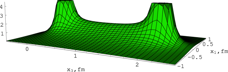
Figure 2: A distribution of the field $|\mbox{\boldmath${\rm{\cal E}}$}(x_{1},0,x_{3})|$ (32) at quark-antiquark separation 2 fm. Cutted peaks of color-Coulomb field and string between quark and antiquark are clearly distinguished. The standard values of parameters $\sigma=0.18$ GeV², $\lambda=0.2$ fm are used.

The distribution of the field $|\mbox{\boldmath${\rm{\cal E}}$}(x_{1},0,x_{3})|$ (32) is shown in Fig. 2 at $Q\bar{Q}$-separation 2 fm. One can see at the figure the peaks of the color-Coulomb field (34) over the quark and antiquark, and the string (37) between them, with the universal profile ${\cal E}(\rho)$,

$${\cal E}(\rho)=2\sigma\left(1+\frac{\rho}{\lambda}\right)\exp\left(-\frac{\rho}{\lambda}\right),$$ (39)

where $\rho$ is the distance to the $Q\bar{Q}$ axis.

3.4 Magnetic currents distribution and Londons equation

To perform more detailed analysis of the magnetic currents distribution (26) in the case of static quark and antiquark let us apply the first Maxwell equation (27) to the electric field in bilocal approximation (32), (34), (37). Then one can seethat the magnetic current ${\rm k}$ has a form

$$\mbox{\boldmath${\rm k}$}=\mathrm{rot}\,\mbox{\boldmath${\rm{\cal E}}$},$$ (40)

while the magnetic charge is absent. It is clear that the perturbative color-Coulomb field (19) does not contribute to (40). A nonperturbative field (37) is directed along the quark-antiquark axis, therefore magnetic current winds around the axis. In particular case of the saturated string (39) the polar component of the magnetic current $k_{\varphi}$ takes a form

$$k_{\varphi}(\rho)=-\frac{2\sigma\rho}{\lambda^{2}}\exp\left(-\frac{\rho}{\lambda}\right).$$ (41)

One can see that the value of the current rises linearly near the axis and falls exponentially at large distances from it.

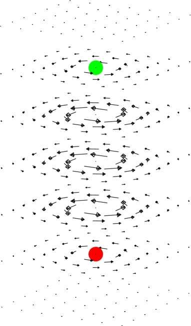
Figure 3: A vector distribution of magnetic currents (37), (40) at quark-antiquark separation 2 fm. Positions of quark and antiquark are shown by points.

The vector distribution of magnetic currents in the case of $Q\bar{Q}$-separation $R=2$ fm is shown in Fig. 3. This distribution resembles the one of the electric superconducting currents around the Abrikosov string in superconductors [91], and is another hint in favor of dual superconductivity mechanism of confinement [89]. An exponential behavior of current and field at large distances means that the dual Londons equation

$$\mathrm{rot}~{}\mbox{\boldmath${\rm k}$}=\lambda^{-2}\mbox{\boldmath${\rm{\cal E}}$}$$ (42)

is satisfied. Indeed, the only component of the polar vector $k_{\varphi}$ (41) is directed along z axes and has a form

$$(\mathrm{rot}~{}\mbox{\boldmath${\rm k}$})_{z}(\rho)=\frac{1}{\rho}\frac{\partial\rho k_{\varphi}}{\partial\rho}=\gamma(\rho)\,\lambda^{-2}{\cal E}(\rho),$$ (43)

where the universal profile ${\cal E}(\rho)$ is defined in (39), and function

$$\gamma(\rho)=\frac{-2+\rho/\lambda}{1+\rho/\lambda}$$ (44)

rises monotonically from $-2$ and at $\rho\gg\lambda$ tends to unity as $\gamma(\rho)\approx 1-3\lambda/\rho$.

One concludes that the confinement mechanism is related to cyclic magnetic currents (41) squeezing the electric field into the tube of string with the exponential fall off outside it, and satisfying the dual Londons equation (43), (44).

3.5 Vacuum polarization and screening of the coupling constant

We turn now to the second Maxwell equation for the static quark and antiquark, the Gauss law

$$\mathrm{div}\,\mbox{\boldmath${\rm{\cal E}}$}=\rho,$$ (45)

where the field ${\rm{\cal E}}$ (32) is the sum

$$\mbox{\boldmath${\rm{\cal E}}$}=\mbox{\boldmath${\rm{\cal E}}$}^{D_{1},\mathrm{oge}}+\mbox{\boldmath${\rm{\cal E}}$}^{D_{1},\mathrm{np}}+\mbox{\boldmath${\rm{\cal E}}$}^{D},$$ (46)

and $\mbox{\boldmath${\rm{\cal E}}$}^{D_{1},\mathrm{oge}}$, $\mbox{\boldmath${\rm{\cal E}}$}^{D}$ are defined in (33), (34),(37), while the nonperturbative field $\mbox{\boldmath${\rm{\cal E}}$}^{D_{1},\mathrm{np}}$ ensures the exponential fall-off of the formfactor $D_{1}$ at large distances. In this section we introduce additional assumption about charge distribution. This assumption is confirmed a posteriori by the lattice results in abelian projected gauge theory (compare e.g. the distributions of effective field and its nonperturbative part along $Q\bar{Q}$ axis in Figs. 6,7 with corresponding distributions in Fig. 21 from paper [92]). We assume that the nonperturbative contributions to the charge density cancel,

$$\mathrm{div}\,\mbox{\boldmath${\rm{\cal E}}$}^{D_{1},\mathrm{np}}=-\mathrm{div}\,\mbox{\boldmath${\rm{\cal E}}$}^{D},$$ (47)

so that the charge density has a form

$$\rho=4\pi C_{F}\alpha_{s}\,(\delta(\mbox{\boldmath${\rm r}$})-\delta(\mbox{\boldmath${\rm r}$}-\mbox{\boldmath${\rm R}$})).$$ (48)

Using explicit expression for the field $\mbox{\boldmath${\rm{\cal E}}$}^{D}$ (37), we find from (47) the “screening” charge density $\tilde{\rho}(r)$,

$$\mathrm{div}\,\mbox{\boldmath${\rm{\cal E}}$}^{D_{1},\mathrm{np}}=\tilde{\rho}(r)-\tilde{\rho}(|\mbox{\boldmath${\rm r}$}-\mbox{\boldmath${\rm R}$}|),$$ (49)

$$\tilde{\rho}(r)=-\frac{2\sigma}{\pi\lambda^{2}}\,r\,K_{1}\left(\frac{r}{\lambda}\right).$$ (50)

Relying on (49), (50), one calculates the field $\mbox{\boldmath${\rm{\cal E}}$}^{D_{1},\mathrm{np}}$,

$$\mbox{\boldmath${\rm{\cal E}}$}^{D_{1},\mathrm{np}}=\frac{\tilde{Q}(r)\,\mbox{\boldmath${\rm r}$}}{r^{3}}-\frac{{\tilde{Q}}(|\mbox{\boldmath${\rm r}$}-\mbox{\boldmath${\rm R}$}|)\,(\mbox{\boldmath${\rm r}$}-\mbox{\boldmath${\rm R}$})}{|\mbox{\boldmath${\rm r}$}-\mbox{\boldmath${\rm R}$}|^{3}},$$ (51)

where $\tilde{Q}$ is the “screening” charge,

$$\tilde{Q}(r)=\frac{2\sigma\lambda^{2}}{\pi}\int_{0}^{r/\lambda}x^{3}\,K_{1}(x)dx,$$ (52)

It is obvious that there is no field at large distances from quark and antiquark due to confinement, and the full charge $Q(r)$ defined as

$$Q(r)=C_{F}\alpha_{s}(r)-\tilde{Q}(r),$$ (53)

turns to zero. The condition $\left.Q(r)\right|_{r\to\infty}=0$ leads to the relation [40]

$$C_{F}\alpha_{s}=3\sigma\lambda^{2}$$ (54)

between the strong coupling at large distances and parameters $\sigma,\lambda$ responsible for confinement. The behavior of the charge $Q(r)$ at standard values $\sigma=0.18$ GeV², $\lambda=0.2$ fm and constant value $\alpha_{s}=0.42$ calculated from (54) is shown in Fig. 4. The mean radius of the screening according to the figure is of the order of 0.5 fm.

The behavior of the strong coupling taking into account the background confining fields was studied in [98, 99] in the framework of the background perturbation theory. It was shown that the confining background leads to the modification of the logarithmic running of coupling according to $\alpha_{s}(q^{2})\to\alpha_{s}(q^{2}+m_{B}^{2})$, where the ”background mass” $m_{B}\approx 1$ GeV$\approx\lambda^{-1}$ is related to the energy of the valence gluon excitation and the gluon correlation length. One can see that at large distances $r\gg\lambda$ the background coupling tends to constant (”freezes”), while at small ones it turns to the running coupling of the ordinary perturbation theory. The relation between parameters now takes the form

$$C_{F}\alpha_{s}(\lambda)=3\sigma\lambda^{2},$$ (55)

where $\alpha_{s}(\lambda)$ is the freezing value of background coupling equal to the ordinary running coupling at scale $\lambda$. This equation relates two alternative scale parameters of quantum theory, $\Lambda_{\mathrm{QCD}}$ and the string tension $\sigma$.

In Fig. 5 the background running coupling is shown by dotted curve. The behavior of the running charge $Q^{\mathrm{run}}(r)$ is shown by solid curve. As one can see from the figure, the effective charge has a maximum at $r\approx 0.3$ fm.

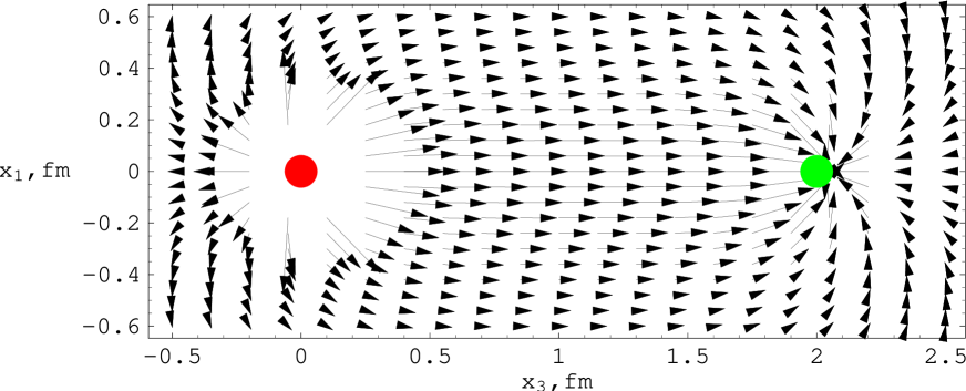
Figure 8: Vector distribution of the field $\mbox{\boldmath${\rm{\cal E}}$}(x_{1},0,x_{3})$. Positions of quark and antiquark are marked by points.

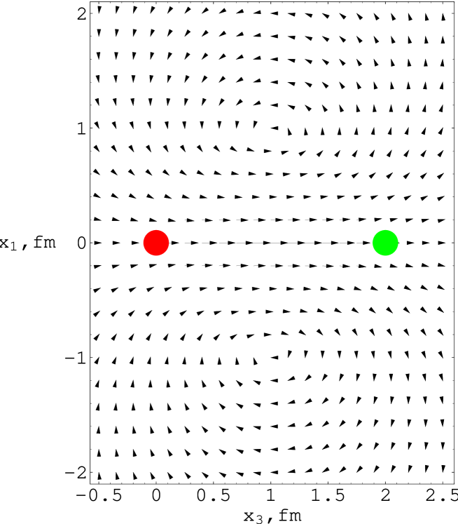
Figure 9: Vector distribution of the solenoid field $\mbox{\boldmath${\rm{\cal E}}$}^{D}(x_{1},0,x_{3})+\mbox{\boldmath${\rm{\cal E}}$}^{D_{1},\mathrm{np}}(x_{1},0,x_{3})$. Positions of quark and antiquark are marked by points.

Using standard values $\sigma=0.18$ GeV², $\lambda=0.2$ fm and constant value $\alpha_{s}=0.42$ we plot the following field distributions. In Fig. 6 the projections of fields $\mbox{\boldmath${\rm{\cal E}}$}^{D}(0,0,x_{3})$, $\mbox{\boldmath${\rm{\cal E}}$}(0,0,x_{3})$ and $\mbox{\boldmath${\rm{\cal E}}$}^{D_{1},\mathrm{oge}}(0,0,x_{3})$ into the quark-antiquark axis are shown. Note that the fields $\mbox{\boldmath${\rm{\cal E}}$}^{D_{1},\mathrm{np}}$ and $\mbox{\boldmath${\rm{\cal E}}$}^{D_{1},\mathrm{oge}}$ cancel in the middle of the string. In Fig. 7 the projections of fields $\mbox{\boldmath${\rm{\cal E}}$}^{D}(0,0,x_{3})$, $\mbox{\boldmath${\rm{\cal E}}$}^{D}(0,0,x_{3})+\mbox{\boldmath${\rm{\cal E}}$}^{D_{1},\mathrm{np}}(0,0,x_{3})$ and $\mbox{\boldmath${\rm{\cal E}}$}(0,0,x_{3})$ onto the quark-antiquark axis are plotted. In Fig. 8 the vector distribution of the displacement field $\mbox{\boldmath${\rm{\cal E}}$}(x_{1},0,x_{3})$ is shown demonstrating that the field is squeezed in tube with the width of the order of $\lambda$. In Fig. 9 the vector distribution of the solenoid field $\mbox{\boldmath${\rm{\cal E}}$}^{D}(x_{1},0,x_{3})+\mbox{\boldmath${\rm{\cal E}}$}^{D_{1},\mathrm{np}}(x_{1},0,x_{3})$ is plotted.

It is convenient to define the isotropic dielectric function $\varepsilon(r)$,

$$\varepsilon(r)=\frac{Q(r)}{C_{F}\alpha_{s}(r)}.$$ (56)

One can calculate that at large distances $r\gg\lambda$ it is exponentially small,

$$\left.\varepsilon(r)\right|_{r\to\infty}=\frac{\sqrt{\pi}}{2}\left(\frac{r}{\lambda}\right)^{5/2}\exp\left(-\frac{r}{\lambda}\right),$$ (57)

indicating the disappearence of the color-Coulomb field both inside and outside the string.

4 Hadrons with three static sources

4.1 Green functions and W-loops

Physical hadrons are nonlocal extended objects, therefore to construct their Green functions one should use nonlocal quark and gluon operators

$$q^{i}(x,Y)\equiv q^{j}(x)\Phi^{i}_{j}(x,Y),$$ (58)

$$g_{a}(x,Y)\equiv g_{b}(x)\Phi_{ab}(x,Y),$$ (59)

as well as the local one $G^{j}_{i}(x)\equiv g_{a}(x)t^{(a)j}_{i}$. Here and in what follows $i,j,...=1,2,3$ are color indexes in fundamental representation, and $a,b,...=1,..,8$ in adjoint one; $g_{a}$ denotes the valence gluon operator of background perturbation theory [98, 99], and $G^{j}_{i}(x)$ transforms as $G_{i}^{j}\to U^{+j}_{{}j^{\prime}}G_{i^{\prime}}^{j^{\prime}}U^{i^{\prime}}_{i}$ under gauge transformations. One can construct gauge invariant combinations of these operators using symmetric tensors $\delta_{i}^{j},~{}\delta^{ab},~{}d^{abc}$ and antisymmetric ones $e_{ijk}$, $f^{abc}$,

$$B_{Y}(x,y,z,Y)=e_{ijk}q^{i}(x,Y)q^{j}(y,Y)q^{k}(z,Y),$$ (60)

$$G^{(f)}_{Y}(x,y,z,Y)=f^{abc}g_{a}(x,Y)g_{b}(y,Y)g_{c}(z,Y),$$ (61)

$$G^{(d)}_{Y}(x,y,z,Y)=d^{abc}g_{a}(x,Y)g_{b}(y,Y)g_{c}(z,Y),$$ (62)

$$G_{\Delta}(x,y,z)=G_{i}^{j}(x)\Phi_{j}^{k}(x,y)G_{k}^{l}(y)\Phi_{l}^{m}(y,z)G_{m}^{n}(z)\Phi_{n}^{i}(z,x).$$ (63)

First three constructions have a structure of $Y$-type with the string junction at point $Y$, where the color indexes are contracted with the (anti-) symmetric tensor, and the latter one has a structure of triangular type. Let us stress that the wave function of triangular type is possible only for glueballs but not for baryons, see [97].

Hadron Green function has a form

$${\cal G}_{i}(\bar{X},X)=\langle\Psi^{+}_{i}(\bar{X})\Psi_{i}(X)\rangle,$$ (64)

where $\Psi_{i}=G_{\Delta},G_{Y},B_{Y};~{}X=x,y,z$ in the case of $G_{\Delta}$ and $x,y,z,Y$ for $Y$-states. The vacuum average $\langle...\rangle$ leads to the product of Green functions of quarks or valence gluons, which are proportional to the parallel transporters,

$$\langle\bar{q}_{j}(\bar{x})q^{i}(x)\rangle\sim\Phi_{j}^{i}(\bar{x},x),$$

$$\langle g_{a}(\bar{x})g_{b}(x)\rangle\sim\Phi_{ab}(\bar{x},x).$$ (65)

Therefore the hadron Green function is proportional to the W-loop of this hadron, see equation (11), and is reduced to the W-loop in the case of static sources. W-loops of baryon and $Y$-type glueball take forms correspondingly

$${\cal W}_{B}=\frac{1}{6}\langle\epsilon_{ijk}\epsilon^{i^{\prime}j^{\prime}k^{\prime}}\Phi^{i}_{i^{\prime}}(C_{1})\Phi^{j}_{j^{\prime}}(C_{2})\Phi^{k}_{k^{\prime}}(C_{3})\rangle,$$ (66)

$${\cal W}_{G}^{Y,f}=\frac{1}{24}\langle f^{abc}f^{a^{\prime}b^{\prime}c^{\prime}}\Phi^{aa^{\prime}}(C_{1})\Phi^{bb^{\prime}}(C_{2})\Phi^{cc^{\prime}}(C_{3})\rangle,$$ (67)

$${\cal W}_{G}^{Y,d}=\frac{3}{40}\langle d^{abc}d^{a^{\prime}b^{\prime}c^{\prime}}\Phi^{aa^{\prime}}(C_{1})\Phi^{bb^{\prime}}(C_{2})\Phi^{cc^{\prime}}(C_{3})\rangle.$$ (68)

Trajectories $C_{i}$ formed by the sources are shown in Fig. 10. A W-loop of $\Delta$-type glueball at large distances can be represented as a product of three meson W-loops [97],

$${\cal W}_{G}^{\Delta}(X,\bar{X})=W(\bar{x},\bar{y}|x,y)W(\bar{y},\bar{z}|y,z)W(\bar{z},\bar{x}|z,x).$$ (69)

Corresponding contours are shown in Fig. 11.

4.2 Static potentials

Static potentials of hadrons with three static sources are calculated in bilocal approximation of the field correlator method [97, 103] in the same way as meson ones. For hadrons of $Y$-type let us denote $\mbox{\boldmath${\rm n}$}^{(a)}$ the unit vector directed from the string junction to the $a$-th quark and $R_{a}$ the separation between this quark and the string junction. The potential in baryon reads

$$V_{B}(R_{1},R_{2},R_{3})=\left(\sum_{a=b}-\sum_{a<b}\right)n_{i}^{(a)}n_{j}^{(b)}\int_{0}^{R_{a}}\int_{0}^{R_{b}}dl\,dl^{\prime}\int_{0}^{\infty}dt\,{\cal D}_{i4,j4}(z_{ab}),$$ (70)

where $z_{ab}=(l\,\mbox{\boldmath${\rm n}$}^{(a)}-l^{\prime}\mbox{\boldmath${\rm n}$}^{(b)},t)$. One can represent this potential in the form

$$V_{B}=V^{c}+V^{d}+V^{\mathrm{nd}},$$ (71)

where $V^{c}$ is the color-Coulomb potential

$$V^{c}=-\frac{C_{F}\alpha_{s}}{2}\sum_{i<j}\frac{1}{r_{ij}},$$ (72)

$r_{ij}$ is the $i$-th and $j$-th quark separation. We will take into account the charge screening replacing in (72) $C_{F}\alpha_{s}$ with $Q$ defined in (53), (52). Terms $V^{d}$ and $V^{\mathrm{nd}}$ denote the diagonal and nondiagonal parts of the potential corresponding to the correlator $D$; $V^{d}$ is determined by the first and $V^{\mathrm{nd}}$ by the second sum in (70). One can find explicit expressions for $V^{d}$ and $V^{\mathrm{nd}}$ in [103]. We just note here that $V^{d}$ is a sum of quark-antiquark potentials $V^{D}$ (9), (13),

$$V^{d}(R_{1},R_{2},R_{3})=\sum_{a}V^{D}(R_{a}).$$ (73)

Characteristic feature of the potential (70) is an increase of its slope when the source separations are increasing. In Fig. 12 the behavior of the baryon potential with the color-Coulomb part subtracted is shown in comparison with the lattice data [104] as a function of the total length of baryon string $L=\sum_{a}R_{a}$. A tangent with the slope $\sigma$ is shown by points. One can see from the figure that the potential slope becomes significantly less than $\sigma$ at $L\mathrel{\mathchoice{\lower 3.6pt\vbox{\halign{$\mathsurround=0pt\displaystyle\hfil#\hfil$\cr<\crcr\sim\crcr}}}{\lower 3.6pt\vbox{\halign{$\mathsurround=0pt\textstyle\hfil#\hfil$\cr<\crcr\sim\crcr}}}{\lower 3.6pt\vbox{\halign{$\mathsurround=0pt\scriptstyle\hfil#\hfil$\cr<\crcr\sim\crcr}}}{\lower 3.6pt\vbox{\halign{$\mathsurround=0pt\scriptscriptstyle\hfil#\hfil$\cr<\crcr\sim\crcr}}}}1$ fm. This effect is induced by the influence of the correlation length of confining fields [103]. In Fig. 13 a dependence of the baryon potential in equilateral triangle on the quark separation is given in comparison with the lattice data [105]. Note the agreement between analytic and lattice calculations within the accuracy of a few tens MeV. For the $Y$-glueball potential the Casimir scaling holds,

$$\frac{V_{G}^{Y}}{V_{B}}=\frac{C_{8}}{C_{3}},$$ (74)

where $C_{3}=(N_{c}^{2}-1)/2N_{c}\equiv C_{F}$ and $C_{8}=N_{c}$ are quadratic Casimir operators in fundamental and adjoint representations.

A potential in $\Delta$-glueball in the case of equilateral triangle with the side $r$ has a form [97]

$$V_{G}^{\Delta}(r)=\frac{C_{8}}{C_{3}}V^{c}(r)+V^{d}(r)-2V^{\mathrm{nd}}(r).$$ (75)

Let us note that $V^{d}$ and $V^{\mathrm{nd}}$ depend on the valence gluons separation but not on the separation between the gluon and the center of the triangle, and that the term $-2V^{\mathrm{nd}}$ corresponds to the interaction of three effective quark-antiquark W-loops. The behavior of the potentials $V_{G}^{Y}$ and $V_{G}^{\Delta}$ in equilateral triangle in dependence on the source separation $r$ is shown in Fig. 14. The potential $V_{G}^{Y}$ goes above the $V_{G}^{\Delta}$ because of the positive contribution of nondiagonal term $V^{\mathrm{nd}}$ to $Y$-type glueball and negative to triangular one, as well as for the greater slope of diagonal term $V^{d}$ in the case of $Y$-glueball.

4.3 Fields distributions

The field in baryon is defined [40] as the square average

$$(\mbox{\boldmath${\rm{\cal E}}$}^{(B)})^{2}=\frac{2}{3}\,\left((\mbox{\boldmath${\rm{\cal E}}$}^{B}_{(1)})^{2}+(\mbox{\boldmath${\rm{\cal E}}$}^{B}_{(2)})^{2}+(\mbox{\boldmath${\rm{\cal E}}$}^{B}_{(3)})^{2}\right)$$ (76)

of fields $\mbox{\boldmath${\rm{\cal E}}$}^{B}_{(i)}$ calculated for the probe plaquette joint to the trajectory $C_{i}$,

$$\mbox{\boldmath${\rm{\cal E}}$}^{B}_{(1)}(\mbox{\boldmath${\rm x}$},\mbox{\boldmath${\rm R}$}^{(1)},\mbox{\boldmath${\rm R}$}^{(2)},\mbox{\boldmath${\rm R}$}^{(3)})=\mbox{\boldmath${\rm{\cal E}}$}^{M}(\mbox{\boldmath${\rm x}$},\mbox{\boldmath${\rm R}$}^{(1)})-\frac{1}{2}\,\mbox{\boldmath${\rm{\cal E}}$}^{M}(\mbox{\boldmath${\rm x}$},\mbox{\boldmath${\rm R}$}^{(2)})-\frac{1}{2}\,\mbox{\boldmath${\rm{\cal E}}$}^{M}(\mbox{\boldmath${\rm x}$},\mbox{\boldmath${\rm R}$}^{(3)}).$$ (77)

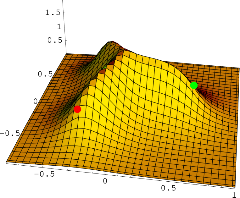
Figure 15: A distribution of the field $\mbox{\boldmath${\rm{\cal E}}$}^{(B)}$ (76), (77) in GeV/fm with the only correlator $D$ contribution considered in the quark plane for equilateral triangle with the side 1 fm. Coordinates are given in fm, positions of quarks are marked by points.

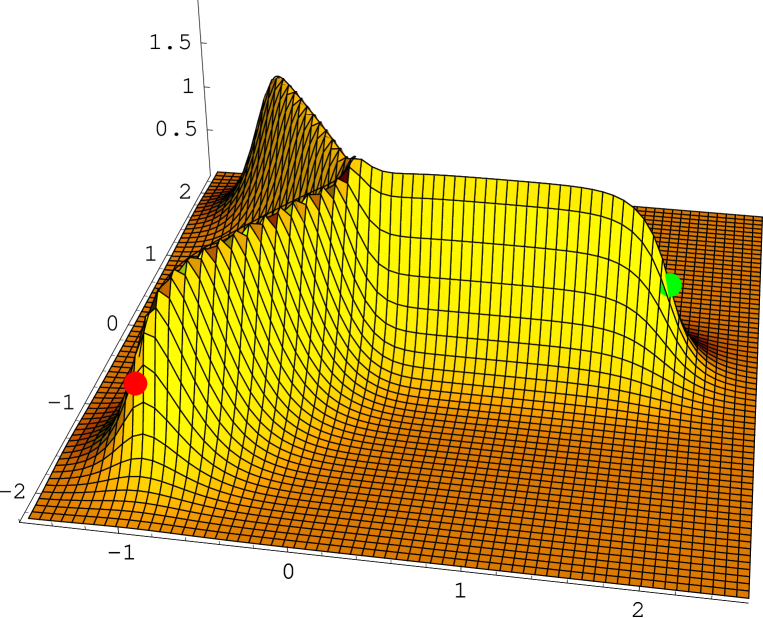
Figure 16: The same as in Fig. 15 but with the side of the equilateral triangle equal to 3.5 fm.

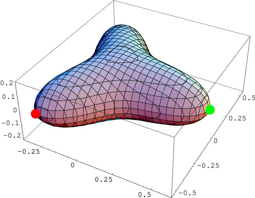
Figure 17: A surface $|\mbox{\boldmath${\rm{\cal E}}$}^{(B)}(\mbox{\boldmath${\rm x}$})|=\sigma$ at quark separations 1 fm. Coordinates are given in fm, positions of quarks are marked by points.

Normalizing coefficient 2/3 in (76) is chosen due to the condition that at large separations the field acting on quarks equals to $\sigma$. According to (76), (77), the field in baryon is expressed through fields of effective quark-antiquark pairs, with positions of antiquarks coinciding with the string junction. The distribution of the field $\mbox{\boldmath${\rm{\cal E}}$}^{(B)}$ taking into account only the contribution of formfactor $D$ is shown in Figs. 15 and 16 in the plane of quarks forming an equilateral triangle with the side 1 fm and 3.5 fm respectively. One can see in Fig. 16 three plateau with the saturated profile, and small growth of the field around the string junction point, the relative difference of values amounts to 1/16. A surface formed by the confining field with the value $\sigma$ is shown in Fig. 17 for quark separations 1 fm. One can see the small convexity in the region of the string junction.

A field in $\Delta$-type glueball is a sum of meson fields with gluon pairs acting as the effective sources [40],

$$\mbox{\boldmath${\rm{\cal E}}$}_{\Delta}^{(G)}(\mbox{\boldmath${\rm x}$},\mbox{\boldmath${\rm r}$}^{(1)},\mbox{\boldmath${\rm r}$}^{(2)},\mbox{\boldmath${\rm r}$}^{(3)})=\sum_{i=1}^{3}\mbox{\boldmath${\rm{\cal E}}$}^{M}(\mbox{\boldmath${\rm x}$}-\mbox{\boldmath${\rm r}$}^{(i)},\mbox{\boldmath${\rm r}$}^{(i+1)\mathrm{mod3}}-\mbox{\boldmath${\rm r}$}^{(i)}),$$ (78)

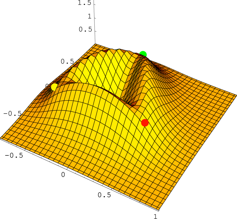
Figure 18: A distribution of the field $|\mbox{\boldmath${\rm{\cal E}}$}_{\Delta}^{(G)}(\mbox{\boldmath${\rm x}$})|$ (78) in GeV/fm of the triangular glueball in the plane of valence gluons with separations 1 fm. Coordinates are given in fm, positions of valence gluons are marked by points.

where $\mbox{\boldmath${\rm r}$}^{(i)}$ denotes the position of $i$-th valence gluon. In Fig. 18 the field distribution $|\mbox{\boldmath${\rm{\cal E}}$}_{\Delta}^{(G)}(\mbox{\boldmath${\rm x}$})|$ in valence gluon plane is shown at gluon separations 1 fm, and in Fig. 19 the surface $|\mbox{\boldmath${\rm{\cal E}}$}_{\Delta}^{(G)}(\mbox{\boldmath${\rm x}$})|=\sigma$ is plotted for the same gluon separations. Let us note that according to (38) one can calculate the static quark-antiquark potential as the work of the force acting on the quark, done on separating the latter from the antiquark to the distance $R$. Analogous relation are valid for the field and potential of $\Delta$-type glueball, see (75), (78). It is clear that the nondiagonal part of the $\Delta$-glueball potential $V^{\mathrm{nd}}$ equals to the work of force acting on the effective quark from the external string and is therefore related to the interference of the meson fields $\mbox{\boldmath${\rm{\cal E}}$}^{M}$ in the vicinity of valence gluons of the order of $\lambda$.

5 Conclusions

In this paper we have systematically treated: the vacuum fields in QCD, the confinement mechanism, the QCD string formation and finally, the field distribution inside hadrons. Everywhere we have used the field correlators as a universal gauge-invariant formalism, which allows to describe all phenomena appearing in QCD. In description of vacuum fields the most important property is the Gaussian dominance: the lowest (Gaussian) correlator is dominating on the minimal area surface of the W-loop, and there are sufficient grounds for the statement that the total distribution of higher correlators does not exceeed few percent. This phenomenon, found on the lattice [69], is not yet fully understood, see [11, 16], although it gives an explicit dynamical picture, which possibly is incompatible with the old physics of the instanton gas, of $Z_{2}$-fluxes $etc.$. Therefore, one can assert that the picture of the maximally stochastic QCD vacuum is a very good approximation to the reality. One can remember that the measure of coherence is associated with the weight of the contribution of higher correlators, e.g. for the instanton gas the total contribution of higher (non-Gaussian) correlators is dominating. Moreover, the vacuum correlation length $\lambda$ (i.e. the factor in the exponent for the asymptotics of the Gaussian correlator) is relatively small, $\lambda\sim 0.2$ fm for the quenched vacuum. This value is much smaller than the typical hadron radius, $\sim 1$ fm. Theoretically, the smallness of $\lambda$ is connected to a large mass gap for glueballs and gluelumps, since $\lambda=1/M$, where $M$ is the lowest gluelump mass, $M\sim 1.4$ GeV, which is calculated both analytically and on the lattice [12, 13, 14].

Let us turn now to the confinement mechanism. From the point of view of field correlators, confinement occurs due to the appearence of a specific term in the Gaussian correlator, denoted $D(x^{2})$, which violates Bianchi identities in the abelian case and therefore is absent in case of QED. If, however, one considers the $U(1)$ theory with magnetic monopoles present in the vacuum, then the function $D(x^{2})$ is nonzero and is proportional to the monopole current correlator. The next step is to find the source of $D(x^{2})$ (i.e. the source of confinement) in the nonabelian theory. It was done in [106, 107], where the derivatives of $D(x^{2})$ were connected to the triple correlator $\langle EEB\rangle$. Thus the problem of establishing of the confinement mechanism in the formalism of field correlators reduces to the problem of calculating $D(x^{2})$ and the triple correlator and to the finding the conditions of its appearence/disappearence (e.g. in QCD – as functions of temperature or baryon density). The lattice calculations confirm the disappearence of $D(x^{2})$ at the deconfinement temperature $T_{c}$, and with it have confirmed all cofinement picture in the framework of the present method. One expects that at the next step– by computing correlators (including $D(x^{2})$) with the help of the gluelump Green’s functions in the whole $x$ region – one will make the field correlator method selfconsistent, and the problem of confinement will be solved quantitatively and in principle.

At the same time, this universal formalism of field correlators can be used to study the distribution of effective fields and currents, defined with the help of the W-loop. This representation, see chapter 3, enables one to describe, on one hand, the dual Meissner effect [18, 19], and on the other hand, it relates to the effective Lagrangian approach of Adler and Piran [25] and dielectric vacuum models, [27, 28] and subsequent papers. Indeed, the field correlator method not only admits this approximate qualitative interpretation, but also yields explicit expressions for the density of effective electric charges and effective magnetic currents. Being the gradient of the color-Coulomb potential at small distances, the effective field condenses into a tube on the characteristic hadron scale and ensures confinement. In the process the strong coupling constant is screened due to the vacuum polarization by nonabelian gluonic interactions.

Finally, let us summarize the contents of the last chapter devoted to field distributions inside hadrons with three constituents (sources). Here the field correlator method is the only quantitative analytic method, and its comparison with numerical (lattice) results is very interesting. One can note that in the method one has only two parameters – the string tension $\sigma$ and the correlation length $\lambda$, $\lambda$ being expressed through $\sigma$, and $\sigma$ is playing the role of the scale parameter related to $\Lambda_{\mathrm{QCD}}$. The baryon potential computed in this way [103] is in good agreement with lattice calculations and gives an independent confirmation that baryon strings have the structure of the $Y$-type with the string junction. Moreover, the field correlator method explains the smaller slope of the baryon potential at the typical hadron distances, known from the baryon phenomenology – the decrease of the slope is caused by the string interference effects connected to nonzero correlation length $\lambda$. The three-gluon glueballs, in contrast to baryons, can have the structure of both $Y$-type and $\Delta$-type [97]. However, the latter is preferred energetically. In the concluding part of the last chapter the field distributions in baryons and in the $\Delta$-type glueballs are given, where one can visualize the shape of the string in these hadrons.

Summarizing, one can say that the universal language of the field correlator method turns out to be extremely convenient in all cases considered. In particular, it enables one to formulate the gauge-invariant description of the QCD vacuum as some medium with properties ensuring confinement.

The authors are grateful to L.B.Okun for his support, to N.O.Agasian, M.I.Polikarpov for discussions and to A. Di Giacomo, V.G.Bornyakov and D.V.Antonov for useful remarks. This work was supported by the grant INTAS 00-110. D.K. and Yu.S. are also supported by the grant INTAS 00-00366. V.Sh. is grateful to FOM and Dutch National Scientific Fund (NOW) for a financial support.

Figure 1: A connected probe (21) for static quark and antiquark

Figure 4: An effective charge $Q(r)$ (53) in dependence of the distance from the quark for $\sigma=0.18$ GeV², $\lambda=0.2$ fm and constant value $\alpha_{s}=0.42$.

Figure 5: A running background coupling $C_{F}\alpha_{B}(r)$ [93] (dotted curve) and running effective charge $Q^{\mathrm{run}}=C_{F}\alpha_{B}(r)-\tilde{Q}(r)$ (solid curve) vs. the distancefrom the quark.

Figure 6: Distributions of the projections of the fields $\mbox{\boldmath${\rm{\cal E}}$}^{D}(0,0,x_{3})$ (solid curve), $\mbox{\boldmath${\rm{\cal E}}$}^{D_{1},\mathrm{np}}(0,0,x_{3})$ (dashed curve) and $\mbox{\boldmath${\rm{\cal E}}$}^{D_{1},\mathrm{oge}}(0,0,x_{3})$ (dotted curve) onto the quark-antiquark axis at $Q\bar{Q}$-separation 3 fm.

Figure 7: Distributions of the projections of the fields $\mbox{\boldmath${\rm{\cal E}}$}^{D}(0,0,x_{3})$ (solid curve), $\mbox{\boldmath${\rm{\cal E}}$}^{D}(0,0,x_{3})+\mbox{\boldmath${\rm{\cal E}}$}^{D_{1},\mathrm{np}}(0,0,x_{3})$ (dashed curve) and $\mbox{\boldmath${\rm{\cal E}}$}(0,0,x_{3})$ (dotted curve) into the quark-antiquark axis at $Q\bar{Q}$-separation 3 fm.

Figure 10: A W-loop of $Y$-type.

Figure 11: A W-loop of $\Delta$-type.

Figure 12: A potential in baryon (70) with the color-Coulomb part contracted (solid curve) in comparison with the lattice data [104] points in dependence on the total length of the baryon string $L$. A value of the string tension is $\sigma=0.22$ GeV². According to (55), the corresponding value of correlation length is $\lambda=0.18$ fm.

Figure 13: A dependence of the baryon potential in equilateral triangle on quark separation $r$ (solid curve) in comparison with the lattice data [105] (points). A value of the string tension is $\sigma=0.17$ GeV² ($\lambda=0.21$ fm).

Figure 14: Potentials of three-gluon-glueballs $V_{G}^{Y}$ (solid curve) and $V_{G}^{\Delta}$ (dotte curve) in equilateral triangle vs. the sources separation $r$.

Figure 19: A surface $|\mbox{\boldmath${\rm{\cal E}}$}_{\Delta}^{(G)}(\mbox{\boldmath${\rm x}$})|=\sigma$ at valence gluons separations 1 fm. Coordinates are given in fm, positions of valence gluons are marked by points.

References

- [1] Slavnov A A, Faddeev L D, Gauge fields: an introduction to quantum theory, Addison-Wesley PC, Redwood, CA, 1991
- [2] Yndurain F J The Theory of Quark and Gluon Interactions, (3rd revised and enlarged edition, Springer, NY, 1999)
- [3] Shifman M A, Vainshtein A I, Zakharov V I Nucl. Phys.B 147 385, 448 (1979)
- [4] Simonov Yu A Phys.Uspekhi, 39 313 (1996)
- [5] Dosch H G Phys.Lett.B 190 177 (1987)
- [6] Dosch H G, Simonov Yu A Phys.Lett.B 205 339 (1988)
- [7] Simonov Yu A Nucl.Phys.B 307 512 (1988)
- [8] Di Giacomo A, Dosch H G, Shevchenko V I, Simonov Yu A Phys.Rep. 372 319 (2002)
- [9] Simonov Yu A, Tjon J Ann. Phys. 228 1 (1993)
- [10] Simonov Yu A, Tjon J Ann. Phys. 300 54 (2002)
- [11] Shevchenko V I, Simonov Yu A Int.J.Mod.Phys.A 18 127 (2003)
- [12] UKQCD Collaboration, Foster M, Michael C Nucl.Phys.Proc.Suppl. 63 724 (1998)
- [13] UKQCD Collaboration, Foster M, Michael C Phys.Rev.D 59 094509 (1999)
- [14] Simonov Yu A Nucl.Phys.B 592 350 (2001)
- [15] Simonov Yu A Phys.Atom.Nucl. 61 855 (1998)
- [16] Shevchenko V I Phys.Lett.B 550 85 (2002)
- [17] Simonov Yu A, ITEP-PH-13/97, hep-ph/0211330
- [18] ’t Hooft G, High Energy Physics (ed. A.Zicici) (Bologna, Editrici Compositori, 1976)
- [19] Mandelstam S Phys.Lett.B 53 476 (1975)
- [20] Di Giacomo A, IFUP-TH/2002-15, hep-lat/0204032
- [21] Di Giacomo A Nucl.Phys.A 702 73 (2002)
- [22] Suzuki T, Koma Y, Ito S, Ilgenfritz E-M, Park T W, Polikarpov M I Yazawa T Nucl.Phys.Proc.Suppl. 106 631 (2002)
- [23] Chernodub M N, Gubarev F V, Polikarpov M I, Zakharov V I, MPI-PhT/2001-02, hep-lat/0103033
- [24] Bornyakov V G, Komarov D A, Polikarpov M I, Veselov A I, ITEP-LAT/2002-18, hep-lat/0210047
- [25] Adler S, Piran T Phys.Lett.B 113 405 (1982)
- [26] Adler S, Piran T Rev.Mod.Phys. 56 1 (1984)
- [27] Friedberg R, Lee T D Phys.Rev.D 15 1694 (1977)
- [28] Friedberg R, Lee T D Phys.Rev.D 16 1096 (1977)
- [29] Agasian N O, Voskresensky D N Phys.Lett.B 127 448 (1983)
- [30] Migdal A B, Agasian N O, Khokhlachev S B JETP Lettrs. 41 497 (1985)
- [31] Pirner H J, Schuh A, Wilets L Phys.Lett.B 174 10 (1986)
- [32] Pirner H J, Prog.Part.Nucl.Phys. 29 33 (1992)
- [33] Traxler C T, Mosel U, Biro T S, Phys.Rev.C 59 1620 (1999)
- [34] Martens G, Greiner C, Leupold S, Mosel U, contributions to QNP 2002, hep-ph/0303017
- [35] Polyakov A M Gauge fields and strings, Harwood Academic Publishers, Chur, 1987.
- [36] Del Debbio L, Di Giacomo A, Simonov Yu A Phys.Lett.B 332 111 (1994)
- [37] Di Giacomo A, Maggiore M, Olejnik S Phys.Lett.B 236 199 (1990)
- [38] Kuzmenko D S and Simonov Yu A Phys.Lett.B 494, 81 (2000).
- [39] Kuzmenko D S, Simonov Yu A Yad.Fiz. 64 110 (2001)
- [40] Kuzmenko D S, Simonov Yu A, hep-ph/0302071, Yad.Fiz. 67, No.3 (2004) (in press)
- [41] H. Ichie, V. Bornyakov, T. Streuer, G. Schierholz, ITEP-LAT-2002-24, KANAZAWA-02-33, hep-lat/0212024.
- [42] V.Bornyakov et al. Usp.Fiz.Nauk, in press.
- [43] Bali G Phys.Rept. 343 1 (2001)
- [44] ’t Hooft G Nucl.Phys.B 72 461 (1974)
- [45] Wegner F J.Math.Phys. 12 2259 (1971)
- [46] Wilson K Phys.Rev.D 10 2445 (1974)
- [47] Volterra V, Hostinsky B, Opèrations infinitèsimale linèaires, (Gauthiers Villars, Paris, 1939)
- [48] Halpern M B Phys.Rev.D 19 517 (1979)
- [49] Bralic N Phys.Rev.D 22 3090 (1980)
- [50] Aref’eva Y Theor.Math.Phys. 43 353 (1980)
- [51] Simonov Yu A Phys.Atom.Nucl. 50 213 (1989)
- [52] Hirayama M, Ueno M Prog.Theor.Phys. 103 151 (2000)
- [53] van Kampen N G Phys.Rep. 24C 171 (1976)
- [54] van Kampen N G Physika 74 239 (1974)
- [55] Simonov Yu A, lectures at XVII international school of physics ”QCD: Perturbative or Nonperturbative?”, Lisbon, 1999, hep-ph/9911237
- [56] Eidemueller M, Jamin M Phys.Lett.B 416 415 (1998)
- [57] Shevchenko V I, ITEP-PH-01-98, hep-ph/9802274
- [58] Shevchenko V I, Simonov Yu A, Phys.Lett.B 437 131 (1998)
- [59] Mandelstam S, Phys.Rev. 175 1580 (1968)
- [60] Simonov Yu A Phys.Lett.B 464 265 (1999)
- [61] Antonov D V, Simonov Yu A it Yad.Fiz. 60 553 (1997)
- [62] Campostrini M, Di Giacomo A, Mussardo G Z.Phys.C 25 173 (1984)
- [63] Campostrini M, Di Giacomo A, Olejnik S Z.Phys.C 34 577 (1986)
- [64] Campostrini M, Di Giacomo A, Maggiore M, Panagopoulos H, Vicari E Phys.Lett.B 225 403 (1989)
- [65] Di Giacomo A, Panagopoulos H Phys.Lett.B 285 133 (1992)
- [66] Di Giacomo A, Meggiolaro E, Panagopoulos H Nucl.Phys.B 483 371 (1997)
- [67] Bali G S, Brambilla N, Vairo A Phys.Lett.B 421 265 (1998)
- [68] Simonov Yu A, Shevchenko V I Phys.Rev.D 65 074029 (2002)
- [69] Bali G Nucl.Phys.Proc.Suppl. 83 422 (2000)
- [70] Bali G Phys.Rev.D 62 114503 (2000)
- [71] Deldar S Phys.Rev.D 62 034509 (2000)
- [72] Deldar S Nucl.Phys.Proc.Suppl. 73 587 (1999)
- [73] Del Debbio L, Panagopoulos H, Rossi P, Vicari E Phys.Rev.D 65 021501 (2002)
- [74] Del Debbio L, Panagopoulos H, Rossi P, Vicari E JHEP 0201 009 (2002)
- [75] Lucini B, Teper M Phys.Lett.B 501 128 (2001)
- [76] Lucini B, Teper M Phys.Rev.D 64 105019 (2001)
- [77] L. Del Debbio, M. Faber, J. Greensite, S. Olejnik, Phys.Rev.D 53 5891 (1996)
- [78] Ambjørn J, Olesen P, Peterson C Nucl.Phys.B 240 189, 533 (1984)
- [79] Simonov Yu A JETP Lett. 71 127 (2000)
- [80] Shevchenko V I, Simonov Yu A Phys.Rev.Lett. 85 1811 (2000)
- [81] Trottier H D Phys.Lett.B 357 193 (1995)
- [82] Lee K-M Phys.Rev.D 48 2493 (1993)
- [83] Antonov D V Surveys High Energ.Phys. 14 265 (2000)
- [84] Antonov D V JHEP 0007 (2000) 055
- [85] Nachtmann O, in the proc. St.Barbara Nucl.Chrom. 183 (1985)
- [86] Kuzmenko D S hep-ph/0310017
- [87] Kuzmenko D S hep-ph/0310035, talk at Hadron’03, Aschaffenburg, Germany
- [88] Yu.A.Simonov, Lectures at the XVII International School of Physics, Lisbon, 1999, hep-ph/9911237
- [89] Nielsen H B, Olesen P Nucl.Phys.B 61 45 (1973)
- [90] Shevchenko V I, Preprint ITEP-PH-1-98, hep-ph/9802274
- [91] Abrikosov A A JETP 5 1174 (1957)
- [92] Bornyakov V G et al., hep-lat/0310011
- [93] Badalian A M, Kuzmenko D S Phys.Rev.D 65 016004 (2002)
- [94] Badalian A M, Kuzmenko D S, hep-ph/0302072, Yad.Fiz. 67, No.3 (2004) (in press)
- [95] S. Capitani et al., Nucl.Phys. B 544 (1999)
- [96] Kuzmenko D S, Simonov Yu A hep-ph/0310034, talk at Hadron’03, Aschaffenburg, Germany
- [97] Kuzmenko D S, Simonov Yu A Yad.Fiz. 66 5 (2003), hep-ph/0202277
- [98] Simonov Yu A, in Lecture Notes in Physics 479 139, (Springer-Verlag, Berlin-Heidelberg, 1996)
- [99] Simonov Yu A Phys.At.Nucl. 58 107 (1995)
- [100] Feynman R P, Phys.Rev. 80 440 (1950); ibid. 84 108 (1951)
- [101] Fock V A, Izv. AN SSSR, OMEN 557 (1937)
- [102] Schwinger J, Phys.Rev. 82 664 (1951)
- [103] Kuzmenko D S, hep-ph/0204250, Yad.Fiz. 66, No.12 (2003) (in press)
- [104] Takahashi T T et al., Phys.Rev.D 65 114509 (2002)
- [105] Alexandrou C, de Forcrand Ph, Jahn O, hep-lat/0209062
- [106] Simonov Yu A Yad.Fiz. 50 213 (1989)
- [107] Shevchenko V I, Simonov Yu A Phys. Atom. Nucl. 60 1201 (1997)