Abstract

High-precision analyses are presented for the production of scalar sleptons, selectrons and smuons in supersymmetric theories, at future $e^{+}e^{-}$ and $e^{-}e^{-}$ linear colliders. Threshold production can be exploited for measurements of the selectron and smuon masses, an essential ingredient for the reconstruction of the fundamental supersymmetric theory at high scales. The production of selectrons in the continuum will allow us to determine the Yukawa couplings in the selectron sector, scrutinizing the identity of the Yukawa and gauge couplings, which is a basic consequence of supersymmetry. The theoretical predictions are elaborated at the one-loop level in the continuum, while at threshold non-zero width effects and Sommerfeld rescattering corrections are included. The phenomenological analyses are performed for $e^{+}e^{-}$ and $e^{-}e^{-}$ linear colliders with energy up to about 1 TeV and with high integrated luminosity up to 1 ab^-1 to cover the individual slepton channels separately with high precision.

1 Introduction

Supersymmetry [1, 2] provides us with a stable bridge [3] between the electroweak scale of $\sim 10^{2}\,\,\mathrm{GeV}$ where laboratory experiments in particle physics are performed, and the Grand Unification / Planck scale of $\sim 10^{16}$ / $10^{19}\,\,\mathrm{GeV}$ where all phenomena observed at low energies are expected to be rooted in a fundamental theory including gravity. Bridging more than fourteen orders of magnitude requires a base of high precision experiments from which the extrapolation to the Planck scale can be carried out in a solid way. Such a program has already been pursued very successfully for the three gauge couplings which appear to unify at the high scale [4]. A parallel program should be carried out in supersymmetric theories for the other fundamental parameters [5], including the parameters of soft supersymmetry breaking, which may be transferred from a hidden sector near the Planck scale by gravitational interactions to our visible world.

A solid base for these extrapolations can be built by experiments at high-energy $e^{+}e^{-}$ and $e^{-}e^{-}$ colliders [6, 7, 8, 9] which, if operated with high luminosity, will enable us to map out a comprehensive and precise picture of the supersymmetric sector at the electroweak scale. After the chargino and neutralino sectors [10, 11] have been explored earlier, we will concentrate in this analysis on the charged scalar lepton sector of the first and second generation, in which mixing phenomena are expected to be strongly suppressed. [The third generation and the neutral sector will be summarized in two later addenda while the colored sector will be analyzed in a separate report.] We have elaborated the processes

$$e^{+}e^{-}\to{\tilde{\mu}}^{+}_{i}{\tilde{\mu}}^{-}_{i}\phantom{{\tilde{e}}^{+}_{i}{\tilde{e}}^{-}_{i}} [i={\rm L},{\rm R}]$$ (1)

and

$$\begin{aligned} e^{+}e^{-}&\to{\tilde{e}}^{+}_{i}{\tilde{e}}^{-}_{j}\\ e^{-}e^{-}&\to{\tilde{e}}^{-}_{i}{\tilde{e}}^{-}_{j}\end{aligned}\phantom{{\tilde{\mu}}^{+}_{i}{\tilde{\mu}}^{-}_{i}} [i,j={\rm L},{\rm R}]$$ (2)

at the level of one-loop accuracy. At the thresholds we have calculated the production cross-sections for off-shell particles including the non-zero width effects and the Coulombic Sommerfeld rescattering corrections, while in the continuum the supersymmetric one-loop corrections have been calculated for on-shell slepton production.

The threshold production of smuons, mediated by s-channel photon and $Z$-boson exchanges, proceeds through P-waves, giving rise to the moderately steep $\beta^{3}$ behavior of the cross-sections in the velocity $\beta=(1-4m_{\tilde{\mu}}^{2}/s)^{1/2}$ of the smuons. The accuracy that can be reached in measurements of the masses $m_{\tilde{\mu}_{L,R}}$ through threshold scans, is nevertheless competitive with the accuracy achieved in the continuum by reconstructing the particles through decay products in the final states. Non-diagonal and diagonal pairs of selectrons however can be excited in S-waves in $e^{+}e^{-}$ and $e^{-}e^{-}$ collisions, mediated by t-channel neutralino exchange, and they give rise to the linear $\beta$ dependence of the cross-sections near the thresholds [13]. This steep onset of the excitation curves allows us to measure the selectron masses with unrivaled precision.

Selectron production in the continuum is strongly affected by the electron-selectron-gaugino Yukawa couplings and, as result, they can be determined very precisely by measuring the cross-sections for the production processes. In this way the identity of the Yukawa couplings ($\hat{g}$) with the gauge couplings ($g$), $\hat{g}=g$, a basic consequence of supersymmetry, can be thoroughly investigated with high precision, as explored first in Ref. [14].

The threshold analyses in this report adopt techniques outlined earlier in Ref. [15]. The one-loop calculations in the continuum are performed in the dimensional reduction scheme (DRED) for regularization and with on-shell renormalization of masses and couplings. This program must be carried out consistently for the slepton sector and the neutralino sector. In the loop corrections all sectors of the electroweak supersymmetric model contribute, which in general do not decouple for large supersymmetry breaking masses [16, 17]. A remarkable feature is the appearance of anomalous threshold singularities [18], which show up as discontinuities in the cross-section as a function of the center-of-mass energy. They are induced by specific mass patterns of the particles in the loops [19], which are generally expected to be realized in supersymmetric models but which are atypical for Standard Model calculations.

The phenomenological analyses are performed in the Minimal Supersymmetric Standard Model (MSSM), based on the parameters of the mSUGRA Snowmass Point SPS1a [20]. They include effects of initial-state beamstrahlung radiation as well as the decays of the sleptons. All contributions are taken into account that lead to the same final state. They have been elaborated at the level typical for phenomenological simulations of processes at an $e^{+}e^{-}$ linear collider in the TeV range. Besides Standard Model backgrounds the most important background channels inside SUSY are taken into account explicitly. The dominant standard backgrounds, in particular from $W^{+}W^{-}$, $ZZ$ and $Z\gamma$ production, are eliminated a priori by proper cuts adopted from previous experimental studies [21]. At the level of precision required here, it is also necessary to include sub-dominant contributions from off-shell production of gauge bosons and SUSY particles.

The final picture is quite exciting: Selectron masses can be determined at an accuracy of 50 MeV, i.e. in the per-mille range, while the masses of the less frequently produced smuons are still accessible at the per-cent level. The same level of accuracy can also be realized in measurements of the Yukawa couplings of the selectron sector, thus allowing for a high-precision comparison with the corresponding gauge couplings. In summa: A high-resolution picture of the charged slepton sector in the first and second generation can be drawn by experiments at prospective $e^{+}e^{-}$ and $e^{-}e^{-}$ linear colliders.

The report is organized as follows. In Section 2 we summarize the main features of slepton production and decay in $e^{+}e^{-}$ and $e^{-}e^{-}$ collisions at the Born level. Section 3 presents the predictions for smuon and selectron production at threshold in detail, leading us to the aforementioned accuracies expected from selectron and smuon mass measurements in threshold scans. In Section 4 slepton pair production in the continuum is described, and exploited finally for measurements of the Yukawa couplings in the selectron sector. Partial results had been presented earlier in Ref. [22], while additional technical details can be found in Ref. [23]. Spectrum and properties of supersymmetric particles in the reference point SPS1a, relevant for the present study, are summarized in the Appendix for the sake of completeness and the reader’s convenience.

2 Basics of Smuon and Selectron Production and Decay

2.1 Notation and Conventions

In this report we restrict ourselves to the Minimal Supersymmetric Standard Model (MSSM) as a well-defined framework. Since the muon and electron masses are very small, the mixing among L- and R-smuon and -selectron states, partners of the left- and right-chiral leptons, can be neglected and the mass eigen-states correspond to the L,R eigen-states.

In the other sectors of the MSSM, mixing needs to be taken into account. The MSSM requires two Higgs doublets $H_{\rm u}$ and $H_{\rm d}$, which both acquire non-zero vacuum expectation values $v_{\rm u}$ and $v_{\rm d}$. The fields mix to form the Goldstone and the physical degrees of freedom with the mixing angle

$$\tan\beta\equiv v_{\rm u}/v_{\rm d},$$ (3)

given by the ratio of the vacuum expectation values.

The charged higgsinos $\widetilde{H}_{\rm u,d}^{\pm}$ and the winos $\widetilde{W}^{\pm}$ mix to form two charginos $\tilde{\chi}^{\pm}_{i}$ $(i=1,2)$, while the neutral higgsinos $\widetilde{H}_{\rm u,d}^{0}$ and the gauginos $\widetilde{B},\widetilde{W}^{0}$ form four neutralino mass eigen-states $\tilde{\chi}^{0}_{i}$ $(i=1,2,3,4)$.

Apart from the electroweak parameters, the spectrum of the charginos and neutralinos is described by three mass parameters, the Higgs/higgsino parameter $\mu$ in the superpotential and the soft SU(2) and U(1) gaugino parameters, $M_{2}$ and $M_{1}$, respectively. For the charginos the mass term reads

$$\mathcal{L}_{\rm m_{\tilde{\chi}^{\pm}}}=-\bigl{(}\widetilde{W}^{-},\widetilde{H}_{\rm d}^{-}\bigr{)}\,X\begin{pmatrix}\widetilde{W}^{+}\\ \widetilde{H}_{\rm u}^{+}\end{pmatrix}+\mbox{h.c.}$$ (4)

where $\widetilde{W}^{\pm},\widetilde{H}_{\rm u,d}^{\pm}$ are the Weyl spinors of the charged winos and higgsinos. The mass matrix

$$X=\begin{pmatrix}M_{2}&\sqrt{2}M_{\mathrm{W}}\sin\beta\\ \sqrt{2}M_{\mathrm{W}}\cos\beta&\mu\end{pmatrix}$$ (5)

can be diagonalized by two unitary matrices $U$ and $V$ according to

$$U^{*}XV^{-1} =\begin{pmatrix}m_{\tilde{\chi}^{\pm}_{1}}&0\\ 0&m_{\tilde{\chi}^{\pm}_{2}}\end{pmatrix}, \begin{pmatrix}\chi^{-}_{1}\\ \chi^{-}_{2}\end{pmatrix} =U\begin{pmatrix}\widetilde{W}^{-}\\ \widetilde{H}_{\rm d}^{-}\end{pmatrix}, \begin{pmatrix}\chi^{+}_{1}\\ \chi^{+}_{2}\end{pmatrix} =V\begin{pmatrix}\widetilde{W}^{+}\\ \widetilde{H}_{\rm u}^{+}\end{pmatrix},$$ (6)

generating the mass eigen-states $\chi^{\pm}_{i}$. In the chiral representation, the Dirac spinors $\tilde{\chi}^{\pm}_{i}$ of the charginos are constructed from the Weyl spinors as follows,

$$\tilde{\chi}^{-}_{i}=\begin{pmatrix}\chi^{-}_{i}\\[4.30554pt] \overline{\chi^{+}_{i}}\end{pmatrix}\quad\mbox{ and }\quad\tilde{\chi}^{+}_{i}=\begin{pmatrix}\chi^{+}_{i}\\[4.30554pt] \overline{\chi^{-}_{i}}\end{pmatrix}.$$ (7)

The neutralino mass term in the current eigen-basis is given by

$$\mathcal{L}_{\rm m_{\tilde{\chi}^{0}}}=-\frac{1}{2}{\psi^{0}}^{\top}\,Y\,\psi^{0}+\mbox{h.c.},\qquad\psi^{0}=\bigl{(}\widetilde{B},\widetilde{W}^{0},\widetilde{H}_{\rm d}^{0},\widetilde{H}_{\rm u}^{0}\bigr{)}^{\!\top},$$ (8)

with the symmetric mass matrix

$$Y=\begin{pmatrix}M_{1}&0&-M_{\mathrm{Z}}\,s_{{}{\mathrm{W}}}\,c_{\beta}&M_{\mathrm{Z}}\,s_{{}{\mathrm{W}}}\,s_{\beta}\\ 0&M_{2}&M_{\mathrm{Z}}\,c_{{}{\mathrm{W}}}\,c_{\beta}&-M_{\mathrm{Z}}\,c_{{}{\mathrm{W}}}\,s_{\beta}\\ -M_{\mathrm{Z}}\,s_{{}{\mathrm{W}}}\,c_{\beta}&M_{\mathrm{Z}}\,c_{{}{\mathrm{W}}}\,c_{\beta}&0&-\mu\\ M_{\mathrm{Z}}\,s_{{}{\mathrm{W}}}\,s_{\beta}&-M_{\mathrm{Z}}\,c_{{}{\mathrm{W}}}\,s_{\beta}&-\mu&0\end{pmatrix},$$ (9)

in which the abbreviations $s_{\beta}=\sin\beta$ and $c_{\beta}=\cos\beta$ have been introduced; $s_{{}{\mathrm{W}}}$ and $c_{{}{\mathrm{W}}}$ are the sine and cosine of the electroweak mixing angle. The transition to the mass eigen-basis is performed by the unitary mixing matrix $N$,

$$N^{*}YN^{-1}=\mbox{diag}\bigl{(}m_{\tilde{\chi}^{0}_{1}}^{2},m_{\tilde{\chi}^{0}_{2}}^{2},m_{\tilde{\chi}^{0}_{3}}^{2},m_{\tilde{\chi}^{0}_{4}}^{2}\bigr{)}\qquad\mbox{ with }\qquad\chi^{0}_{i}=N_{ij}\psi^{0}_{j}.$$ (10)

The Majorana spinors $\tilde{\chi}^{0}_{i}$ of the physical neutralinos are composed of the Weyl spinors as

$$\tilde{\chi}^{0}_{i}=\begin{pmatrix}\chi^{0}_{i}\\[4.30554pt] \overline{\chi^{0}_{i}}\end{pmatrix}.$$ (11)

Explicit analytical solutions for the mixing matrices can be found in Ref. [10]

2.2 Production Mechanisms

In supersymmetric theories with R-parity conservation scalar leptons are produced in pairs. Since mixing can be neglected, the pairs are built of the current eigen-states with chiral index L or R.

Process	Exchange particles	Orbital wave	Threshold excitation
$e_{\rm L}^{+}e_{\rm R}^{-}\,/\,e_{\rm R}^{+}e_{\rm L}^{-}\to{\tilde{\mu}_{\rm R}}^{+}{\tilde{\mu}_{\rm R}}^{-}\,/\,{\tilde{\mu}_{\rm L}}^{+}{\tilde{\mu}_{\rm L}}^{-}$	$\gamma,Z\phantom{,\tilde{\chi}^{0}}$	P-wave	$\propto\beta^{3}$
$e_{\rm L}^{+}e_{\rm R}^{-}\to{\tilde{e}_{\rm R}}^{+}{\tilde{e}_{\rm R}}^{-}$	$\gamma,Z,\tilde{\chi}^{0}$	P-wave	$\propto\beta^{3}$
$e_{\rm R}^{+}e_{\rm L}^{-}\to{\tilde{e}_{\rm R}}^{+}{\tilde{e}_{\rm R}}^{-}$	$\gamma,Z\phantom{,\tilde{\chi}^{0}}$	P-wave	$\propto\beta^{3}$
$e_{\rm L}^{+}e_{\rm R}^{-}\to{\tilde{e}_{\rm L}}^{+}{\tilde{e}_{\rm L}}^{-}$	$\gamma,Z\phantom{,\tilde{\chi}^{0}}$	P-wave	$\propto\beta^{3}$
$e_{\rm R}^{+}e_{\rm L}^{-}\to{\tilde{e}_{\rm L}}^{+}{\tilde{e}_{\rm L}}^{-}$	$\gamma,Z,\tilde{\chi}^{0}$	P-wave	$\propto\beta^{3}$
$e_{\rm L}^{+}e_{\rm L}^{-}\to{\tilde{e}_{\rm R}}^{+}{\tilde{e}_{\rm L}}^{-}$	$\phantom{\gamma,Z,}\tilde{\chi}^{0}$	S-wave	$\propto\beta$
$e_{\rm R}^{+}e_{\rm R}^{-}\to{\tilde{e}_{\rm L}}^{+}{\tilde{e}_{\rm R}}^{-}$	$\phantom{\gamma,Z,}\tilde{\chi}^{0}$	S-wave	$\propto\beta$
$e_{\rm R}^{-}e_{\rm R}^{-}\to{\tilde{e}_{\rm R}}^{-}{\tilde{e}_{\rm R}}^{-}$	$\phantom{\gamma,Z,}\tilde{\chi}^{0}$	S-wave	$\propto\beta$
$e_{\rm L}^{-}e_{\rm L}^{-}\to{\tilde{e}_{\rm L}}^{-}{\tilde{e}_{\rm L}}^{-}$	$\phantom{\gamma,Z,}\tilde{\chi}^{0}$	S-wave	$\propto\beta$
$e_{\rm L}^{-}e_{\rm R}^{-}\to{\tilde{e}_{\rm L}}^{-}{\tilde{e}_{\rm R}}^{-}$	$\phantom{\gamma,Z,}\tilde{\chi}^{0}$	P-wave	$\propto\beta^{3}$

Table 1: Classification of smuon and selectron production modes in terms of the exchanged particles, the orbital angular momentum of the final state wave function and the rise of the excitation curve near threshold. Specific beam polarization states are required for the individual channels.

(a)	(b)	(c)

Figure 1: Generic leading-order diagrams for the pair production of smuons and selectrons in $e^{+}e^{-}$ or $e^{-}e^{-}$ scattering.

Scalar smuons are produced in diagonal pairs via s-channel photon and $Z$-boson exchanges in $e^{+}e^{-}$ collisions, see Tab. 1 and Fig. 1 (a).

Since the intermediate state is a vector, the helicities of electron and positron must be opposite to each other. By angular momentum conservation the scalar smuons are therefore produced in P-wave states. This gives rise to the characteristic $\beta^{3}$ behavior of the excitation curves close to threshold, with $\beta$ denoting the velocity of the smuons in the final state.

The cross-sections for the production of RR and LL smuon pairs by polarized electron/positron beams may be written as

$$\sigma[e_{\rm R}^{+}\,e_{\rm L}^{-}\to{\tilde{\mu}}_{i}^{+}\,{\tilde{\mu}}_{i}^{-}] =\frac{2\pi\alpha^{2}}{3s}\beta^{3}\left[1+g_{i}\,g_{\rm L}\frac{s}{s-M_{\mathrm{Z}}^{2}}\right]^{2},$$ (12)

$$\sigma[e_{\rm L}^{+}\,e_{\rm R}^{-}\to{\tilde{\mu}}_{i}^{+}\,{\tilde{\mu}}_{i}^{-}] =\frac{2\pi\alpha^{2}}{3s}\beta^{3}\left[1+g_{i}\,g_{\rm R}\frac{s}{s-M_{\mathrm{Z}}^{2}}\right]^{2},$$ (13)

with $i={\rm L},{\rm R}$ and the left and right-chiral Z couplings

$$g_{\rm L}=\frac{-1+2s_{{}{\mathrm{W}}}^{2}}{2s_{{}{\mathrm{W}}}c_{{}{\mathrm{W}}}},\qquad g_{\rm R}=\frac{s_{{}{\mathrm{W}}}}{c_{{}{\mathrm{W}}}}.$$ (14)

As mentioned before, the polarization combinations with equal helicity of electron and positron vanish. The electromagnetic coupling $\alpha$ may conveniently be defined at the energy scale $\sqrt{s}$, incorporating properly the running of the gauge coupling.

The angular distribution of the smuons follows the familiar $\sin^{2}\theta$ rule so that the new particles are produced preferentially perpendicular to the $e^{+}e^{-}$ beam axis.

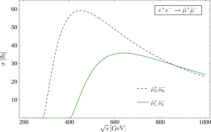
Figure 2: Born cross-sections for right- and left-chiral smuon pair production in unpolarized $e^{+}e^{-}$ annihilation.

The size of the cross-sections for smuons in the mSUGRA Snowmass point SPS1a runs up to 35 fb and 60 fb for left and right-chiral pairs, cf. Fig. 2. The cross-sections generally reach a maximum at $s\simeq 10\,m_{\tilde{\mu}}^{2}$, while for asymptotically large energies they scale as $1/s$.

Scalar electrons can be produced, besides the standard photon and $Z$-boson s-channel exchanges, via neutralino $\tilde{\chi}^{0}_{j}$ [$j=1\dots 4$] exchanges in the t-channel, cf. Tab. 1 and Fig. 1 (b,c), thereby generating, in addition to the diagonal, also non-diagonal L/R pairs. Moreover, diagonal and non-diagonal selectron pairs can be generated by t-channel neutralino exchanges in $e^{-}e^{-}$ collisions, see Fig. 1 (c).

In contrast to the vectorial s-channel amplitudes, the t-channel neutralino exchanges allow for S-wave production at the thresholds. To reduce the total angular momentum to zero, electron and positron beams are required with equal helicities. If the helicities are opposite, standard vectorial exchanges give rise to the familiar P-wave states, cf. Tab. 1.

The S-wave production processes are particularly appealing for selectron mass measurements in threshold scans due to the steep onset of the cross-sections $\propto\beta$. In $e^{+}e^{-}$ collisions only mixed selectron pairs, ${\tilde{e}_{\rm L}}{\tilde{e}_{\rm R}}$, can be produced in an S-wave, while S-wave production of diagonal selectron pairs, ${\tilde{e}_{\rm R}}{\tilde{e}_{\rm R}}$ and ${\tilde{e}_{\rm L}}{\tilde{e}_{\rm L}}$, is possible in the $e^{-}e^{-}$ mode. Moreover, $e^{-}e^{-}$ collisions provide a nearly background-free environment for selectron studies.

The Born formulae for selectron production by polarized beams read

$$\sigma[e_{-i}^{+}\,e_{i}^{-}\to{\tilde{e}}_{i}^{+}\,{\tilde{e}}_{i}^{-}] =\frac{2\pi\alpha^{2}}{3s}\beta^{3}\biggl{[}1+g_{i}^{2}\frac{s}{s-M_{\mathrm{Z}}^{2}}\biggr{]}^{2}$$

$$\;+\frac{16\pi\alpha^{2}}{s}\sum_{j=1}^{4}\sum_{k=1}^{4}|X_{ij}|^{2}\,|X_{ik}|^{2}\,h^{jk}$$ (15)

$$\;+\frac{8\pi\alpha^{2}}{s}\sum_{j=1}^{4}|X_{ij}|^{2}\left[1+g_{i}^{2}\,\frac{s}{s-M_{\mathrm{Z}}^{2}}\right]f^{j} [i={\rm L}/{\rm R},-i={\rm R}/{\rm L}],$$

$$\sigma[e_{i}^{+}\,e_{-i}^{-}\to{\tilde{e}}_{i}^{+}\,{\tilde{e}}_{i}^{-}] =\frac{2\pi\alpha^{2}}{3s}\beta^{3}\biggl{[}1+g_{i}\,g_{-i}\frac{s}{s-M_{\mathrm{Z}}^{2}}\biggr{]}^{2} [i={\rm L}/{\rm R},-i={\rm R}/{\rm L}],$$ (16)

$$\sigma[e_{\rm L}^{+}\,e_{\rm L}^{-}\to{\tilde{e}_{\rm R}}^{+}\,{\tilde{e}_{\rm L}}^{-}] =\frac{16\pi\alpha^{2}}{s}\sum_{j=1}^{4}\sum_{k=1}^{4}X_{{\rm L}j}\,X^{*}_{{\rm R}j}\,X_{{\rm R}k}\,X^{*}_{{\rm L}k}\,H^{jk},$$ (17)

$$\sigma[e_{\rm R}^{+}\,e_{\rm R}^{-}\to{\tilde{e}_{\rm L}}^{+}\,{\tilde{e}_{\rm R}}^{-}] =\sigma[e_{\rm L}^{+}\,e_{\rm L}^{-}\to{\tilde{e}_{\rm R}}^{+}\,{\tilde{e}_{\rm L}}^{-}],$$

$$\sigma[e_{i}^{-}\,e_{i}^{-}\to{\tilde{e}}_{i}^{-}\,{\tilde{e}}_{i}^{-}] =\frac{16\pi\alpha^{2}}{s}\sum_{j=1}^{4}\sum_{k=1}^{4}X_{ij}^{2}\,X^{*2}_{ik}\left[G_{+}^{jk}+H^{jk}\right] [i={\rm L}/{\rm R}],$$ (18)

$$\sigma[e_{\rm L}^{-}\,e_{\rm R}^{-}\to{\tilde{e}_{\rm L}}^{-}\,{\tilde{e}_{\rm R}}^{-}] =\frac{16\pi\alpha^{2}}{s}\sum_{j=1}^{4}\sum_{k=1}^{4}X_{{\rm L}j}^{*}\,X^{*}_{{\rm R}j}\,X_{{\rm L}k}\,X_{{\rm R}k}\,h^{jk},$$ (19)

with

$$f^{j} =\Delta_{j}\beta-\frac{\Delta_{j}^{2}-\beta^{2}}{2}\,\ln\frac{\Delta_{j}+\beta}{\Delta_{j}-\beta},$$ (20)

$$h^{jk} =\left\{\begin{array}[]{ll}\displaystyle-2\beta+\Delta_{j}\ln\frac{\Delta_{j}+\beta}{\Delta_{j}-\beta}&j=k\\ \displaystyle\frac{f^{k}-f^{j}}{\Delta_{j}-\Delta_{k}}&j\neq k\end{array}\right.,$$ (23)

$$G^{jk}_{\pm} =\frac{2}{s}\;\frac{m_{\tilde{\chi}^{0}_{j}}m_{\tilde{\chi}^{0}_{k}}}{\Delta_{j}\pm\Delta_{k}}\left[\ln\frac{\Delta_{k}+\beta}{\Delta_{k}-\beta}\pm\ln\frac{\Delta_{j}+\beta}{\Delta_{j}-\beta}\right],$$ (24)

$$H^{jk} =\left\{\begin{array}[]{ll}\displaystyle\frac{4\beta}{s}\;\frac{m_{\tilde{\chi}^{0}_{j}}^{2}}{\Delta_{j}^{2}-\beta^{2}}&j=k\\[8.61108pt] G^{ij}_{-}&j\neq k\end{array}\right.,$$ (27)

where for the case of diagonal selectron pairs, ${\tilde{e}_{\rm R}}{\tilde{e}_{\rm R}}$ and ${\tilde{e}_{\rm L}}{\tilde{e}_{\rm L}}$,

$$\Delta_{j}=\frac{2}{s}(m_{\tilde{e}_{i}}^{2}-m_{\tilde{\chi}^{0}_{j}}^{2})-1\quad{\rm and}\quad\beta=\sqrt{1-4m_{\tilde{e}_{i}}^{2}/s},$$ (28)

while for mixed pairs

$$\Delta_{j}=\frac{1}{s}(m_{\tilde{e}_{{\rm L}}}^{2}+m_{\tilde{e}_{{\rm R}}}^{2}-2m_{\tilde{\chi}^{0}_{j}}^{2})-1\quad{\rm and}\quad\beta=\frac{1}{s}\sqrt{(s-m_{\tilde{e}_{{\rm L}}}^{2}-m_{\tilde{e}_{{\rm R}}}^{2})^{2}-4m_{\tilde{e}_{{\rm L}}}^{2}m_{\tilde{e}_{{\rm R}}}^{2})^{2}}.$$ (29)

The matrix

$$X_{ij}=\bigl{[}(c_{{}{\mathrm{W}}}+g_{i}s_{{}{\mathrm{W}}})N_{j1}+(s_{{}{\mathrm{W}}}-g_{i}c_{{}{\mathrm{W}}})N_{j2}\bigr{]}/\sqrt{2}$$ (30)

accounts for the neutralino mixing with $N$ being the neutralino mixing matrix, see (10).

Since the higgsino components of the neutralino states couple with the small electron mass to the electron-selectron system, the exchange mechanism automatically projects on the gaugino components of the neutralino wave functions. The exchange of relatively light neutralinos with dominant gaugino components in the t-channel leads in general to large production cross-sections. Only if the neutralinos mass is nearly zero, the contributions associated with a Majorana mass insertion in the t-channel of amplitudes with zero total spin is suppressed. In the reference point SPS1a, however, the masses of the gaugino-like neutralinos are sufficiently large, being of the order of the slepton masses, to generate large cross-sections in all selectron channels.

(a)

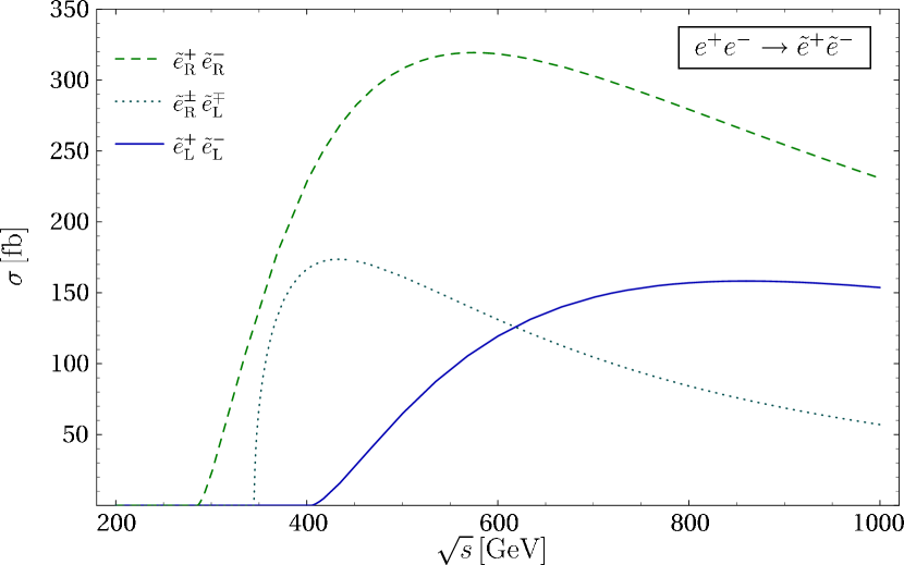
(b)

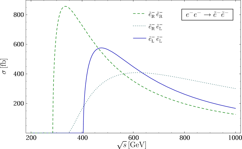
Figure 3: Born cross-sections for selectron pair production in unpolarized $e^{+}e^{-}$ (a) and
$e^{-}e^{-}$ (b) collisions.

A typical set of selectron production cross-sections is shown in Fig. 3 (a/b) for $e^{+}e^{-}$ and $e^{-}e^{-}$ collisions, respectively. As expected, the t-channel neutralino exchange enhances the cross-sections considerably. The cross-sections exceed smuon production by about an order of magnitude.

The angular sparticle distributions for the various production processes and polarized beams read

$$\frac{{\rm d}\sigma}{{\rm d}\Omega}[e_{-i}^{+}\,e_{i}^{-}\to{\tilde{e}}_{i}^{+}\,{\tilde{e}}_{i}^{-}] =\frac{\alpha^{2}}{4s}\beta^{3}\sin^{2}\theta\biggl{[}1+g_{i}^{2}\frac{s}{s-M_{\mathrm{Z}}^{2}}\biggr{]}^{2}$$

$$+\frac{4\alpha^{2}}{s}\beta^{3} \sum_{j=1}^{4}\sum_{k=1}^{4}|X_{ij}|^{2}\,|X_{ik}|^{2}\,\frac{\sin^{2}\theta}{\bigl{[}\Delta_{j}-\beta\cos\theta\bigr{]}\bigl{[}\Delta_{k}-\beta\cos\theta\bigr{]}}$$ (31)

$$+\frac{2\alpha^{2}}{s}\beta^{3} \sum_{j=1}^{4}|X_{ij}|^{2}\left[1+g_{i}^{2}\,\frac{s}{s-M_{\mathrm{Z}}^{2}}\right]\frac{\sin^{2}\theta}{\Delta_{j}-\beta\cos\theta}\qquad[i={\rm L}/{\rm R},-i={\rm R}/{\rm L}],$$

$$\frac{{\rm d}\sigma}{{\rm d}\Omega}[e_{i}^{+}\,e_{-i}^{-}\to{\tilde{e}}_{i}^{+}\,{\tilde{e}}_{i}^{-}] =\frac{\alpha^{2}}{4s}\beta^{3}\sin^{2}\theta\biggl{[}1+g_{i}\,g_{-i}\frac{s}{s-M_{\mathrm{Z}}^{2}}\biggr{]}^{2}\qquad\qquad\>[i={\rm L}/{\rm R},-i={\rm R}/{\rm L}],$$ (32)

$$\frac{{\rm d}\sigma}{{\rm d}\Omega}[e_{\rm L}^{+}\,e_{\rm L}^{-}\to{\tilde{e}_{\rm R}}^{+}\,{\tilde{e}_{\rm L}}^{-}] =\frac{16\alpha^{2}}{s}\beta\sum_{j=1}^{4}\sum_{k=1}^{4}X_{{\rm L}j}\,X^{*}_{{\rm R}j}\,X_{{\rm R}k}\,X^{*}_{{\rm L}k}\,\frac{m_{\tilde{\chi}^{0}_{j}}m_{\tilde{\chi}^{0}_{k}}/s}{\bigl{[}\Delta_{j}-\beta\cos\theta\bigr{]}\bigl{[}\Delta_{k}-\beta\cos\theta\bigr{]}},$$ (33)

$$\frac{{\rm d}\sigma}{{\rm d}\Omega}[e_{\rm R}^{+}\,e_{\rm R}^{-}\to{\tilde{e}_{\rm L}}^{+}\,{\tilde{e}_{\rm R}}^{-}] =\frac{{\rm d}\sigma}{{\rm d}\Omega}[e_{\rm L}^{+}\,e_{\rm L}^{-}\to{\tilde{e}_{\rm R}}^{+}\,{\tilde{e}_{\rm L}}^{-}],$$

$$\frac{{\rm d}\sigma}{{\rm d}\Omega}[e_{i}^{-}\,e_{i}^{-}\to{\tilde{e}}_{i}^{-}\,{\tilde{e}}_{i}^{-}] =\frac{16\alpha^{2}}{s}\beta\sum_{j=1}^{4}\sum_{k=1}^{4}X_{ij}^{2}\,X^{*2}_{ik}\frac{4\Delta_{j}\Delta_{k}\,m_{\tilde{\chi}^{0}_{j}}m_{\tilde{\chi}^{0}_{k}}/s}{\bigl{[}\Delta_{j}^{2}-\beta^{2}\cos^{2}\theta\bigr{]}\bigl{[}\Delta_{k}^{2}-\beta^{2}\cos^{2}\theta\bigr{]}}\quad\raisebox{4.30554pt}{[i = {\rm L}/{\rm R}],}$$

$$\frac{{\rm d}\sigma}{{\rm d}\Omega}[e_{\rm L}^{-}\,e_{\rm R}^{-}\to{\tilde{e}_{\rm L}}^{-}\,{\tilde{e}_{\rm R}}^{-}] =\frac{4\alpha^{2}}{s}\beta^{3}\sum_{j=1}^{4}\sum_{k=1}^{4}X_{{\rm L}j}^{*}\,X^{*}_{{\rm R}j}\,X_{{\rm L}k}\,X_{{\rm R}k}\,\frac{\sin^{2}\theta}{\bigl{[}\Delta_{j}-\beta\cos\theta\bigr{]}\bigl{[}\Delta_{k}-\beta\cos\theta\bigr{]}},$$ (35)

with $\theta$ being the angle between the incoming $e^{-}$ and the outgoing ${\tilde{e}}^{-}$ particles and $\Delta_{j}$ defined in eqs. (28), (29), respectively. Near the thresholds the angular sparticle distributions are $\propto\sin^{2}\theta$ for P-waves while S-wave distributions are isotropic. With rising center-of-mass energy, the t-channel neutralino exchange however accumulates the selectrons in the forward and backward directions as the exchange amplitudes peak near $\cos\theta\approx\pm 1$:

$$\frac{{\rm d}\sigma}{{\rm d}\cos\theta}[e^{+}\,e^{-}\to{\tilde{e}}_{i}^{+}\,{\tilde{e}}_{i}^{-}] \propto\sum_{j,k}\frac{1-\cos^{2}\theta}{\bigl{[}\Delta_{j}-\beta\cos\theta\bigr{]}\bigl{[}\Delta_{k}-\beta\cos\theta\bigr{]}}\stackrel{{\scriptstyle s\gg m_{\tilde{e}_{i}}^{2}}}{{\longrightarrow}}\frac{1+\cos\theta}{1-\cos\theta},$$ (36)

$$\frac{{\rm d}\sigma}{{\rm d}\cos\theta}[e^{+}\,e^{-}\to{\tilde{e}_{\rm R}}^{\pm}\,{\tilde{e}_{\rm L}}^{\mp}] \propto\sum_{j,k}\frac{1}{\bigl{[}\Delta_{j}-\beta\cos\theta\bigr{]}\bigl{[}\Delta_{k}-\beta\cos\theta\bigr{]}}\stackrel{{\scriptstyle s\gg m_{\tilde{e}_{i}}^{2}}}{{\longrightarrow}}\frac{1}{(1-\cos\theta)^{2}}.$$ (37)

2.3 Decay Mechanisms

The R-sleptons ${\tilde{\mu}_{\rm R}}$ and ${\tilde{e}_{\rm R}}$ are expected to decay predominantly into the lightest neutralino if the latter has a dominant bino component: ${\tilde{l}_{\rm R}}^{\pm}\to l^{\pm}\tilde{\chi}^{0}_{1}$.

The dominant decay modes of the L-sleptons ${\tilde{\mu}_{\rm L}}$ and ${\tilde{e}_{\rm L}}$ in the SPS1a scenario are also expected to be decays to the lightest neutralino. However, additional heavy neutralino cascade decays and decays to charginos generate more complicated final states [24]. The tree-level decay widths for these two-particle decays are given by

$$\Gamma[{\tilde{l}}^{-}_{i}\to l^{-}\,\tilde{\chi}^{0}_{j}] =\alpha\,|X_{ij}|^{2}\;m_{\tilde{l_{i}}}\Biggl{(}1-\frac{m_{\tilde{\chi}^{0}_{j}}^{2}}{m_{\tilde{l_{i}}}^{2}}\Biggr{)}^{\!\!2}\qquad[i={\rm L}/{\rm R},\;j=1\dots 4],$$ (38)

$$\Gamma[{\tilde{l}}^{-}_{\rm L}\to\nu_{l}\,\tilde{\chi}^{-}_{k}] =\frac{\alpha}{4}|U_{k1}|^{2}\,m_{\tilde{l_{{\rm L}}}}\Biggl{(}1-\frac{m_{\tilde{\chi}^{\pm}_{j}}^{2}}{m_{\tilde{l_{{\rm L}}}}^{2}}\Biggr{)}^{\!\!2}\qquad[k=1,2],$$ (39)

where $X$ denotes the matrix defined in eq. (30), while $U$ is the chargino mixing matrix defined in eq. (6).

Sparticle	Mass $m$ [GeV]	Decay modes
	Width $\Gamma$ [GeV]
${\tilde{l}_{\rm R}}={\tilde{e}_{\rm R}}/{\tilde{\mu}_{\rm R}}$	$m=142.72$	${\tilde{l}_{\rm R}}^{-}$	$\to l^{-}\,\tilde{\chi}^{0}_{1}$	100%
	$\Gamma=0.21$
${\tilde{l}_{\rm L}}={\tilde{e}_{\rm L}}/{\tilde{\mu}_{\rm L}}$	$m=202.32$	${\tilde{l}_{\rm L}}^{-}$	$\to l^{-}\,\tilde{\chi}^{0}_{1}$	48%
	$\Gamma=0.25$		$\to l^{-}\,\tilde{\chi}^{0}_{2}$	19%
			$\to\nu_{l}\,\tilde{\chi}^{-}_{1}$	33%
$\tilde{\chi}^{0}_{1}$	$m=96.18$	—
$\tilde{\chi}^{0}_{2}$	$m=176.62$	$\tilde{\chi}^{0}_{2}$	$\to{\tilde{e}_{\rm R}}^{\pm}\,e^{\mp}$	6%
	$\Gamma=0.020$		$\to{\tilde{\mu}_{\rm R}}^{\pm}\,\mu^{\mp}$	6%
			$\to{\tilde{\tau}_{1}}^{\pm}\,\tau^{\mp}$	88%
			$\to q\,\bar{q}\,\tilde{\chi}^{0}_{1}$	0.1%
$\tilde{\chi}_{1}^{\pm}$	$m=176.06$	$\tilde{\chi}^{+}_{1}$	$\to{\tilde{\tau}_{1}}^{+}\,\nu_{\tau}$	100%
	$\Gamma=0.014$

Table 2: Masses, widths and branching ratios of smuons, selectrons and the light neutralino and chargino states for the reference points SPS1a [20, 24].

Masses, widths and branching ratios for the reference point SPS1a [20, 24] are collected in Tab. 2. While R-sleptons decay almost exclusively into light neutralinos plus leptons, the same decay modes are also dominant for L-sleptons. Due to the fairly large value of $\tan\beta$ and, as a result, the significant stau mixing, charginos $\tilde{\chi}^{\pm}_{1}$ and the $\tilde{\chi}^{0}_{2}$ neutralinos decay primarily to $\tau$ final states, so that their experimental analysis is more demanding. As significant rates are predicted for the decay modes of the sleptons into $\tilde{\chi}^{0}_{1}$, we will focus the subsequent phenomenological analyses to these exceedingly clear channels: the final states are oppositely charged leptons plus missing energy, $e^{+}e^{-}\to l^{+}l^{-}+\makebox[2.15277pt][l]{$E$}/\,$. Decays to $\tilde{\chi}^{0}_{2}$ with subsequent $\tau$ decays can nevertheless be exploited to discriminate between L- and R-sleptons.

3 Slepton Production at Threshold and
Mass Measurements

Smuon pairs are produced in $e^{+}e^{-}$ annihilation near threshold in P-waves as a result of angular momentum conservation for spin-1 photon and $Z$-boson s-channel exchanges. This leads to the $\beta^{3}$ behavior of the excitation curve in the velocity of the produced particles. In contrast, t-channel neutralino exchanges can give rise to a steep linear beta dependence of the excitation curves for selectrons in $e^{+}e^{-}$ and $e^{-}e^{-}$ collisions, characteristic for states with zero total angular momentum.

These rules are valid at the Born level but they are modified by the non-zero widths of the produced resonances and by Sommerfeld rescattering effects generated by Coulombic photon exchange between the slowly moving final-state particles [15]. While the non-zero widths smear out the onset of the threshold excitation curves, Coulombic photon exchange enhances the cross-section near threshold. For on-shell particle production, the Coulomb correction factor is singular, $\propto\beta^{-1}$, so that the excitation curves are enhanced to $\beta^{2}$ for P-waves and they jump to non-zero values for S-waves. For the production of unstable particles, this singular behavior is alleviated by the off-shellness and finite width effects.

Moreover, studying off-shell production of sleptons, the calculation has to be performed for the final states after the decays of the resonances. Restricting ourselves to the simplest neutralino $\tilde{\chi}^{0}_{1}$ and $\tilde{\chi}^{0}_{2}$ decay modes, the processes

$$e^{+}e^{-} \to\mu^{+}\mu^{-}\,\tilde{\chi}^{0}_{1}\,\tilde{\chi}^{0}_{1}$$ (40)

and

$$e^{+}e^{-} \to e^{+}e^{-}\,\tilde{\chi}^{0}_{1,2}\,\tilde{\chi}^{0}_{1,2}$$ (41)

$$e^{-}e^{-} \to e^{-}e^{-}\,\tilde{\chi}^{0}_{1,2}\,\tilde{\chi}^{0}_{1,2}$$ (42)

must be analyzed including all channels which give rise to these final states.

The decay of L-sleptons into the next-to-lightest neutralino $\tilde{\chi}^{0}_{2}$ with the subsequent decay $\tilde{\chi}^{0}_{2}\to\tau^{+}\tau^{-}\tilde{\chi}^{0}_{1}$ (cf. Tab. 2) can be used to distinguish them from R-sleptons, which predominantly decay into the lightest neutralino $\tilde{\chi}^{0}_{1}$, i.e. ${\tilde{l}_{\rm R}}^{\pm}\to l^{\pm}\,\tilde{\chi}^{0}_{1}$. This is of particular importance since in most scenarios the R-sleptons are expected to be lighter than the corresponding L-sleptons, so that the L-sleptons are produced on top of a huge background of R-sleptons. For scenarios with $\tan\beta\,\raisebox{-1.29167pt}{${}_{\textstyle>}\atop{}^{\textstyle\sim}$}\,10$, the $\tilde{\chi}^{0}_{2}$ mainly decays into a $\tau$ pair and the lightest neutralino, so that the production of an L-slepton is signaled by the appearance of additional $\tau$ jets.

The small cross-section for L-smuon production together with the branching ratio for ${\tilde{\mu}_{\rm L}}^{\pm}\to\mu^{\pm}\,\tilde{\chi}^{0}_{2}$ results in expected event rates that are too low to perform a measurement of the threshold excitation curve. Therefore, only R-smuons, but selectrons of both L and R type will be analyzed in detail.

3.1 Off-shell Slepton Production

(a) Double resonance diagram     (b) Single resonance diagrams
       

Figure 4: The doubly and singly resonant contributions to the process $e^{+}e^{-}\to\mu^{+}\mu^{-}\tilde{\chi}^{0}_{1}\tilde{\chi}^{0}_{1}$.

The leading contribution to the $\mu^{+}\mu^{-}\,\tilde{\chi}^{0}_{1}\,\tilde{\chi}^{0}_{1}$ final state, and to electron final states correspondingly, is generated by the double resonance diagram shown in Fig. 4 (a). For invariant $\mu\tilde{\chi}^{0}_{1}$ masses near the smuon mass, the smuon propagators must be replaced by the Breit-Wigner form, which explicitly includes the non-zero width $\Gamma_{{\tilde{\mu}}}$ of the resonance state. This is achieved by substituting the complex parameter

$$m_{{\tilde{\mu}}}^{2}\;\to\;M_{{\tilde{\mu}}}^{2}=m_{{\tilde{\mu}}}^{2}-im_{{\tilde{\mu}}}\Gamma_{{\tilde{\mu}}}$$ (43)

for the smuon mass. To keep the amplitude gauge invariant, the double-resonance diagram of Fig. 4 (a) must be supplemented by the single-resonance diagrams of Fig. 4 (b).

3.2 Coulombic Sommerfeld Correction

Figure 5: Coulomb correction to smuon production, $e^{+}e^{-}\to\mu^{+}\mu^{-}\tilde{\chi}^{0}_{1}\tilde{\chi}^{0}_{1}$.

The Coulomb interaction due to photon exchange between slowly moving charged particles in Fig. 5 gives rise to large corrections to the excitation curve near threshold. For stable particles the cross-section is modified universally by the singular coefficient $\sigma_{\rm Born}\to(\alpha\pi/2\beta)\sigma_{\rm Born}$ at leading order. This Sommerfeld correction [25] removes one power of the velocity $\beta$ off the threshold suppression. For the production of off-shell particles the singularity is screened [26] and the remaining enhancement depends on the orbital angular momentum $l$. The Coulomb correction is associated with the leading term in the $\beta$ expansion of the photon exchange diagram Fig. 5. Exploiting the fact that terms with the loop momentum in the numerator generate terms proportional to $\beta$ in the diagrammatic analysis, it follows that

$$\sigma_{\rm Coul}^{\rm off-shell}=-\sigma_{\rm Born}\,\frac{\alpha s}{2\pi}\,C_{0}\;\;\Re e\!\left(\frac{2p_{+}p_{-}-2M_{\rm X}^{2}}{2p_{+}p_{-}-p_{+}^{2}-p_{-}^{2}}\right)^{l},$$ (44)

for the complex pole masses $M^{2}_{\pm}=m_{\pm}^{2}-i\,m_{\pm}\Gamma_{\!\pm}$ and the momenta $p_{\pm}$ of the slepton ${\tilde{l}}^{\pm}$, ${\tilde{l}}={\tilde{e}},{\tilde{\mu}}$. The leading part in $\beta$ of the scalar triangle function $C_{0}$ can be evaluated according to Ref. [27]. The last factor, taken to the $l$-th power, is of kinematical origin, incorporating the effect of the angular momentum $l$ of the wave function.

After carrying out the expansion for smuon and selectron P-wave production and for selectron S-wave production, the leading order can be written in the form

$$\sigma_{\rm Coul}=\sigma_{\rm Born}\,\frac{\alpha\pi}{2\beta_{p}}\biggl{[}1\!-\!\frac{2}{\pi}\arctan\frac{|{\beta_{M}}|^{2}-\beta_{p}^{2}}{2\beta_{p}\;\Im\!m\,\beta_{M}}\biggr{]}\,\Re e\biggl{[}\frac{\beta_{M}^{2}+\beta_{p}^{2}}{2\beta_{p}^{2}}\biggr{]}^{l}\qquad[l=0,1],$$ (45)

with the generalized velocities

$$\beta_{M} =\frac{1}{s}\sqrt{(s-M_{+}^{2}-M_{-}^{2})^{2}-4M_{+}^{2}M_{-}^{2}},$$ (46)

$$\beta_{p} =\frac{1}{s}\sqrt{(s-p_{+}^{2}-p_{-}^{2})^{2}-4p_{+}^{2}p_{-}^{2}}.$$ (47)

The off-shellness damps the singularities as illustrated in Fig. 6 for the S- and P-waves.

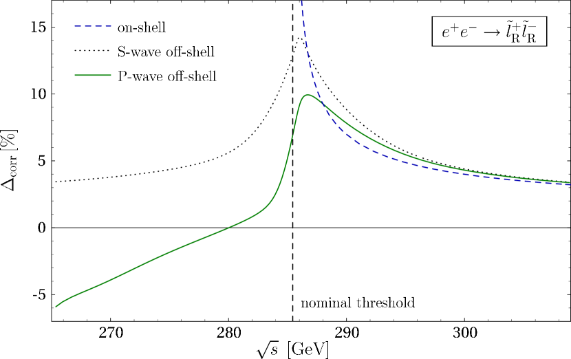
Figure 6: Correction factor $\Delta_{\rm corr}$ due to Coulomb rescattering relative to the Born cross-section for on-shell and off-shell S- and P-wave production.

3.3 Final-state Analysis

The final states in the general processes $e^{+}e^{-}\to l^{+}l^{-}+\makebox[2.15277pt][l]{$E$}/\,$ and $e^{+}e^{-}\to l^{+}l^{-}\,\tau^{+}\tau^{-}+\makebox[2.15277pt][l]{$E$}/\,$ can be generated by a large variety of background processes in addition to the signal slepton channels. Within the SUSY sector itself, pair production of charginos and neutralinos with subsequent (cascade) decays feed the final state $l^{+}l^{-}+\makebox[2.15277pt][l]{$E$}/\,$. $ZZ$ and $Zh_{0}$/$ZH_{0}$ intermediate states with one particle decaying to lepton pairs, the other to a pair of $\tilde{\chi}^{0}_{1}$ will also contribute to this class of final states. The final state with an additional tau pair is characteristic for the production of a L-slepton together with a R-slepton. SUSY backgrounds to this signature arise from neutralino production or from stau ${\tilde{\tau}}$ production with the decay chain $e^{+}e^{-}\to{\tilde{\tau}}^{+}{\tilde{\tau}}^{-}\to\tau^{+}\tau^{-}\,\tilde{\chi}^{0}_{2}\,\tilde{\chi}^{0}_{1}\to\tau^{+}\tau^{-}\,e^{+}e^{-}\,\tilde{\chi}^{0}_{1}\,\tilde{\chi}^{0}_{1}$.

Moreover, pure Standard Model processes, like the production of gauge boson pairs, $W^{+}W^{-}$, $ZZ$ and $Z\gamma^{*}$, leading to the final state $l^{+}l^{-}\nu\bar{\nu}$, also have to be taken into account. They are generically large and need to be reduced by appropriate cuts [28]. The background from resonant $Z$ production can easily be reduced by cutting on the invariant mass of the lepton pair or the invisible recoil momentum around the $Z$-pole. Contributions from $WW$ pair production have a characteristic angular distribution of the final state leptons. Because of the spin correlations and the boost factor, the leptons tend to be aligned back to back and along the beam direction. Therefore this background can be reduced effectively by rejecting signatures with back-to-back leptons. The explicit values for the cuts are summarized in Tab. 3.

Condition	Variable	Accepted range
Reject leptons in forward/ backward region from Bhabha/ Møller scattering	lepton polar angle $\theta_{\rm l}$	$|\cos\theta_{\rm l}|<0.95$
Reject soft leptons/jets from radiative photon splitting and $\gamma$-$\gamma$ background	lepton/jet energy $E_{\rm l}$	$E_{\rm l}>5$ GeV
Reject missing momentum in forward/backward region from particles lost in the beam pipe	missing momentum polar angle $\theta_{\vec{p}_{\rm miss}}$	$|\cos\theta_{\vec{p}_{\rm miss}}|<0.90$
Angular separation of two leptons	angle $\phi_{\rm l^{+}l^{-}}$ between leptons	$|1-\cos\phi_{\rm l^{+}l^{-}}|>0.002$
Angular separation of two quark or tau jets	angle $\phi_{\rm jj}$ between jets	$|1-\cos\phi_{\rm jj}|>0.015$
Cut on $Z$ decaying into lepton pair	di-lepton invariant mass $m_{\rm l^{+}l^{-}}$	$|m_{\rm l^{+}l^{-}}-M_{\mathrm{Z}}|>10$ GeV
Cut on invisibly decaying $Z$	invariant recoil mass $m_{\rm recoil}$	$|m_{\rm recoil}-M_{\mathrm{Z}}|>15$ GeV
Reject back-to-back leptons from $W$ pairs	angle $\phi_{\rm l^{+}l^{-}}$ between leptons	$|\cos\phi_{\rm l^{+}l^{-}}|<0.7$

Table 3: General cuts to reduce large Standard Model backgrounds and to account for the detector geometry and resolution.

Triple gauge boson production, $W^{+}W^{-}Z$ and $W^{+}W^{-}\gamma^{*}$, contributes to the final state $e^{+}e^{-}\to l^{+}l^{-}\,\tau^{+}\tau^{-}+\makebox[2.15277pt][l]{$E$}/\,$. The total cross-section for these processes is well below 1 fb [29] and can be reduced further by applying cuts on the invariant di-lepton mass.

The dominant supersymmetric backgrounds involve decay cascades of neutralinos and charginos that, for example following the decay chain

$$e^{+}e^{-}\to\tilde{\chi}^{0}_{1} \tilde{\chi}^{0}_{j}$$ (48)

$$\;\raisebox{4.82217pt}{$\lfloor$}\!\!\!\to l^{+}\,l^{-}\,\tilde{\chi}^{0}_{1},$$

with $j>1$, generate $l^{+}l^{-}+\makebox[2.15277pt][l]{$E$}/\,$ final states. Since the lepton pair originates only from a single neutralino decay, these backgrounds give rise to increased missing energy and lower lepton-pair invariant mass compared to the signal, and they can effectively be reduced by cuts on these two variables [15]. Near threshold an alternative method for reducing the backgrounds can be applied, based on the fact that the energy of the leptons originating from a two-body decay is defined sharply in this kinematical configuration. Thus by selecting leptons with energies in a band $\Delta E\approx 10$ GeV around the nominal threshold energy $E_{l,\rm thr}=(m_{\tilde{l}}^{2}-m_{\tilde{\chi}^{0}_{j}}^{2})/(2m_{\tilde{l}})$ greatly suppresses both SM and SUSY backgrounds. This second cut choice is applied in the following examples.

The signal-to-background ratio can further be enhanced by using beam polarization. The optimal polarization choices for the different production processes are listed in Tab. 1. As evident from the table, polarization of both the electron and positron beams can help to discriminate between the slepton chiralities (see e.g. [30]). In the following 80% polarization for the electrons and 50% polarization for the positrons is assumed. Without positron polarization the signal-to-background ratio would in general be reduced by a factor of 1.5.

For a realisitic description, it is necessary to include initial-state radiation (ISR) and beamstrahlung effects. The leading logarithmic ISR contributions are included using the structure-function method [31], while effective beamstrahlung parametrizations, taken for the Tesla design for definiteness, are adopted from the program Circe [32].

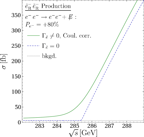
Figure 7: The excitation curves for ${\tilde{e}_{\rm R}}$ pair production over Standard Model and supersymmetric backgrounds for $e^{+}e^{-}$ annihilation (left) and $e^{-}e^{-}$ scattering (right). The signal contribution with non-zero widths and Coulomb rescattering is compared with the case of zero width and no higher order corrections. The signal is enhanced with beam polarization as indicated, where $(+)$ corresponds to right-handed and $(-)$ to left-handed polarization.

Including the SUSY and SM backgrounds, the excitation curves, after the beamstrahlung and ISR is switched on and the cuts defined before are applied, are displayed in Fig. 7 for two characteristic examples, ${\tilde{e}_{\rm R}}^{+}{\tilde{e}_{\rm R}}^{-}$ pair production in $e^{+}e^{-}$ collisions as a P-wave process, and ${\tilde{e}_{\rm R}}^{-}{\tilde{e}_{\rm R}}^{-}$ pair production in $e^{-}e^{-}$ collisions as a typical S-wave process. Separately shown are the zero-width Born prediction, the background contributions and the final prediction including non-zero width and rescattering effects, with the backgrounds added on.

Process	Fitted values for slepton mass $m$ and width $\Gamma$
$e^{+}e^{-}\to({\tilde{e}_{\rm R}}^{+}{\tilde{e}_{\rm R}}^{-})\to e^{+}e^{-}+\makebox[2.15277pt][l]{$E$}/\,$	$m_{\tilde{e}_{{\rm R}}}=142.8^{+0.21}_{-0.19}\,\,\mathrm{GeV}$	$\Gamma_{\tilde{e}_{\rm R}}=150^{+300}_{-250}\,\,\mathrm{MeV}$
$e^{-}e^{-}\to({\tilde{e}_{\rm R}}^{-}{\tilde{e}_{\rm R}}^{-})\to e^{-}e^{-}+\makebox[2.15277pt][l]{$E$}/\,$	$m_{\tilde{e}_{{\rm R}}}=142.70^{+0.048}_{-0.053}\,\,\mathrm{GeV}$	$\Gamma_{\tilde{e}_{\rm R}}=200^{+50}_{-40}\,\,\mathrm{MeV}$
$e^{+}e^{-}\to({\tilde{e}_{\rm R}}^{\pm}{\tilde{e}_{\rm L}}^{\mp})\to e^{+}e^{-}\,\tau^{+}\tau^{-}+\makebox[2.15277pt][l]{$E$}/\,$	$m_{\tilde{e}_{{\rm L}}}=202.2^{+0.37}_{-0.33}\,\,\mathrm{GeV}$	$\Gamma_{\tilde{e}_{\rm L}}=240^{+20}_{-20}\,\,\mathrm{MeV}$
$e^{-}e^{-}\to({\tilde{e}_{\rm L}}^{-}{\tilde{e}_{\rm L}}^{-})\to e^{-}e^{-}\,\tau\tau\tau\tau+\makebox[2.15277pt][l]{$E$}/\,$	$m_{\tilde{e}_{{\rm L}}}=202.1^{+0.62}_{-0.44}\,\,\mathrm{GeV}$	$\Gamma_{\tilde{e}_{\rm L}}=240^{+500}_{-240}\,\,\mathrm{MeV}$
$e^{+}e^{-}\to({\tilde{\mu}_{\rm R}}^{+}{\tilde{\mu}_{\rm R}}^{-})\to\mu^{+}\mu^{-}+\makebox[2.15277pt][l]{$E$}/\,$	$m_{\tilde{\mu}_{{\rm R}}}=142.8^{+0.42}_{-0.38}\,\,\mathrm{GeV}$	$\Gamma_{\tilde{\mu}_{\rm R}}=350^{+400}_{-400}\,\,\mathrm{MeV}$

Table 4: Expected precision for the determination of slepton masses and widths from threshold scans in $e^{+}e^{-}$ and $e^{-}e^{-}$ scattering. The reconstructed values are obtained from a four-parameter fit as outlined in the text.

The results expected from these simulations for the mass measurements are presented in Tab. 4. They are based on data simulated at five equidistant points in a center-of-mass energy range of 10 GeV in the threshold regions for ${\tilde{\mu}_{\rm R}}$ pair production, and diagonal and non-diagonal ${\tilde{e}_{\rm R}}$ and ${\tilde{e}_{\rm L}}$ production. For the $e^{+}e^{-}$ mode a total luminosity of 50 fb^-1 for each threshold scan is assumed, corresponding to 10 fb^-1 per scan point. In the $e^{-}e^{-}$ mode the anti-pinch effect leads to a somewhat reduced machine luminosity. Therefore it is presumed that a total of 5 fb^-1 is available for each scan measurement, corresponding to 1 fb^-1 per scan point. For the reconstruction of the mass a binned likelihood method is employed, using four free parameters in the fit: the slepton mass and width, a constant scale factor for the absolute normalization of the excitation curve and a constant background level. The last two parameters render the mass fit independent on details of other SUSY sectors, in particular the masses and mixings of the heavier neutralinos that are not accessible in the slepton decays.

Evidently, S-wave ${\tilde{e}_{\rm R}}$ production in $e^{-}e^{-}$ collisions provides us with mass measurements of 50 MeV, i.e. a relative error of less than 1 per-mille. This will presumably be the highest accuracy that can ever be reached for sfermion mass measurements in the supersymmetric particle sector.

4 Slepton Production in the Continuum and
Determination of Yukawa Couplings

The motivation for high-precision analyses of smuon and selectron production in the continuum is twofold, different though for the two species.

1.) Smuon pair production in the continuum serves as a rich source of particles which after subsequent decays to muons and neutralinos allows us to determine the smuon and neutralino masses. The smuon mass measurement in the continuum is competitive with the accuracy expected from threshold scans. The R-smuon decay to the lightest neutralino will be the gold-plated process (besides the analogous R-selectron decay) for measuring the mass of the lightest neutralino, which is a key particle in cosmology. Smuon pair production leads to clean $\mu^{+}\mu^{-}+\makebox[2.15277pt][l]{$E$}/\,$ final states that can easily be identified and controlled experimentally. The measurement of the cross-sections therefore provides a valuable instrument for testing supersymmetry dynamics at the quantum level.

2.) Since the precision of threshold scans in mass measurements of selectrons cannot be rivaled, the central target of selectron pair production in the continuum, besides the neutralino mass measurement [33, 21], is the analysis of the selectron-electron-neutralino Yukawa couplings in the SU(2) and U(1) sectors [16]. They are predicted to be equal to the corresponding gauge couplings in supersymmetric theories, even if the supersymmetry breaking is included by soft terms in the Lagrangian, leaving the system theoretically self-consistent. The relevant mechanism involves the t-channel exchange of neutralinos. Knowledge of the neutralino masses and mixing parameters is therefore required before high-sensitivity tests can be carried out. Thus this method is one of the components in a complex experimental program including, in addition to the analysis of selectron pair production, also pair production of charginos and neutralinos that in turn are (partly) mediated by neutral and charged slepton t-channel exchanges. The synopsis of all these channels will finally provide us with a comprehensive and detailed picture of the entire Yukawa sector in a model-independent form.

We will separate in this report the description of the theoretical techniques necessary for controlling the higher-order corrections, from the application to smuon and selectron pair production and their phenomenological evaluation, with emphasis on the analysis of Yukawa couplings.

4.1 Renormalization of the MSSM

At the one-loop level, which we work out in this report for slepton production, dimensional reduction (DRED) provides us with a valid regularization scheme including chiral currents. By reducing the kinematics in the propagation of particles to $D<4$ dimensions but leaving the number of field components unchanged, supersymmetry is preserved in the higher-order amplitudes, and so is gauge invariance [34].

Multiplicative renormalization of masses, couplings and fields can therefore be performed without introducing additional ad-hoc counter terms to restore the supersymmetry. The renormalization factors $Z$, and equivalently the shifts of variables, that absorb all the ultra-violet divergences, will be fixed by on-shell renormalization, i.e. the on-shell definition of the physical particle masses, the on-shell definition of the electromagnetic gauge couplings in the trilinear lepton-lepton-photon vertex, and normalization of the on-shell renormalized fields to unity. As a consequence of supersymmetry and gauge symmetry, the renormalization of all other quantities, Yukawa couplings, quartic couplings etc., induces calculable additional shifts. This program can be carried out consistently in theories including soft supersymmetry breaking terms.

$\parbox[c]{56.9055pt}{\psfig{width=56.9055pt}}=\parbox[c]{56.9055pt}{\psfig{width=56.9055pt}}+\parbox[c]{56.9055pt}{\psfig{width=56.9055pt}}+\parbox[c]{56.9055pt}{\psfig{width=56.9055pt}}+\parbox[c]{56.9055pt}{\psfig{width=56.9055pt}}+\parbox[c]{56.9055pt}{\psfig{width=56.9055pt}}+\parbox[c]{56.9055pt}{\psfig{width=56.9055pt}}$
$\rule{0.0pt}{0.0pt}\hskip 56.9055pt\,+\parbox[c]{56.9055pt}{\psfig{width=56.9055pt}}+\parbox[c]{56.9055pt}{\psfig{width=56.9055pt}}+\parbox[c]{56.9055pt}{\psfig{width=56.9055pt}}\phantom{+\hskip 56.9055pt+\hskip 56.9055pt+\hskip 56.9055pt\rule{0.0pt}{0.0pt}}$
$\parbox[c]{56.9055pt}{\psfig{width=54.06006pt}}=\parbox[c]{56.9055pt}{\psfig{width=54.06006pt}}+\parbox[c]{56.9055pt}{\psfig{width=54.06006pt}}\phantom{+\hskip 54.06006pt+\hskip 56.9055pt+\hskip 56.9055pt+\hskip 56.9055pt\rule{0.0pt}{0.0pt}}$
$\parbox[c]{56.9055pt}{\psfig{width=54.06006pt}}=\parbox[c]{56.9055pt}{\psfig{width=54.06006pt}}+\parbox[c]{56.9055pt}{\psfig{width=54.06006pt}}+\parbox[c]{56.9055pt}{\psfig{width=54.06006pt}}+\parbox[c]{56.9055pt}{\psfig{width=54.06006pt}}+\parbox[c]{56.9055pt}{\psfig{width=54.06006pt}}+\parbox[c]{56.9055pt}{\psfig{width=54.06006pt}}$
$\parbox[c]{56.9055pt}{\psfig{width=56.9055pt}}=\parbox[c]{56.9055pt}{\psfig{width=56.9055pt}}+\parbox[c]{56.9055pt}{\psfig{width=56.9055pt}}+\parbox[c]{56.9055pt}{\psfig{width=56.9055pt}}+\parbox[c]{56.9055pt}{\psfig{width=56.9055pt}}\phantom{+\hskip 56.9055pt+\hskip 56.9055pt\,\rule{0.0pt}{0.0pt}}$
$\parbox[c]{56.9055pt}{\psfig{width=56.9055pt}}=\parbox[c]{56.9055pt}{\psfig{width=56.9055pt}}+\parbox[c]{56.9055pt}{\psfig{width=56.9055pt}}+\parbox[c]{56.9055pt}{\psfig{width=56.9055pt}}+\parbox[c]{56.9055pt}{\psfig{width=56.9055pt}}+\parbox[c]{56.9055pt}{\psfig{width=56.9055pt}}+\parbox[c]{56.9055pt}{\psfig{width=56.9055pt}}$
$\rule{0.0pt}{0.0pt}\hskip 56.9055pt\,+\parbox[c]{56.9055pt}{\psfig{width=56.9055pt}}+\parbox[c]{56.9055pt}{\psfig{width=56.9055pt}}+\parbox[c]{56.9055pt}{\psfig{width=56.9055pt}}+\parbox[c]{56.9055pt}{\psfig{width=56.9055pt}}+\parbox[c]{56.9055pt}{\psfig{width=56.9055pt}}\phantom{+\hskip 56.9055pt\,\rule{0.0pt}{0.0pt}}$
$\parbox[c]{56.9055pt}{\psfig{width=56.9055pt}}=\parbox[c]{56.9055pt}{\psfig{width=56.9055pt}}+\parbox[c]{56.9055pt}{\psfig{width=56.9055pt}}+\parbox[c]{56.9055pt}{\psfig{width=56.9055pt}}+\parbox[c]{56.9055pt}{\psfig{width=56.9055pt}}+\parbox[c]{56.9055pt}{\psfig{width=56.9055pt}}\phantom{+\hskip 56.9055pt\,\rule{0.0pt}{0.0pt}}$

Figure 8: Generic sets of Feynman diagrams for the virtual self-energy and vertex corrections to slepton production. Solid, dashed and wiggly lines indicate fermions, (Higgs) scalars and vector bosons, respectively, whereas sfermions and gauginos are denoted by double lines and wiggly/solid lines. The selectron-electron-neutralino vertex in the last line only contributes to selectron production.

(a)                        
(b)                    

Figure 9: Box-type Feynman diagrams for slepton pair production. The first row (a) applies both to smuon and selectron production, while the second row (b) only contributes to selectron production.

Characteristic classes of higher-order diagrams for propagators and vertices are depicted in Fig. 8. Additional box diagrams, cf. Fig. 9, finally conclude the set of elements contributing to the 2-2 transitions.

(a)                                                                                      (b)
                        

Figure 10: Feynman diagrams for real photon emission in smuon production (a) and selectron production (a)+(b).

After carrying out the renormalization program in the ultraviolet sector, infrared and collinear divergences associated with the massless photon and lepton fields can be absorbed by adding the real photon emission contributions, Fig. 10. Finite results are automatically guaranteed by proceeding to experimentally well defined cross-sections, i.e. the total cross-sections in the present analysis.

Due to large number of diagrams involved, the use of computer algebra tools for the computation is necessary. The generation of diagrams and amplitudes is performed with the package FeynArts [36]. Throughout the calculation, the CKM matrix is taken diagonal and mixing between the sfermions of the first two generations is neglected. For the third generation sfermions, the mixing between the L- and R-states is consistently taken into account. A general covariant $R_{\xi}$ gauge is used in order to facilitate an additional check of the result. Using the program FeynCalc 2.2 [37], the Lorentz and Dirac algebra is evaluated and the loop integrals are reduced to a set of fundamental scalar one-loop functions [38]. Since the explicit analytical expressions of the virtual loop contributions are generally very lengthy, they have been implemented into a computer code that calculates the one-loop-corrected cross-sections, using the package LoopTools [39] for the numerical evaluation of the basic scalar one-loop functions.

4.1.1 Gauge sector

The extension of the Standard Model to a supersymmetric theory in minimal form (MSSM) does not introduce new couplings in the gauge/gaugino sector. The gauge sector of the MSSM is therefore renormalized in parallel to the Standard Model. Just the self-energies are expanded by the contributions of the supersymmetric fields in a straightforward way. We briefly summarize the results, adopting the standard conventions of Ref. [40].

The masses of the W and Z gauge bosons are shifted by

$$M_{\mathrm{W}}^{2}\to M_{\mathrm{W}}^{2}+\delta M_{\mathrm{W}}^{2}\qquad\quad\mbox{and}\qquad\quad M_{\mathrm{Z}}^{2}\to M_{\mathrm{Z}}^{2}+\delta M_{\mathrm{Z}}^{2}.$$ (49)

Imposing the on-shell renormalization conditions defined earlier, the mass shifts can be expressed in terms of the transverse self-energies $\Sigma_{\rm T}$,

$$\delta M_{\mathrm{W}}^{2}=\Re e\,\,\Sigma_{\rm T}^{\rm WW}(M_{\mathrm{W}}^{2})\qquad\quad\mbox{and}\qquad\quad\delta M_{\mathrm{Z}}^{2}=\Re e\,\,\Sigma_{\rm T}^{\rm ZZ}(M_{\mathrm{Z}}^{2}),$$ (50)

with the self-energies for the gauge boson propagation in the Standard Model expanded by supersymmetric particle contributions:

$$\Sigma_{\rm T}^{\rm V_{1}V_{2}}(k^{2})=\Sigma_{\rm T}^{\rm V_{1}V_{2}}(k^{2})\bigr{|}_{\rm SM}+\Sigma_{\rm T}^{\rm V_{1}V_{2}}(k^{2})\bigr{|}_{\rm SUSY}\qquad[{\rm V}_{i}={\rm\gamma,Z,W}].$$ (51)

The first term includes the usual Standard Model loop contributions as in the first line of Fig. 8, while the second term accounts for the additional loops involving pairs of supersymmetric fields, gaugino and sfermion fields, as given in the second line of Fig. 8.

The SU(2) and U(1) gauge couplings $g$ and $g^{\prime}$ can be traced back to the electromagnetic coupling $e$ and the electroweak weak mixing angle $s_{{}{\mathrm{W}}}=\sin\theta_{\rm W}$. $e$ is renormalized as in standard QED apart from the removal of $\gamma$-$Z$ mixing,

$$e\to(1+\delta Z_{e})\,e\qquad\mbox{with}\qquad\delta Z_{e}=\frac{1}{2}\left.\frac{\partial\Sigma^{\gamma\gamma}_{\rm T}(k^{2})}{\partial k^{2}}\right|_{k^{2}=0}-\frac{s_{{}{\mathrm{W}}}}{c_{{}{\mathrm{W}}}}\,\frac{\Sigma^{\gamma Z}_{\rm T}(0)}{M_{\mathrm{Z}}^{2}}.$$ (52)

Again the gauge-boson self-energies decompose into Standard Model and specific supersymmetric contributions as in (51).

Introducing the electroweak mixing angle in on-shell definition through the W and Z masses as $s_{{}{\mathrm{W}}}^{2}=1-M_{\mathrm{W}}^{2}/M_{\mathrm{Z}}^{2}$, the renormalized value is formally related to the bare value by

$$s_{{}{\mathrm{W}}} \to s_{{}{\mathrm{W}}}+\delta s_{{}{\mathrm{W}}} \frac{\delta s_{{}{\mathrm{W}}}}{s_{{}{\mathrm{W}}}} =\frac{c_{{}{\mathrm{W}}}^{2}}{2s_{{}{\mathrm{W}}}^{2}}\left[\frac{\delta M_{\mathrm{Z}}^{2}}{M_{\mathrm{Z}}^{2}}-\frac{\delta M_{\mathrm{W}}^{2}}{M_{\mathrm{W}}^{2}}\right].$$ with (53)

Finally, the renormalized left- and right-handed electron fields,

$$e_{\rm L} \to(1+\tfrac{1}{2}\delta Z^{e\rm L})\,e_{\rm L}, e_{\rm R} \to(1+\tfrac{1}{2}\delta Z^{e\rm R})\,e_{\rm R},$$ (54)

are related to the electron self-energies by

$$\delta Z^{e\rm L} =-\Re e\,\biggl{\{}\Sigma^{e\rm L}(m_{\mathrm{e}}^{2})+m_{\mathrm{e}}^{2}\,\frac{\partial}{\partial p^{2}}\Bigl{[}\Sigma^{e\rm L}(p^{2})+\Sigma^{e\rm R}(p^{2})+2/m_{\mathrm{e}}\,\Sigma^{e\rm S}(p^{2})\Bigr{]}_{p^{2}=m_{\mathrm{e}}^{2}}\biggr{\}},$$ (55)

$$\delta Z^{e\rm R} =-\Re e\,\biggl{\{}\Sigma^{e\rm R}(m_{\mathrm{e}}^{2})+m_{\mathrm{e}}^{2}\,\frac{\partial}{\partial p^{2}}\Bigl{[}\Sigma^{e\rm L}(p^{2})+\Sigma^{e\rm R}(p^{2})+2/m_{\mathrm{e}}\,\Sigma^{e\rm S}(p^{2})\Bigr{]}_{p^{2}=m_{\mathrm{e}}^{2}}\biggr{\}},$$ (56)

with the decomposition

$$\Sigma^{e}(p)\,=\,\makebox[0.86108pt][l]{$p$}/\,\omega_{\rm L}\Sigma^{e\rm L}(p^{2})\;+\makebox[0.86108pt][l]{$p$}/\,\omega_{\rm R}\Sigma^{e\rm R}(p^{2})+\Sigma^{e\rm S}(p^{2})\qquad\mbox{with}\qquad\omega_{{\rm L},{\rm R}}=(1\pm\gamma_{5})/2.\\$$ (57)

Apart from the calculation of the (singular) QED corrections, the chiral limit of vanishing electron mass can be safely applied, simplifying eqs. (55), (56) to

$$\delta Z^{e\rm L}_{\rm weak} =-\Re e\,\,\Sigma^{e\rm L}_{\rm weak}(0), \delta Z^{e\rm R}_{\rm weak} =-\Re e\,\,\Sigma^{e\rm R}_{\rm weak}(0).$$ (58)

4.1.2 Sfermion sector

In the limit of vanishing lepton masses in the first and second generation, the L- and R-selectron and smuon fields do not mix and the mass matrices are approximately diagonal. The “chiral” L and R states coincide with the mass eigen-states. This remains true in higher orders as the sfermion mixing is proportional to the associated lepton mass. The L and R fields may therefore be treated independently so that the renormalization follows the standard procedure. With

$$m_{\tilde{l_{i}}}^{2}\to m_{\tilde{l_{i}}}^{2}+\delta m_{\tilde{l_{i}}}^{2}\qquad\mbox{and}\qquad{\tilde{l}}_{i}\to(1+\tfrac{1}{2}\delta Z^{\tilde{l}}_{i})\,{\tilde{l}}_{i}\qquad[l=e,\mu;i={\rm L},{\rm R}],$$ (59)

we find for the sfermion mass shift

$$\delta m_{\tilde{l_{i}}}^{2}=\Re e\,\Sigma^{\tilde{l}}_{i}(m_{\tilde{l_{i}}}^{2}),$$ (60)

and for the wave-function renormalization

$$\delta Z^{\tilde{l}}_{i}=-\Re e\,\frac{\partial\Sigma^{\tilde{l}}_{i}(k^{2})}{\partial k^{2}}\biggr{|}_{k^{2}=m_{\tilde{l_{i}}}^{2}}$$ (61)

Here $\Sigma^{\tilde{l}}_{i}(k^{2})$ denotes the self-energy for the slepton ${\tilde{l}}_{i}$; $l=e,\mu$; $i={\rm L},{\rm R}$. Since the external fields are superpartners, the slepton self-energies cannot be separated into a Standard Model and a genuinely supersymmetric part.

Note that the mass shift and wave-function renormalization for L-sneutrinos coincide with those of L-selectrons in the chiral limit we consider in this report.

4.1.3 Chargino and neutralino sector

The spectrum of two charginos and four neutralinos in the MSSM is described by the three mass parameters $\mu$, $M_{2}$ and $M_{1}$, see section 2.1. Apart from other electroweak parameters, the system is also affected by the Higgs mixing $\tan\beta$. Three chargino/neutralino masses are sufficient to fix the mass parameters $\mu$, $M_{2}$ and $M_{1}$. The renormalization of $\tan\beta$ is performed outside the chargino and neutralino sector, as will be discussed in section 4.1.4

The other three masses and the mixing parameters are then uniquely determined once the parameters in the loop corrections are known [41, 42]. Following [41], the renormalization is performed in the current eigen-basis.

1.) Starting from the chargino Lagrangian

$${\cal L}_{\rm ch}=i\bigl{[}{\psi^{-}}^{\top}\sigma^{\mu}\partial_{\mu}\,\overline{\psi^{-}}+\overline{\psi^{+}}^{\top}\bar{\sigma}^{\mu}\partial_{\mu}\,{\psi^{+}}\bigr{]}-\bigl{[}{\psi^{-}}^{\top}X\,{\psi^{+}}+\overline{\psi^{+}}^{\top}X^{\dagger}\,\overline{\psi^{-}}\,\bigr{]},$$ (62)

with the current fields

$$\psi^{+}\equiv\begin{pmatrix}\psi^{+}_{1}\\ \psi^{+}_{2}\end{pmatrix}=\begin{pmatrix}\widetilde{W}^{+}\\ \widetilde{H}_{\rm u}^{+}\end{pmatrix},\;\;\;\;\;\psi^{-}\equiv\begin{pmatrix}\psi^{-}_{1}\\ \psi^{-}_{2}\end{pmatrix}=\begin{pmatrix}\widetilde{W}^{-}\\ \widetilde{H}_{\rm d}^{-}\end{pmatrix},$$ (63)

the mass matrix $X$ is renormalized by

$$X\to X+\delta X\quad\mbox{with}\qquad\delta X=\begin{pmatrix}\delta M_{2}&\sqrt{2}\;\delta\left(M_{\mathrm{W}}\sin\beta\right)\\ \sqrt{2}\;\delta\left(M_{\mathrm{W}}\cos\beta\right)&\delta\mu\end{pmatrix},$$ (64)

and the current fields are replaced by the normalized mass eigen-fields $\chi^{\pm}$,

$$\psi^{+}\to V^{\dagger}\left(1+\tfrac{1}{2}\delta\tilde{Z}^{\mathrm{L}}\right)\chi^{+},\qquad\psi^{-}\to U^{\dagger}\left(1+\tfrac{1}{2}\delta\tilde{Z}^{\mathrm{R}}\right)\chi^{-}.$$ (65)

Besides the renormalization of the new parameters $\mu$ and $M_{2}$, $\delta X$ includes the renormalization of $\tan\beta$ and the W mass discussed earlier. The [infinite] multiplicative renormalization of the wave functions is absorbed in the matrices $\delta\tilde{Z}^{\mathrm{L}},\delta\tilde{Z}^{\mathrm{R}}$, and so is the [finite] renormalization of the matrices $V,U$ rotating the current to the mass fields. The renormalized chargino Lagrangian and the associated counter terms may be written in the form

$${\cal L}_{\rm ch} \to{\cal L}_{\rm ch}+\delta{\cal L}_{\rm ch},$$

$${\cal L}_{\rm ch} =\begin{pmatrix}\overline{\tilde{\chi}^{+}_{1}},\!\!\!&\overline{\tilde{\chi}^{+}_{2}}\end{pmatrix}\left[i\makebox[0.6458pt][l]{$\partial$}/-U^{*}XV^{\dagger}\,\omega_{\rm L}-VX^{\dagger}U^{\top}\omega_{\rm R}\right]\begin{pmatrix}\tilde{\chi}^{+}_{1}\\ \tilde{\chi}^{+}_{2}\end{pmatrix},$$ (66)

$$\delta{\cal L}_{\rm ch} =\begin{pmatrix}\overline{\tilde{\chi}^{+}_{1}},\!\!\!&\overline{\tilde{\chi}^{+}_{2}}\end{pmatrix}\biggl{[}i\frac{\makebox[0.6458pt][l]{$\partial$}/}{2}\bigl{(}{\delta\tilde{Z}^{\mathrm{L}}}^{\dagger}+\delta\tilde{Z}^{\mathrm{L}}\bigr{)}\,\omega_{\rm L}+i\frac{\makebox[0.6458pt][l]{$\partial$}/}{2}\bigl{(}{\delta\tilde{Z}^{\mathrm{R}}}^{*}+{\delta\tilde{Z}^{\mathrm{R}}}^{\top}\bigr{)}\,\omega_{\rm R}$$

$$\qquad-\bigl{(}\tfrac{1}{2}{\delta\tilde{Z}^{\mathrm{R}}}^{\top}U^{*}XV^{\dagger}+\tfrac{1}{2}U^{*}XV^{\dagger}\delta\tilde{Z}^{\mathrm{L}}+U^{*}\delta XV^{\dagger}\bigr{)}\,\omega_{\rm L}$$ (67)

$$\qquad-\bigl{(}\tfrac{1}{2}{\delta\tilde{Z}^{\mathrm{L}}}^{\dagger}VX^{\dagger}U^{\top}+\tfrac{1}{2}VX^{\dagger}U^{\top}{\delta\tilde{Z}^{\mathrm{R}}}^{*}+V\delta X^{\dagger}U^{\top}\bigr{)}\,\omega_{\rm R}\biggr{]}\begin{pmatrix}\tilde{\chi}^{+}_{1}\\ \tilde{\chi}^{+}_{2}\end{pmatrix}.$$

The physical $\chi^{\pm}$ masses can be introduced in (66) after diagonalizing this part of the Lagrangian by rotation through $U,V$. The counterterms $\delta\mu$ and $\delta M_{2}$ can thereby be adjusted such that the propagator matrix develops poles at the on-shell chargino masses $m_{\tilde{\chi}^{\pm}_{1,2}}$. In addition, the $\tilde{Z}^{{\rm L},{\rm R}}$ factors can be uniquely fixed by requiring that the propagator matrix is diagonal and that the pole residues are normalized to unity for on-shell momenta.

2.) The analogous program can be carried out in the neutralino system, though the doubling of degrees of freedom renders the analysis more cumbersome. The bilinear part of the neutralino Lagrangian in the current eigen-basis is given by

$${\cal L}_{\rm n}=\frac{i}{2}\bigl{[}{\psi^{0}}^{\top}\sigma^{\mu}\partial_{\mu}\,\overline{\psi^{0}}+\overline{\psi^{0}}^{\top}\bar{\sigma}^{\mu}\partial_{\mu}\,{\psi^{0}}\bigr{]}-\frac{1}{2}\bigl{[}{\psi^{0}}^{\top}Y\,{\psi^{0}}+\overline{\psi^{0}}^{\top}Y^{\dagger}\,\overline{\psi^{0}}\,\bigr{]},$$ (68)

with $\psi^{0}$ and $Y$ given in (8) and (9), respectively. In this representation the renormalization of the mass matrix $Y$ is defined as

$$Y \to Y+\delta Y,$$

with

$$\delta Y =\begin{pmatrix}\delta M_{1}&0&-\delta(M_{\mathrm{Z}}\,s_{{}{\mathrm{W}}}\,c_{\beta})&\delta(M_{\mathrm{Z}}\,s_{{}{\mathrm{W}}}\,s_{\beta})\\ 0&\delta M_{2}&\delta(M_{\mathrm{Z}}\,c_{{}{\mathrm{W}}}\,c_{\beta})&-\delta(M_{\mathrm{Z}}\,c_{{}{\mathrm{W}}}\,s_{\beta})\\ -\delta(M_{\mathrm{Z}}\,s_{{}{\mathrm{W}}}\,c_{\beta})&\delta(M_{\mathrm{Z}}\,c_{{}{\mathrm{W}}}\,c_{\beta})&0&-\delta\mu\\ \delta(M_{\mathrm{Z}}\,s_{{}{\mathrm{W}}}\,s_{\beta})&-\delta(M_{\mathrm{Z}}\,c_{{}{\mathrm{W}}}\,s_{\beta})&-\delta\mu&0\end{pmatrix},$$ (69)

while the renormalization and the rotation from current fields $\psi^{0}$ to mass eigen-spinors $\chi^{0}$ can be performed as

$$\psi^{0}\to N^{\dagger}\left(1+\tfrac{1}{2}\delta\tilde{Z}^{0}\right)\chi^{0}.$$ (70)

The matrix $\delta\tilde{Z}^{0}$ absorbs the multiplicative renormalization of the current fields as well as the renormalization of the rotation matrix. Thus the renormalized neutralino Lagrangian can be cast into the form

$${\cal L}_{\rm n} \to{\cal L}_{\rm n}+\delta{\cal L}_{\rm n},$$

$${\cal L}_{\rm n} =\frac{1}{2}\begin{pmatrix}\overline{\tilde{\chi}^{0}_{1}},\!\!\!&\overline{\tilde{\chi}^{0}_{2}}\end{pmatrix}\left[i\makebox[0.6458pt][l]{$\partial$}/-N^{*}YN^{\dagger}\,\omega_{\rm L}-NY^{\dagger}N^{\top}\omega_{\rm R}\right]\begin{pmatrix}\tilde{\chi}^{0}_{1}\\ \tilde{\chi}^{0}_{2}\end{pmatrix},$$ (71)

together with the counter terms

$$\delta{\cal L}_{\rm n} =\frac{1}{2}\begin{pmatrix}\overline{\tilde{\chi}^{0}_{1}},\!\!\!&\overline{\tilde{\chi}^{0}_{2}}\end{pmatrix}\biggl{[}i\frac{\makebox[0.6458pt][l]{$\partial$}/}{2}\bigl{(}{\delta\tilde{Z}^{0}}^{\dagger}+\delta\tilde{Z}^{0}\bigr{)}\,\omega_{\rm L}+i\frac{\makebox[0.6458pt][l]{$\partial$}/}{2}\bigl{(}{\delta\tilde{Z}^{0}}^{*}+{\delta\tilde{Z}^{0}}^{\top}\bigr{)}\,\omega_{\rm R}$$

$$\qquad-\bigl{(}\tfrac{1}{2}{\delta\tilde{Z}^{0}}^{\top}N^{*}YN^{\dagger}+\tfrac{1}{2}N^{*}YN^{\dagger}\delta\tilde{Z}^{0}+N^{*}\delta YN^{\dagger}\bigr{)}\,\omega_{\rm L}$$ (72)

$$\qquad-\bigl{(}\tfrac{1}{2}{\delta\tilde{Z}^{0}}^{\dagger}NY^{\dagger}N^{\top}+\tfrac{1}{2}NY^{\dagger}N^{\top}{\delta\tilde{Z}^{0}}^{*}+N\delta Y^{\dagger}N^{\top}\bigr{)}\,\omega_{\rm R}\biggr{]}\begin{pmatrix}\tilde{\chi}^{0}_{1}\\ \tilde{\chi}^{0}_{2}\end{pmatrix}.$$

where the matrix $N$ rotates the neutralino mass matrix into diagonal form according to (10). The mass $m_{\tilde{\chi}^{0}_{1}}$ of the lightest neutralino $\tilde{\chi}^{0}_{1}$, that will be under excellent experimental control, may be chosen to define the remaining U(1) gaugino mass parameter $M_{1}$. The masses of the heavier neutralinos are thereafter fixed uniquely by the Higgs/higgsino and gaugino parameters $\mu$ and $M_{2,1}$. Again, the elements of the $\tilde{Z}^{0}$ wave-function renormalization matrix can be adjusted such that the elements of the neutralino propagator matrix are diagonal with unit residues of the mass poles for on-shell momenta.

In the case of CP conservation, the renormalization of the Higgs/higgsino parameter $\mu$ and the gaugino parameters $M_{1}$ and $M_{2}$ may be cast in the following form

$$\delta M_{2} =\!\!\begin{aligned} \Bigl{[}&\tfrac{1}{2}(m_{\tilde{\chi}^{\pm}_{2}}\mu-m_{\tilde{\chi}^{\pm}_{1}}M_{2})\;\Re e\,\!\bigl{\{}m_{\tilde{\chi}^{\pm}_{1}}\Sigma^{\pm{\mathrm{L}}}_{11}(m_{\tilde{\chi}^{\pm}_{1}}^{2})+m_{\tilde{\chi}^{\pm}_{1}}\Sigma^{\pm{\mathrm{R}}}_{11}(m_{\tilde{\chi}^{\pm}_{1}}^{2})+2\,\Sigma^{\pm{\mathrm{SL}}}_{11}(m_{\tilde{\chi}^{\pm}_{1}}^{2})\bigr{\}}\\ +&\tfrac{1}{2}(m_{\tilde{\chi}^{\pm}_{1}}\mu-m_{\tilde{\chi}^{\pm}_{2}}M_{2})\;\Re e\,\!\bigl{\{}m_{\tilde{\chi}^{\pm}_{2}}\Sigma^{\pm{\mathrm{L}}}_{22}(m_{\tilde{\chi}^{\pm}_{2}}^{2})+m_{\tilde{\chi}^{\pm}_{2}}\Sigma^{\pm{\mathrm{R}}}_{22}(m_{\tilde{\chi}^{\pm}_{2}}^{2})+2\,\Sigma^{\pm{\mathrm{SL}}}_{22}(m_{\tilde{\chi}^{\pm}_{2}}^{2})\bigr{\}}\\ +&M_{2}\;\delta M_{\mathrm{W}}^{2}+\mu\;\delta\bigl{(}M_{\mathrm{W}}^{2}\sin 2\beta\bigr{)}\Bigr{]}\,/\,(\mu^{2}-M_{2}^{2}),\end{aligned}$$ (73)

$$\delta\mu =\!\!\begin{aligned} \Bigl{[}&\tfrac{1}{2}(m_{\tilde{\chi}^{\pm}_{2}}M_{2}-m_{\tilde{\chi}^{\pm}_{1}}\mu)\;\Re e\,\!\bigl{\{}m_{\tilde{\chi}^{\pm}_{1}}\Sigma^{\pm{\mathrm{L}}}_{11}(m_{\tilde{\chi}^{\pm}_{1}}^{2})+m_{\tilde{\chi}^{\pm}_{1}}\Sigma^{\pm{\mathrm{R}}}_{11}(m_{\tilde{\chi}^{\pm}_{1}}^{2})+2\,\Sigma^{\pm{\mathrm{SL}}}_{11}(m_{\tilde{\chi}^{\pm}_{1}}^{2})\bigr{\}}\\ +&\tfrac{1}{2}(m_{\tilde{\chi}^{\pm}_{1}}M_{2}-m_{\tilde{\chi}^{\pm}_{2}}\mu)\;\Re e\,\!\bigl{\{}m_{\tilde{\chi}^{\pm}_{2}}\Sigma^{\pm{\mathrm{L}}}_{22}(m_{\tilde{\chi}^{\pm}_{2}}^{2})+m_{\tilde{\chi}^{\pm}_{2}}\Sigma^{\pm{\mathrm{R}}}_{22}(m_{\tilde{\chi}^{\pm}_{2}}^{2})+2\,\Sigma^{\pm{\mathrm{SL}}}_{22}(m_{\tilde{\chi}^{\pm}_{2}}^{2})\bigr{\}}\\ +&\mu\;\delta M_{\mathrm{W}}^{2}+M_{2}\;\delta\bigl{(}M_{\mathrm{W}}^{2}\sin 2\beta\bigr{)}\Bigr{]}\,/\,(M_{2}^{2}-\mu^{2}),\end{aligned}$$ (74)

$$\delta M_{1} =\begin{aligned} \frac{1}{N_{11}^{2}}\Bigl{[}&\Re e\,\!\bigl{\{}m_{\tilde{\chi}^{0}_{1}}\Sigma^{0{\mathrm{L}}}_{11}(m_{\tilde{\chi}^{0}_{1}}^{2})+\Sigma^{0{\mathrm{SL}}}_{11}(m_{\tilde{\chi}^{0}_{1}}^{2})\bigr{\}}-N_{12}^{2}\,\delta M_{2}+2N_{13}N_{14}\,\delta\mu\\ +\;&2N_{11}\bigl{[}N_{13}\;\delta\bigl{(}M_{\mathrm{Z}}s_{{}{\mathrm{W}}}\cos\beta\bigr{)}-N_{14}\;\delta\bigl{(}M_{\mathrm{Z}}s_{{}{\mathrm{W}}}\sin\beta\bigr{)}\bigr{]}\\ +\;&2N_{12}\bigl{[}N_{13}\;\delta\bigl{(}M_{\mathrm{Z}}c_{{}{\mathrm{W}}}\cos\beta\bigr{)}-N_{14}\;\delta\bigl{(}M_{\mathrm{Z}}c_{{}{\mathrm{W}}}\sin\beta\bigr{)}\bigr{]}\Bigr{]},\end{aligned}$$ (75)

which is in agreement with [41]. Here the following decomposition of the chargino/neutralino self-energies has been used:

$$\Sigma^{\chi}_{ij}(p)=\makebox[0.86108pt][l]{$p$}/\,\omega_{\rm L}\Sigma^{\chi{\mathrm{L}}}_{ij}(p^{2})\;+\makebox[0.86108pt][l]{$p$}/\,\omega_{\rm R}\Sigma^{\chi{\mathrm{R}}}_{ij}(p^{2})+\omega_{\rm L}\Sigma^{\chi{\mathrm{SL}}}_{ij}(p^{2})+\omega_{\rm R}\Sigma^{\chi{\mathrm{SR}}}_{ij}(p^{2}).$$ (76)

The combinations of self-energies in (73)–(75) are equivalent to the counterterms of the on-shell chargino and neutralino masses,

$$\delta m_{\tilde{\chi}^{\pm}_{k}} =\frac{1}{2}\,\Re e\,\!\bigl{\{}m_{\tilde{\chi}^{\pm}_{k}}\Sigma^{\pm{\mathrm{L}}}_{kk}(m_{\tilde{\chi}^{\pm}_{k}}^{2})+m_{\tilde{\chi}^{\pm}_{k}}\Sigma^{\pm{\mathrm{R}}}_{kk}(m_{\tilde{\chi}^{\pm}_{k}}^{2})+2\,\Sigma^{\pm{\mathrm{SL}}}_{kk}(m_{\tilde{\chi}^{\pm}_{k}}^{2})\bigr{\}}\qquad[k=1,2],$$ (77)

$$\delta m_{\tilde{\chi}^{0}_{1}} =\phantom{\frac{1}{2}\,}\Re e\,\!\bigl{\{}m_{\tilde{\chi}^{0}_{1}}\Sigma^{0{\mathrm{L}}}_{11}(m_{\tilde{\chi}^{0}_{1}}^{2})+\Sigma^{0{\mathrm{SL}}}_{11}(m_{\tilde{\chi}^{0}_{1}}^{2})\bigr{\}}.$$ (78)

Once the two $\tilde{\chi}^{\pm}_{1,2}$ chargino masses and the $\tilde{\chi}^{0}_{1}$ mass are fixed, the remaining heavier neutralino masses are shifted by finite amounts relative to the Born terms [which, by definition, are the eigenvalues of the renormalized mass matrix [41, 35]],

$$m_{\tilde{\chi}^{0}_{k}}-m_{\tilde{\chi}^{0}_{k}}^{\rm Born}=-\Re e\,\!\bigl{\{}m_{\tilde{\chi}^{0}_{k}}\Sigma^{0{\mathrm{L}}}_{kk}(m_{\tilde{\chi}^{0}_{k}}^{2})+\Sigma^{0{\mathrm{SL}}}_{kk}(m_{\tilde{\chi}^{0}_{k}}^{2})\bigr{\}}+(N^{*}\delta YN^{\dagger})_{kk}\qquad[k=2,3,4].$$ (79)

The cancellation of the divergences between the neutralino self-energies and the mass matrix counterterm $\delta Y$ in this expression is a non-trivial check of the method.

4.1.4 Higgs mixing $\tan\beta$

At tree level, the Higgs mixing parameter $\tan\beta$ is determined by three soft SUSY breaking parameters, the diagonal mass parameters $m_{1}^{2}$ and $m_{2}^{2}$ as well as the $H_{\rm u}$–$H_{\rm d}$ mixing term $m_{3}^{2}$, that is connected with the soft parameter $B\mu$. They define the bilinear part of the scalar potential of the two Higgs doublets,

$$H_{\rm u}=\begin{pmatrix}\phi^{+}_{\rm u}\\ v_{\rm u}+\tfrac{1}{\sqrt{2}}(\phi_{\rm u}+i\rho_{\rm u})\end{pmatrix}\qquad\mbox{and}\qquad H_{\rm d}=\begin{pmatrix}v_{\rm d}+\tfrac{1}{\sqrt{2}}(\phi_{\rm d}+i\rho_{\rm d})\\ -\phi^{-}_{\rm d}\end{pmatrix},$$ (80)

$$\begin{gathered}V_{\rm bilin}=m_{1}^{2}\left(\tfrac{1}{2}\phi_{\rm d}^{2}+\tfrac{1}{2}\rho_{\rm d}^{2}+|\phi^{-}_{\rm d}|^{2}\right)+m_{2}^{2}\left(\tfrac{1}{2}\phi_{\rm u}^{2}+\tfrac{1}{2}\rho_{\rm u}^{2}+|\phi^{+}_{\rm u}|^{2}\right)\\ +m_{3}^{2}\left(\phi_{\rm u}\phi_{\rm d}+\rho_{\rm u}\rho_{\rm d}+\phi^{+}_{\rm u}\phi^{-}_{\rm d}+{\phi^{+}_{\rm u}}^{*}{\phi^{-}_{\rm d}}^{*}\right).\end{gathered}$$ (81)

The three soft SUSY breaking parameters can be reexpressed in terms of the vacuum expectation values $v_{\rm u}$ and $v_{\rm d}$, and the pseudoscalar mass $M_{\mathrm{A}}$. The tree-level relation $\tan\beta=v_{\rm u}/v_{\rm d}$ is modified by higher-order corrections to the Higgs potential and needs to be renormalized.

Various renormalization prescriptions have been proposed in the literature, which however do not lead to satisfactory solutions on all accounts [43]. Renormalization prescriptions that are derived from the Higgs potential introduce dangerously large corrections to $\tan\beta$, which effectively invalidate the convergence of the perturbation series. Other methods impose the renormalization condition that the Goldstone bosons to not mix with the physical Higgs bosons for on-shell momenta [44], but the value of $\tan\beta$ in these schemes depends on the gauge choice.

Alternatively, one may define $\tan\beta$ in higher orders by relating it to a specific physical process. However, any definition of $\tan\beta$ through a physical process is afflicted with technical difficulties that are introduced by the particular process. Moreover, the value of $\tan\beta$ may be extracted from different observables, for example from Higgs decays [45, 43], Higgs production processes [46], or from the cross-sections for mixed chargino pair production for moderate values of $\tan\beta\,\raisebox{-0.43057pt}{${}_{\textstyle<}\atop{}^{\textstyle\sim}$}\,10$ [10], while for large $\tan\beta$ the $\tau$ polarization in $\tilde{\tau}$ decays provides an attractive opportunity [47]. Any such approach does not lead to a unique and universal choice for the renormalization of $\tan\beta$.

In the following analysis we adopt the most convenient solution by just subtracting the divergent part in the $\overline{\rm DR}$ scheme from the unrenormalized parameter to define the renormalized parameter. Without loss of generality, the universal $\overline{\rm DR}$ counterterm for $\tan\beta$ may be extracted from the mixing self-energy of the $Z$-boson and the pseudo-scalar Higgs boson $A^{0}$, with the natural choice for the renormalization scale being the $A^{0}$-mass $M_{\mathrm{A}}$:

$$\tan\beta\to\tan\beta+\delta\tan\beta\qquad\mbox{with}\qquad\delta\tan\beta=-\frac{1}{2\cos^{2}\beta\,M_{\mathrm{Z}}}\,\Im m\,\,\Sigma_{A^{0}Z}(M_{\mathrm{A}}^{2})\big{|}_{\rm div},$$ (82)

with the subscript “div” indicating that only the divergent part of the self-energy is retained.

Though being process-independent, this definition is not perfect either as the value depends on the chosen gauge. [By accident it remains independent on the gauge fixing parameter $\xi$ in the $R_{\xi}$ gauge to one-loop order]. Of course, the predictions for physical observables remain gauge independent as the gauge dependence of $\tan\beta|_{\overline{\rm DR}}$ is neutralized by equivalent terms in the amplitudes themselves.

4.2 Effective Yukawa Couplings

In general, quantum corrections are reduced with increasing mass of the virtual particles inside the loops, as generally expected by the uncertainty principle and formalized by the decoupling theorem [48]. However, in theories with broken symmetries, these corrections may grow to large values if the mass splitting in the particle multiplets is large. High mass scales in theories with broken symmetries can thus manifest themselves in the radiative corrections to precision observables at much lower energies. A classical example for this phenomenon is provided by the mass splitting in the top-bottom iso-doublet of the Standard Model [49] which strongly affects the $\rho$ parameter in the ratio of $W$- and $Z$-boson masses.

In theories with broken supersymmetry such a phenomenon arises if the splitting between the masses of SM particles and some of the SUSY partners becomes very large [such scenarios are realized, for instance, in focus point theories [50]], leading to superoblique corrections that grow logarithmically with the mass splitting [16, 17]. The splitting affects in particular the relation between the gauge couplings and the associated Yukawa couplings. In parallel to the bare couplings, the renormalized Yukawa couplings can naturally be defined to be the same as the gauge couplings at the renormalization point if supersymmetry is broken softly. Accordingly, in the on-shell renormalization scheme the renormalized Yukawa couplings are defined to be equal to the renormalized on-shell gauge couplings, so that the renormalized Lagrangian manifestly reflects the supersymmetry [modulo the soft-breaking terms]. Nevertheless, the loops will modify in toto the two types of vertices associated with the two couplings differently in physical amplitudes evaluated near the light SUSY scale, or equivalently the electroweak scale. In a more intuitive language, the running of the two couplings with energy from the high SUSY mass scale down to the low SUSY mass scale (or electroweak scale) is different [16, 17].

(a)	(b)

Figure 11: Quark-squark loop corrections (a) to the U(1) and (b) to the SU(2) neutral gaugino self-energies.

These effects are rooted in the self-energies of the gaugino lines, shown in Fig. 11 (a) and (b) for bino and wino lines, respectively. In parallel to the iso-multiplets of the Standard Model, the non-decoupling corrections arise from large mass splittings within the supersymmetric particle spectrum, for example for exceedingly high squark masses. The wave-function renormalization associated with these diagrams can be projected onto effective U(1) and SU(2) Yukawa couplings, $\hat{g}^{\prime}_{\rm eff}$ and $\hat{g}_{\rm eff}$, defined near the light SUSY/electroweak scale $M_{\rm ew}$; in the same way as the wave-function renormalization $Z^{\gamma}$ of the photon defines the effective electromagnetic coupling $e_{\rm eff}$ = $\sqrt{Z^{\gamma}}\,e$.

The self-energy correction derived from Fig. 11 (a) for the U(1) bino propagator is given, in leading logarithmic order of the ratio between the large SUSY and the electroweak scale, by

$$\Sigma^{0}_{\rm\tilde{B},log}(p)=-\!\makebox[0.86108pt][l]{$p$}/\,\frac{g^{\prime 2}}{16\pi^{2}}\,\frac{11}{2}\,\ln M_{\tilde{\rm Q}}^{2}/M_{\rm ew}^{2}.$$ (83)

This may be reinterpreted as a shift of the effective U(1) Yukawa coupling,

$$\frac{\hat{g}^{\prime 2}_{\rm eff}}{\hat{g}^{\prime 2}_{0}}=1+\frac{g^{\prime 2}}{16\pi^{2}}\,\frac{11}{2}\,\ln M_{\tilde{\rm Q}}^{2}/M_{\rm ew}^{2}$$ (84)

in leading logarithmic approximation, in relation to the bare Yukawa/gauge couplings $\hat{g}^{\prime}_{0}=g^{\prime}_{0}$. The effective U(1) gauge coupling $g^{\prime 2}_{\rm eff,log}$ can be introduced in parallel. It is identical to the renormalized gauge coupling $g^{\prime}$ in the on-shell scheme,

$$\frac{g^{\prime 2}_{\rm eff}}{g^{\prime 2}_{0}}=1+\frac{g^{\prime 2}}{16\pi^{2}}\,\frac{11}{6}\,\ln M_{\tilde{\rm Q}}^{2}/M_{\rm ew}^{2}.$$ (85)

The ratio of U(1) Yukawa to gauge coupling is therefore given effectively by

$$\frac{\hat{g}^{\prime 2}_{\rm eff}}{g^{\prime 2}_{\rm eff}}=1+\frac{g^{\prime 2}}{16\pi^{2}}\,\frac{11}{3}\,\ln M_{\tilde{\rm Q}}^{2}/M_{\rm ew}^{2}.$$ (86)

Thus, even in spite of the fundamental identity of the renormalized Yukawa and gauge couplings in supersymmetric theories in soft SUSY breaking scenarios, we find nevertheless logarithmically enhanced departures from universality in effective couplings at the electroweak scale if the mass splitting in the supersymmetric multiplets is large.

The SU(2) Yukawa and gauge couplings can be treated analogously. From the wino self-energy in Fig. 11 (b) the effective SU(2) Yukawa coupling $\hat{g}^{2}_{\rm eff}$ can be defined. Together with the on-shell renormalization of the SU(2) gauge coupling $g$, this leads to

$$\frac{\hat{g}^{2}_{\rm eff}}{g^{2}_{\rm eff}}=1+\frac{g^{2}}{16\pi^{2}}\,3\,\ln M_{\tilde{\rm Q}}^{2}/M_{\rm ew}^{2}$$ (87)

for the ratio of the two effective Yukawa and gauge couplings in leading logarithmic order.

The logarithmic growth of the one-loop corrections will later be analyzed numerically when the production of selectron pairs, involving the Yukawa couplings in t-channel neutralino exchange amplitudes, will be compared with the production of smuon pairs in detail.

4.3 Anomalous Thresholds

Figure 12: Vertex graph for the process $e^{+}e^{-}\to{\tilde{\mu}}^{+}{\tilde{\mu}}^{-}$ that bears an anomalous threshold for the mass hierarchy $m_{\tilde{\chi}^{0}_{1}}<m_{\tilde{\mu}}<m_{\tilde{\chi}^{0}_{4}}$.

The rich pattern of different masses in supersymmetric theories gives rise to anomalous threshold singularities [18, 19] in vertex and box graphs [which play no role in general in the Standard Model]. While the vertex graph for $e^{+}e^{-}\to{\tilde{\mu}}^{+}{\tilde{\mu}}^{-}$ in Fig. 12 generates a normal threshold singularity when the energy $\sqrt{s}$ passes the threshold for $\tilde{\chi}^{0}_{1}\tilde{\chi}^{0}_{4}$ production, an additional anomalous singularity occurs for a special set of mass values $m_{\tilde{\chi}^{0}_{1}}<m_{\tilde{\mu}}<m_{\tilde{\chi}^{0}_{4}}$ at the kinematical point

$$s=s_{\rm a}\equiv\frac{m_{\tilde{\mu}}^{2}(m_{\tilde{\chi}^{0}_{4}}^{2}-m_{\tilde{\chi}^{0}_{1}}^{2})^{2}}{(m_{\tilde{\mu}}^{2}-m_{\tilde{\chi}^{0}_{1}}^{2})(m_{\tilde{\chi}^{0}_{4}}^{2}-m_{\tilde{\mu}}^{2})}.$$ (88)

Here, as before, the muon mass has been neglected. The singularity can be traced back to a zero value of the denominator function $D$ in the vertex amplitude $I$, in a configuration where all intermediate particles in the loop become on-shell at the same time,

$$I=\int{\rm d}^{4}q\;\frac{f(q,p_{{\tilde{\mu}}{}^{+}},p_{{\tilde{\mu}}{}^{-}})}{D},\qquad D=q^{2}\,\bigl{[}(q+p_{{\tilde{\mu}}{}^{+}})^{2}-m_{\tilde{\chi}^{0}_{1}}^{2}\bigr{]}\,\bigl{[}(q+p_{{\tilde{\mu}}{}^{+}}-p_{{\tilde{\mu}}{}^{-}})^{2}-m_{\tilde{\chi}^{0}_{4}}^{2}\bigr{]},$$ (89)

where $f$ is a polynomial function. Even though the singularity is mild and can be integrated over, it leaves its trace in a discontinuity of the cross-section.

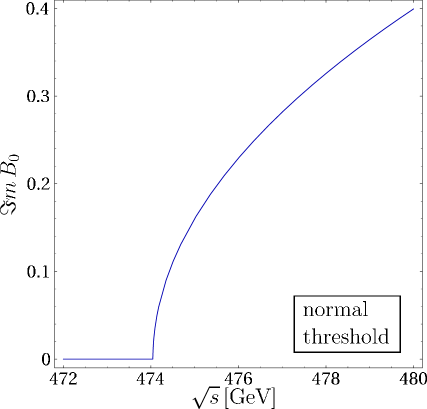
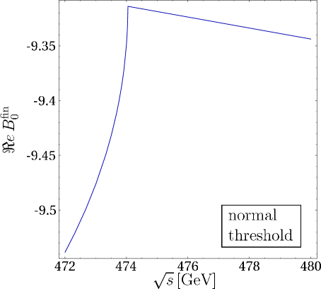
Figure 13: Effect of the normal threshold in the finite part of the 2-point function $B_{0}(s,m_{\tilde{\chi}^{0}_{1}}^{2},m_{\tilde{\chi}^{0}_{4}}^{2})$ at the branch cut $\sqrt{s_{\rm n}}=m_{\tilde{\chi}^{0}_{1}}+m_{\tilde{\chi}^{0}_{4}}=474.05$ GeV [in the SPS1a scenario].

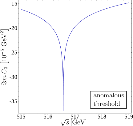
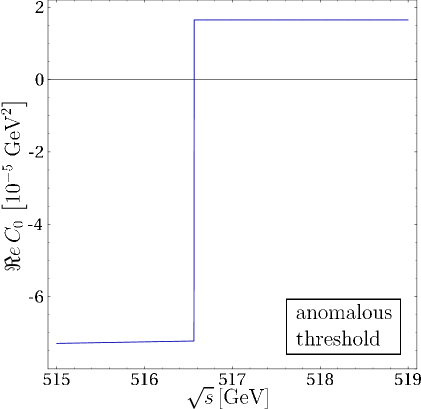
Figure 14: Effect of the anomalous threshold defined in eq. (88) in the 3-point function $C_{0}(s,m_{\tilde{\mu}}^{2},m_{\tilde{\mu}}^{2},m_{\tilde{\chi}^{0}_{1}}^{2},m_{\tilde{\chi}^{0}_{4}}^{2},0)$ at $\sqrt{s_{\rm a}}=516.56$ GeV [in the SPS1a scenario].

The two different types of threshold singularities for the vertex introduced above are exemplified in Fig. 13 and Fig. 14. The normal threshold singularity at $\sqrt{s_{\rm n}}$ in Fig. 13 is generated by the non-zero onset of the imaginary part of the 2-point function $B_{0}(s,m_{\tilde{\chi}^{0}_{1}}^{2},m_{\tilde{\chi}^{0}_{4}}^{2})$, corresponding to a kink in the real part. In contrast, the anomalous threshold at $\sqrt{s_{\rm a}}$ in Fig. 14 is generated by the $C_{0}(s,m_{\tilde{\mu}}^{2},m_{\tilde{\mu}}^{2},m_{\tilde{\chi}^{0}_{1}}^{2},m_{\tilde{\chi}^{0}_{4}}^{2},0)$ function, characterized by a kink in the imaginary part which leads, if integrated out in a dispersion relation, to a step in the real part [18].

4.4 Production Cross-Sections

Mediated by the pure s-channel $\gamma/Z$ exchange mechanisms, the production of smuon pairs is the most basic process of supersymmetric theories at $e^{+}e^{-}$ colliders. The results for the production cross-section will therefore be presented for this process first. Subsequently we expand the analysis to selectron pair production in $e^{+}e^{-}$ and $e^{-}e^{-}$ collisions which involve also t-channel neutralino exchange mechanisms. They will serve as an excellent instrument to measure the electron-selectron-gaugino SU(2) and U(1) Yukawa couplings, which will be analyzed at the end of this section.

4.4.1 Smuon production

After the renormalized transition amplitude for the process $e^{+}e^{-}\to{\tilde{\mu}}^{+}{\tilde{\mu}}^{-}$ is constructed following the way outlined in the last section, the experimental parameters must be defined properly. We use the on-shell definition for all masses, while the electromagnetic coupling $\alpha$ will be evaluated at the scale of the center-of-mass energy $Q=\sqrt{s}$, so that the large logarithmic corrections $\propto\log s/m_{f}^{2}$ from light fermion loops in the running of $\alpha(Q^{2})$ are absorbed into this definition.

The resulting amplitude is UV finite but still infrared divergent. This divergence is removed by adding the contributions from photon radiation in the initial and final states to the cross-section. The virtual and real QED corrections form a gauge invariant subset separate from the other virtual loop corrections.

Initial-state QED corrections: Adding to the loop-corrected cross-section the contribution of soft photon radiation from the initial lepton lines, the ensuing cross-section factorizes into the Born cross-section and a radiation coefficient that depends on the cut-off $\Delta E$ of the soft photon energy (defined in the cms frame),

$${\rm d}\sigma_{\rm ISR}^{\rm virt+soft}={\rm d}\sigma_{\rm Born}\,\frac{\alpha}{\pi}\left[\log\frac{(\Delta E)^{2}}{s}\left(\log\frac{s}{m_{\mathrm{e}}^{2}}-1\right)+\frac{3}{2}\,\log\frac{s}{m_{\mathrm{e}}^{2}}-2+\frac{\pi^{2}}{3}\right].$$ (90)

This $\Delta E$ dependence is removed if the radiation of hard photons is added to the cross-sections. We are still left, however, with the logarithmic enhancement of the cross-section from collinear radiation $\propto\log s/m_{\mathrm{e}}^{2}$. In leading logarithmic order the photon radiation effectively just reduces the cms energy available for the final-state particles [51]. This is described by the convolution

$${\rm d}\sigma_{\rm LL}(s)=\int_{4m_{\tilde{\mu}}^{2}/s}^{1}{\rm d}z\;\Gamma_{ee}^{\rm LL}(2\alpha,z,s)\,\sigma_{\rm Born}(zs)$$ (91)

of the Born cross-section with the radiator function [52]

$$\Gamma_{ee}^{\rm LL}(\alpha,z,Q^{2})=\delta(1-z)+\frac{\alpha}{2\pi}\,\log\frac{Q^{2}}{m_{\mathrm{e}}^{2}}\;\frac{1+z^{2}}{1-z}\Big{|}_{z\leq 1-\epsilon}$$ (92)

(that can easily be generalized to higher orders [53]). The variable $z$ denotes the energy fraction left to the electron/positron parton after the radiation of the collinear photon. The additional non-collinear photon radiation is treated numerically by applying Monte Carlo integration techniques, with fast convergence after the leading logarithmic order is subtracted analytically, as outlined above.

Final-state QED corrections: After adding up the vertex correction plus the final-state photon radiation, the cross-sections for soft photons factorizes again in the Born cross-section and a radiation function that depends on the photon cut-off energy $\Delta E$,

$${\rm d}\sigma_{\rm FSR}^{\rm virt+soft}={\rm d}\sigma_{\rm Born}\,\frac{\alpha}{\pi}\left\{\log\frac{4(\Delta E)^{2}}{m_{\tilde{\mu}}^{2}}\right. \left[-1+\frac{1+\beta^{2}}{2\beta}\log\frac{1+\beta}{1-\beta}\right]-2+\frac{1}{\beta}\log\frac{1+\beta}{1-\beta}$$ (93)

$$+\frac{1+\beta^{2}}{\beta} \left[\log\frac{1+\beta}{1-\beta}\left(1-\frac{1}{2}\log\frac{4\beta^{2}}{1-\beta^{2}}\right)\right.$$

$$\qquad\left.\left.+\frac{\pi^{2}}{3}+{\rm Li}_{2}\frac{1-\beta}{1+\beta}-{\rm Li}_{2}\frac{2\beta}{1+\beta}\right]\right\}.$$

Since the smuon mass is large, the velocity $\beta=(1-4m_{\tilde{\mu}}^{2}/s)^{1/2}$ of the smuons in the final state stays sufficiently away from unity not to generate collinear singularities. The $\Delta E$ dependence is neutralized when the hard photon contributions are added and integrated out (numerically) to calculate the total cross-section.

The initial and final-state QED corrections do not interfere in the total cross-section as a consequence of CP invariance. However, the amplitudes do in general interfere in the calculation of final-state distributions.

In general it is not possible to divide the virtual loop corrections for slepton pair production into SM-like corrections and genuine supersymmetric corrections. However, for the special case of ${\tilde{\mu}_{\rm R}}$ pair production, a gauge-invariant and UV-finite subset of SM-like loop contributions can be defined, including all diagrams where a SM fermion, gauge boson or the lightest Higgs boson is attached to the tree-level graphs, and taking the mixing angle $\alpha$ of the CP-even Higgs bosons to be $\alpha=\beta-\pi/2$. The remaining loop contributions can then be interpreted as the genuine virtual SUSY corrections. For this contribution we find relative corrections of the order of 1%, as demonstrated in Fig. 15, which nicely illustrates the onset of normal and anomalous thresholds in vertex and box diagrams with rising energy. The variation of the corrections across the $[M_{1},\mu]$ and $[M_{2},\mu]$ planes has been studied in Fig. 16 (a,b).

(a)

(b)

Figure 15: Corrections from genuine SUSY loops to the cross-section for $e^{+}e^{-}\to{\tilde{\mu}_{\rm R}}^{+}{\tilde{\mu}_{\rm R}}^{-}$ relative to the Born cross-section. The corrections are separated into vertex and self-energy corrections (a) and box corrections (b). The kinks are generated by normal (single arrows) and anomalous thresholds (double arrows). The values are given for the SPS1a scenario.

(a)

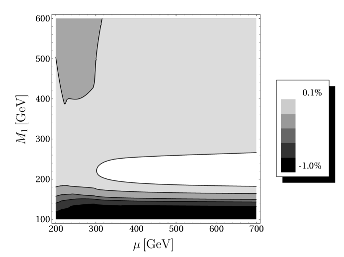
(b)

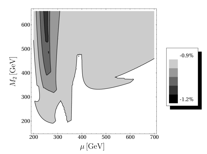
Figure 16: Dependence of the relative one-loop corrections $(\sigma_{\alpha}-\sigma_{\rm Born})/\sigma_{\rm Born}$ to ${\tilde{\mu}_{\rm R}}$ pair production on the gaugino parameters $M_{1}$, $M_{2}$ and $\mu$ for $\sqrt{s}=500$ GeV. The values of the other parameters are taken from the SPS1a scenario.

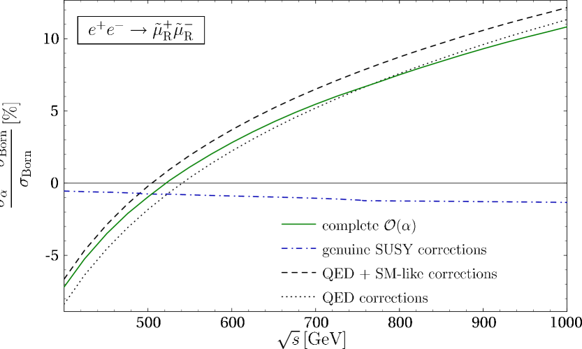
Figure 17: Electroweak corrections to the cross-section for $e^{+}e^{-}\to{\tilde{\mu}_{\rm R}}^{+}{\tilde{\mu}_{\rm R}}^{-}$, relative to the improved Born cross-section. Besides the full ${\mathcal{O}}(\alpha)$ result, contributions from different subsets of diagrams are shown. Input parameters taken from the SPS1a scenario.

All crucial elements have now been collected to present the overall correction of the total cross-section for ${\tilde{\mu}_{\rm R}}$ pair production. The parameters of the Snowmass reference point SPS1a have been adopted again to illustrate the final results. As a function of energy the correction normalized to the Born cross-section, defined for the running electromagnetic coupling, is displayed in Fig. 17. Moreover, the total correction is broken down to initial-state plus final-state QED corrections, the total SM corrections including just lines of SM particles in the virtual corrections, and the genuine SUSY corrections introduced above. The real photon radiation is treated in a fully inclusive way, i.e. both soft and hard photon emission are included. The main contribution to the corrections can trivially be traced back to the universal factorizable QED terms which are logarithmically enhanced. However, after these dominant effects are subtracted, the remaining QED, weak-loop and genuine SUSY contributions still amount to a level of 5%.

Thus precision measurements of the total cross-sections for slepton pair production, that may reach a level of a few per-mille, require the one-loop radiative corrections to be included properly. In this way a satisfactory understanding of the expected experimental results will be achieved.

4.4.2 Selectron production

In comparison to smuon pair production, the loop calculations to selectron pair production are significantly more complex, the reason being twofold. An extra technical challenge is introduced by the additional t-channel neutralino exchange mechanisms. These mechanisms also give rise to delicate problems for gauge invariant subdivisions of diagram classes and the subsequent renormalization procedures. The origin of the problems is the continuous flow of charges from the initial to the final states while, at the same time, the Fermi/Bose character of the charge line changes in the electron-selectron-neutralino Yukawa vertex—a SUSY vertex sui generis. Related problems were encountered first in $WW$ pair production via t-channel neutrino exchange as opposed to muon pair production in $e^{+}e^{-}$ collisions.

A transparent example is provided by the process $e_{\rm R}^{-}e_{\rm R}^{-}\to{\tilde{e}_{\rm R}}^{-}{\tilde{e}_{\rm R}}^{-}$ which is built up solely by t-channel neutralino exchanges:

1. Closed loops of leptons and sleptons implanted in the virtual neutralino lines form a gauge invariant subset of diagrams, and so do loops of quarks and squarks.

2. The diagrams involving massive gauge bosons, Higgs bosons, gauginos and higgsinos however cannot be separated from the QED loops in a gauge-invariant manner anymore. This follows from a simple argument. The set of photonic corrections to the electron-selectron-neutralino Yukawa vertex is not UV finite, but only so after being supplemented by the corresponding virtual photino diagram. Since the photino is not a mass eigenstate, this amplitude is closely linked to the remaining degrees of freedom in the electroweak sector. Thus only the total set of gauge boson/Higgs and gaugino/higgsino electroweak diagrams is gauge invariant.

   Nevertheless, as expected on general grounds, soft real-photon radiation regularizes the infrared divergences generated by the virtual photon diagrams, and the selectron pair cross-section for soft photon radiation factorizes again into the Born term times a radiator function. In leading logarithmic order of the soft-photon energy $\Delta E$,

   $$\rule{0.0pt}{0.0pt}{\rm d}\sigma_{\rm ISR+FSR}^{\rm virt+soft,log}={\rm d}\sigma_{\rm Born}\,\frac{\alpha}{\pi}\log\frac{(\Delta E)^{2}}{s}\left\{\log\frac{s}{m_{\mathrm{e}}^{2}}\right. +2\,\log 4\biggl{[}1+\log\frac{m_{\mathrm{e}}^{2}m_{\tilde{e}}^{2}}{(m_{\tilde{e}}^{2}-t)(m_{\tilde{e}}^{2}-u)}\biggr{]}$$ (94)

   $$+\left.\frac{1+\beta^{2}}{2\beta}\log\frac{1+\beta}{1-\beta}\right\},$$

   where $t$ and $u$ are the invariant momentum transfers in the t-/u-channel.

   In the same way, in leading logarithmic order, collinear photon radiation from the initial beam line can be cast in the convoluted form of eqs. (91), (92). Note however that virtual initial and final state radiation cannot (even not theoretically) be disentangled anymore.

The influence on parameters of the Higgs (and higgsino) sector is rather mild since the couplings of these fields to electron-type lines is negligible. Effects of Higgs bosons on the self-energies of the $Z$ boson and the neutralinos may naively be expected non-negligible. However, the leading effects of the Higgs boson spectrum on these parameters are only proportional to the logarithm of the mass ratios of two Higgs bosons, e.g. $\propto\log M_{\mathrm{A}}/M_{\mathrm{H}}$. As a result, these contributions are naturally suppressed.

(a)

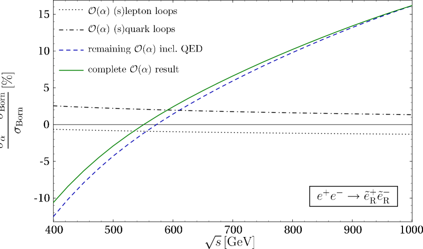
(b)

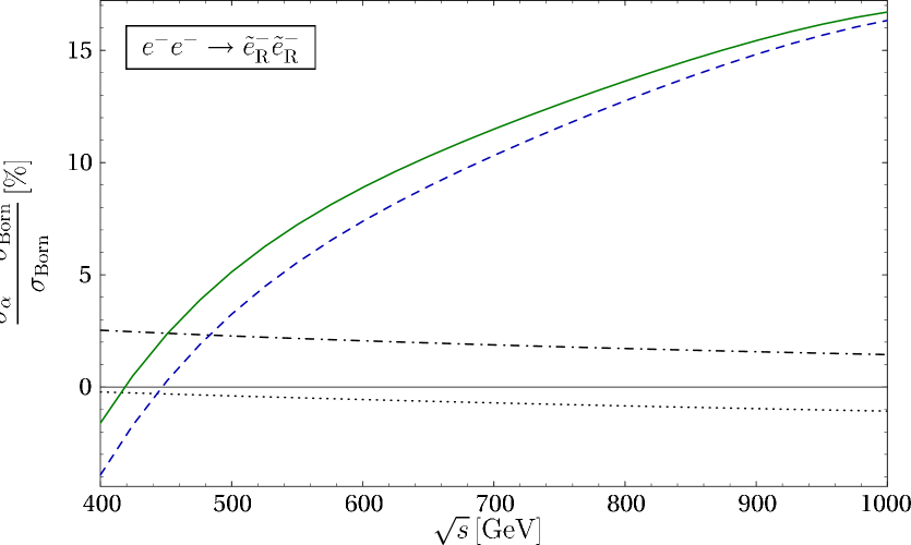
Figure 18: Electroweak corrections to the cross-sections (a) for $e^{+}e^{-}\to{\tilde{e}_{\rm R}}^{+}{\tilde{e}_{\rm R}}^{-}$ and (b) for $e^{-}e^{-}\to{\tilde{e}_{\rm R}}^{-}{\tilde{e}_{\rm R}}^{-}$, relative to the improved Born cross-section. Besides the full ${\mathcal{O}}(\alpha)$ result, contributions from different subsets of diagrams are shown. Input parameters taken from the SPS1a scenario.

The corrections to the RG improved Born cross-sections for selectron ${\tilde{e}_{\rm R}}$ pairs in $e^{+}e^{-}$ and $e^{-}e^{-}$ collisions are depicted in Fig. 18 (a) and (b). In addition to the full corrections, the results are broken down to the individual contributions from closed loops of leptons/sleptons, quarks/squarks and the remaining corrections involving gauge bosons, Higgs bosons, gauginos and higgsinos, as well as the QED corrections.

As before, we shall study the influence of the corrections induced through the supersymmetry sector at some detail. Even though the genuine SUSY loops are intimately correlated with the Standard Model loops, the higher-order effects vary widely over the supersymmetry parameter space, measuring the influence of the SUSY degrees of freedom beyond the trivial effects due to the masses and couplings of the selectrons produced in the final state.

(a)

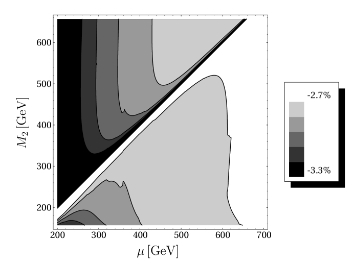
(b)

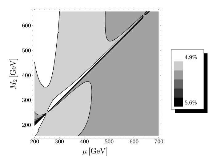
Figure 19: Dependence of the relative one-loop corrections $(\sigma_{\alpha}-\sigma_{\rm Born})/\sigma_{\rm Born}$ to ${\tilde{e}_{\rm R}}^{+}{\tilde{e}_{\rm R}}^{-}$ production (a) and ${\tilde{e}_{\rm R}}^{-}{\tilde{e}_{\rm R}}^{-}$ production (b) on the gaugino parameters $M_{2}$ and $\mu$ for $\sqrt{s}=500$ GeV. The values of the other parameters are taken from the SPS1a scenario.

A significant influence on the one-loop corrections arises from the electroweak gaugino sector, characterized by the parameters $M_{1}$, $M_{2}$ and $\mu$. As an example, the dependence of the one-loop corrections relative to the Born cross-section on $M_{2}$ and $\mu$ is shown in Figs. 19 (a) and (b). The effects are maximal for small $\mu$ due to the higgsino loops affecting the $W$ and $Z$ self-energies. [The rapid changes along the diagonal $M_{2}=\mu$ are a consequence of the level crossings between the $\tilde{\chi}^{0}_{i}$ states which induces drastic changes in the couplings to the electroweak gauge bosons.]

As outlined earlier, big mass differences between the SUSY sfermions and the corresponding SM fermions generate large effective Yukawa couplings and thus large superoblique corrections to selectron production. This can nicely be illustrated by comparing the squark loop effect on the smuon pair cross-sections with the selectron pair cross-section mediated by t-channel neutralino diagrams. Beyond the low-mass threshold region, the squark contributions are rising linearly in the logarithm of the squark masses for selectron production while approaching a plateau for smuon production, where gaugino/higgsino lines are absent at the Born level, cf. Figs. 20 (a) and (b).

(a)

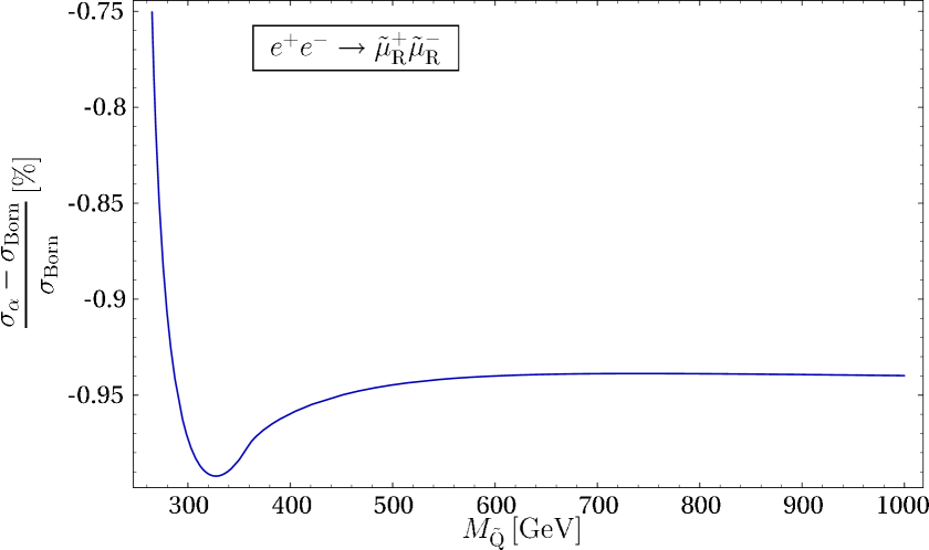
(b)

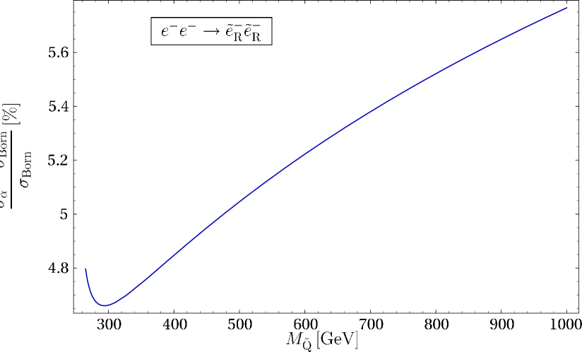
Figure 20: Dependence of the one-loop corrections on the soft-breaking squark mass parameter $M_{\rm\tilde{Q}}$ [assumed to be universal for all squarks] for (a) ${\tilde{\mu}_{\rm R}}^{+}{\tilde{\mu}_{\rm R}}^{-}$ production and (b) ${\tilde{e}_{\rm R}}^{-}{\tilde{e}_{\rm R}}^{-}$ production. The values of the other parameters are taken from the SPS1a scenario, and the cms energy is set to $\sqrt{s}=500$ GeV.

4.4.3 The identity of SUSY Yukawa and SM gauge couplings

Selectron-pair production in $e^{+}e^{-}$ collisions and, particularly, in $e^{-}e^{-}$ collisions are excellent channels for testing the identity of the SU(2) and U(1) SUSY Yukawa couplings and the corresponding SM gauge couplings. Selectron production in $e^{-}e^{-}$ collisions is mediated solely by neutralinos, and the same is true for initial-state leptons of equal helicities in $e^{+}e^{-}$ channels, as evident from Table 1.

Asymptotically, the t-channel exchange is the dominant mechanism. As a consequence of unitarity, the logarithmically leading part of the cross-section for high energies is independent of the neutralino mixing parameters after all neutralino exchanges in the t-channel are added up:

$$\sigma[e^{+}\,e^{-}\to{\tilde{e}_{\rm R}}^{+}\,{\tilde{e}_{\rm R}}^{-}] \stackrel{{\scriptstyle s\to\infty}}{{-\!\!\!\longrightarrow}}\frac{\hat{g}^{\prime 4}}{16\pi}\,\frac{\log s}{s}+{\mathcal{O}}\left(\frac{1}{s}\right),$$ (95)

$$\sigma[e^{+}\,e^{-}\to{\tilde{e}_{\rm L}}^{+}\,{\tilde{e}_{\rm L}}^{-}] \stackrel{{\scriptstyle s\to\infty}}{{-\!\!\!\longrightarrow}}\frac{(\hat{g}^{2}+\hat{g}^{\prime 2})^{2}}{16\pi}\,\frac{\log s}{s}+{\mathcal{O}}\left(\frac{1}{s}\right),$$ (96)

where $\hat{g}$ and $\hat{g}^{\prime}$ are the SU(2) and U(1) Yukawa couplings, respectively. However, very large energies indeed would be needed before the asymptotic behavior is reached in practice.

In this subsection we shall study the sensitivity of selectron production to the Yukawa electron-selectron-gaugino couplings and the errors expected experimentally. We assume that the masses and mixing parameters of the neutralinos have been pre-determined in chargino/neutralino pair-production, and we properly take into account the expected errors in this sector. It is important to note that the mixing parameters affecting the selectron production cross-sections depend only on the gaugino/higgsino mass parameters $M_{1}$, $M_{2}$ and $\mu$. These parameters can be determined in the MSSM from the precision measurements of three chargino and neutralino masses, for example, $\tilde{\chi}_{1}^{\pm}$, $\tilde{\chi}_{2}^{\pm}$ and $\tilde{\chi}^{0}_{1}$, but independently of the chargino/neutralino cross-sections [which would re-introduce the Yukawa couplings otherwise].

To derive the size of the errors on the Yukawa couplings, we perform this study in the one-loop approximation. Proper errors will be associated to all terms in the improved Born approximation. However, the higher-order corrections can be calculated for the ideal values of the parameters in the loops since their errors would affect the errors in the Yukawa couplings only to second order which is consistently neglected. Iterative procedures may later be employed for the next-level improvements.

The selectron production cross-sections are computed using the beam polarizations and cuts introduced in Section 3.3, and with beamstrahlung and ISR switched on. Besides enhancing the statistics, the polarization of both the $e^{-}$ and $e^{+}$ beams is essential for identifying the chiral quantum numbers of the selectrons [30]. Since only total cross-section measurements will be considered here, the one-loop corrections can be included by means of a simple K-factor. Besides the neutralino parameters, the cross-sections crucially depend on the selectron masses, which can be extracted from threshold scans, cf. Tab. 4. For the neutralino/chargino masses the following errors are assumed, $\delta m_{\tilde{\chi}^{0}_{1}}=50\,\,\mathrm{MeV}$, $m_{\tilde{\chi}^{0}_{2}}=80\,\,\mathrm{MeV}$, $\delta m_{\tilde{\chi}^{\pm}_{2}}=3000\,\,\mathrm{MeV}$, which are based on a coherent analysis of LHC and LC mass measurements [55]. From these masses, the gaugino and higgsino mass parameters can be derived, in models with two Higgs/higgsino doublets, to which we restrict our general analysis. These parameters determine the elements of the chargino and neutralino mixing matrices including estimates of their errors. An error of 1% is assigned to the polarization degree of the incoming electron/positron beams.

As discussed in Section 3, the L- and R-selectron states can be discriminated by considering the decay of the selectron ${\tilde{e}_{\rm L}}$ into the neutralino $\tilde{\chi}^{0}_{2}$, followed by the decay chain $\tilde{\chi}^{0}_{2}\to\tau^{+}\tau^{-}\,\tilde{\chi}^{0}_{1}$ and leading to the final states listed in Tab. 4. It is assumed that each tau pair can be identified with an efficiency of $\epsilon_{\tau}=80$%. In addition a global acceptance factor of $\epsilon_{\rm det}=50$% is assigned for potential detector effects, that are not simulated in this study.

(a) $e^{+}e^{-}$, $\sqrt{s}=500\,\,\mathrm{GeV}$, $L=500$ fb-1	(b) $e^{-}e^{-}$, $\sqrt{s}=500\,\,\mathrm{GeV}$, $L=50$ fb-1

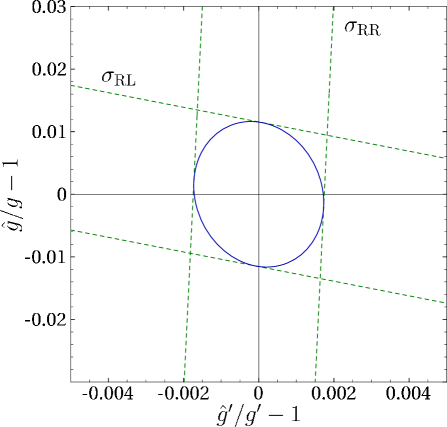
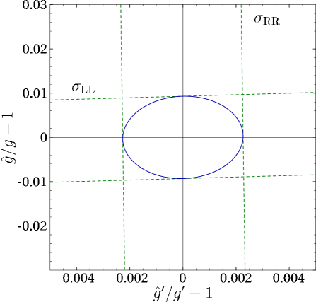
Figure 21: 1$\sigma$ bounds on the determination of the supersymmetric U(1) and SU(2) Yukawa couplings $\hat{g}^{\prime}$ and $\hat{g}$ from selectron cross-section measurements. The two plots compare the information obtained from the cross-sections $\sigma_{\rm RR}=\sigma[e^{+}\,e^{-}\to{\tilde{e}_{\rm R}}^{+}\,{\tilde{e}_{\rm R}}^{-}]$ and $\sigma_{\rm RL}=\sigma[e^{+}\,e^{-}\to{\tilde{e}_{\rm R}}^{\pm}\,{\tilde{e}_{\rm L}}^{\mp}]$ in the $e^{+}e^{-}$ mode (a) as well as $\sigma_{\rm RR}=\sigma[e^{-}\,e^{-}\to{\tilde{e}_{\rm R}}^{-}\,{\tilde{e}_{\rm R}}^{-}]$ and $\sigma_{\rm LL}=\sigma[e^{-}\,e^{-}\to{\tilde{e}_{\rm L}}^{-}\,{\tilde{e}_{\rm L}}^{-}]$ in the $e^{-}e^{-}$ mode (b), respectively. Parameters taken from the SPS1a scenario.

Taking into account all these statistical errors and systematic uncertainties, the constraints on the SU(2) and U(1) Yukawa couplings of the MSSM, $\hat{g}$ and $\hat{g}^{\prime}$, are presented in Fig. 21 (a) and (b) for the SPS1a scenario. The results are based on 500 fb^-1 data accumulated in $e^{+}e^{-}$ collisions at 500 GeV, and 50 fb^-1 in $e^{-}e^{-}$ collisions, respectively. From the overlap regions the following expected 1$\sigma$ errors are obtained:

$$e^{+}e^{-}: \frac{\delta\hat{g}^{\prime}}{\hat{g}^{\prime}} \approx 0.18\%, \frac{\delta\hat{g}}{\hat{g}} \approx 1.2\%,$$ (97)

$$e^{-}e^{-}: \frac{\delta\hat{g}^{\prime}}{\hat{g}^{\prime}} \approx 0.23\%, \frac{\delta\hat{g}}{\hat{g}} \approx 0.9\%.$$ (98)

As evident from these results, the expected sensitivity for the measurement of the Yukawa couplings in the $e^{+}e^{-}$ and $e^{-}e^{-}$ modes are similar. While $e^{-}$ polarization is essential for disentangling the SU(2) and U(1) couplings, the additional $e^{+}$ polarization reduces the errors by a factor of about 1.4 for a degree of 50%. The result for the determination of the U(1) bino Yukawa coupling is comparable to previous studies, Ref. [14, 54], while being slightly more precise than analyses based on the differential selectron cross-section [16].

The precision on the Yukawa couplings expected from selectron pair-production compares favorably with corresponding measurements in chargino/neutralino pair production, for which the errors are of similar though slightly larger magnitude [54, 10].

Thus it has turned out that one of the basic properties of supersymmetric theories, the identity of Yukawa and gauge couplings, can be tested with accuracies down to the per-cent and even per-mille level in selectron pair production at $e^{+}e^{-}$ and $e^{-}e^{-}$ colliders.

5 Conclusions

We have presented in this report the theoretical basis for high-precision studies of the supersymmetric partners to muons and electrons, the scalar smuons and selectrons, at future $e^{+}e^{-}$ and $e^{-}e^{-}$ linear colliders. The theoretical material elaborated in the study is complemented by phenomenological analyses of the masses and couplings of these particles.

Masses: A central target of experiments exploring the properties of supersymmetric particles is the measurement of their masses. The experimentally observed particle masses are connected with mass parameters in the SUSY Lagrangian that encode the breaking of supersymmetry and are thus directly related to the basic structure of the supersymmetric theory at the TeV scale. Extrapolating these parameters to high scales will allow us to reconstruct the fundamental supersymmetric theory.

Precision measurements can be performed in the clean environment of high-energy lepton colliders operating with polarized beams at high luminosity. The masses of scalar sleptons, selectrons in particular, can be determined with unparalleled precision from threshold scans as the excitation curves rise steeply with the energy above threshold, either with the third power in the velocity for smuons or even linearly for selectron channels.

As a consequence, accurate theoretical predictions for the pair production are required to match the expected experimental accuracies. The two theoretical key points in this context, non-zero width effects and Coulombic Sommerfeld rescattering effects, have been elaborated in detail. Special attention has been paid to preserving gauge invariance in truncated subsets of the entire ensemble of Feynman diagrams describing the final states after the resonance decays. The remaining contributions of this ensemble are taken into account as part of the SUSY backgrounds, with the additional backgrounds from SM sources added on.

Based on this procedure, a phenomenological analysis of slepton masses in threshold scans was performed, improving significantly on the theoretical reliability compared with earlier simulations. While the excitation curves are characterized by their distinct rise near the thresholds, including sub-dominant backgrounds reduces, somewhat, the precision expected from previous studies. Nevertheless, a precision of about a few 100 MeV can be expected for slepton masses around 200 GeV in general, corresponding to a relative error at the per-cent to per-mille level. For the R-selectron mass, an accuracy of even $0.2\times 10^{-3}$ can be obtained from threshold scans in the $e^{-}e^{-}$ mode, benefiting from the exceptionally sharp rise of the S-wave selectron excitation.

Moreover, the threshold scans of selectron pair production can also be exploited to extract the decay widths to accuracies between 10 and 20%.

Yukawa couplings: A key character of supersymmetric theories is the identity between the Yukawa couplings $\hat{g}(f\tilde{f}\widetilde{V})$ of the fermions, their superpartners and the gauginos, and the gauge couplings $g(ffV)/g(\tilde{f}\tilde{f}V)$ of the fermions and sfermions to the gauge bosons. The identity of these couplings is crucial for the natural solution of the fine-tuning problem. It must hold not only in theories with exact supersymmetry but also in theories incorporating the breaking of supersymmetry, as to ensure the stable extrapolation of the system to energies near the Planck scale—one of the defining raisons d’être for supersymmetry.

In passing it may be noticed that the identity of the gauge couplings themselves in the SM and SUSY sectors can be tested at the per-cent level. Smuon pair production is particularly suited for extracting the gauge couplings in the SUSY sector as this process is mediated solely by s-channel $\gamma$ and $Z$-boson exchanges.

In contrast, the SUSY Yukawa couplings of the electroweak sector may be probed in selectron pair production due to the neutralino t-channel exchange contribution. By carefully analyzing statistical errors and systematic uncertainties we could demonstrate that these couplings can be extracted from measurements of the total cross-sections in the high-energy continuum with a precision of better than the per-cent level. In particular, this slightly exceeds the accuracy that can be achieved by other methods, for example in the analysis of chargino/neutralino pair production.

Matching this expected experimental accuracy with its theoretical counterpart requires the calculation of the cross-sections to per-cent accuracy. For this purpose the complete next-to-leading order one-loop SUSY electroweak radiative corrections were calculated for the production of on-shell smuon and selectron pairs. The corrections were found to be sizable, being of the order of 5–10%, with genuine SUSY corrections accounting for about 1% in ${\tilde{\mu}_{\rm R}}$ pair production, where these corrections can be defined unambiguously and separated consistently.

In all examples analyzed in this report, the production of scalar electrons in $e^{+}e^{-}$ annihilation has been compared to the corresponding processes in $e^{-}e^{-}$ scattering. The $e^{-}e^{-}$ mode turns out to be particularly favorable for the measurement of the selectron masses in threshold scans. In addition it can provide complementary information on the selectron Yukawa couplings.

The detailed analytical expressions for the slepton pair production cross-sections are too lengthy to be reported here in writing. The results are implemented in computer programs that return the cross-sections for smuons and selectrons to one-loop order for whatever set of Lagrangian parameters in the Minimal Supersymmetric Standard Model MSSM is chosen. The computer codes are available from the web at http://theory.fnal.gov/people/afreitas/. [Technical information on installing and running the programs are given at the web site.]

The theoretical analysis presented in this report for smuons and selectrons is one of the cornerstones for precision analyses of the supersymmetry sector in particle physics. The precision that is expected to be achieved in future linear collider experiments requires the analysis of many different channels in parallel—sleptons, charginos/neutralinos and squarks/gluinos. The parameters of all these states affect mutually the theoretical predictions at the one-loop level so that all the associated production channels must be analyzed simultaneously. Such an overall analysis demands complementary and coherent experimental action at lepton and proton colliders—a program for which the present analysis is a crucial building block. This ensures finally a self-consistent picture of the SUSY sector at the phenomenological level.

Beyond drawing a high-resolution picture of supersymmetry at low energies, the precise determination of these parameters provides the base for exploring the mechanism of supersymmetry breaking and the reconstruction of the fundamental supersymmetric theory, potentially at scales near the Planck scale. In short, the high precision analyses provide us with a telescope for exploring the structure of physics at the scale of ultimate unification of genuine particle physics with gravity, as expected to be realized near the Planck scale.

Appendix

The theoretical results and the phenomenological analyses presented in this report, have been based on the specific reference scenario SPS1a for the MSSM, defined in the set of the “Snowmass Points and Slopes” [20].

The SPS1a point is a typical mSUGRA scenario characterized by fairly light sfermion masses. If realized in nature, a wealth of experimental information would become available on this supersymmetric theory from a linear collider operating in the first phase at energies up to about 1 TeV.

The SUSY parameters of SPS1a are defined at the GUT scale for the following universal values:

$$m_{0} =100\,\,\mathrm{GeV}, M_{1/2} =250\,\,\mathrm{GeV}, A_{0} =-100\,\,\mathrm{GeV}, \tan\beta =10, \mu >0.$$ (99)

The overall set is completed by the Standard Model parameters specified at the electroweak scale as

$$\alpha(M_{\mathrm{Z}}) =1/127.70, \qquad m_{\mathrm{t}} =175\,\,\mathrm{GeV},$$ (100)

$$M_{\mathrm{Z}} =91.1875\,\,\mathrm{GeV}, m_{\mathrm{b}} =4.25\,\,\mathrm{GeV},$$

$$M_{\mathrm{W}} =80.426\,\,\mathrm{GeV}, m_{\tau} =1.777\,\,\mathrm{GeV}.$$

The evolution of the soft SUSY breaking parameters (99) down to the electroweak scale by means of the program Isajet 7.58 leads to the weak-scale parameters listed in Ref. [24]. Uncertainties due to the implementation of the renormalization group evolution are not relevant for the purpose of the present study, since the MSSM parameters at the weak scale are taken as the starting point for our analysis. Using the MSSM soft-breaking parameters from Ref. [24] together with the SM parameters (100) the SUSY particles spectrum in Tab. 5 is obtained. The widths and branching ratios of the particles involved in the decay chains of the sleptons can be found in Tab. 2.

SUSY particles and masses

${\tilde{l}_{\rm R}}={\tilde{e}_{\rm R}}/{\tilde{\mu}_{\rm R}}$	$142.72$
${\tilde{l}_{\rm L}}={\tilde{e}_{\rm L}}/{\tilde{\mu}_{\rm L}}\,$	$202.32$
$\tilde{\nu}_{l}=\tilde{\nu}_{e}\,/\tilde{\nu}_{\mu}\>$	$185.99$
$\tilde{\tau}_{1}\,$	$132.97$
$\tilde{\tau}_{2}\,$	$206.29$
$\tilde{\nu}_{\tau}\,$	$185.05$

$\tilde{u}_{\mathrm{R}}$	$520.50$
$\tilde{u}_{\mathrm{L}}$	$537.20$
$\tilde{d}_{\mathrm{R}}$	$520.11$
$\tilde{d}_{\mathrm{L}}$	$543.07$

$\tilde{t}_{1}$	$375.74$
$\tilde{t}_{2}$	$585.15$
$\tilde{b}_{1}$	$488.01$
$\tilde{b}_{2}$	$528.23$

$\tilde{\chi}^{0}_{1}$	$96.18$
$\tilde{\chi}^{0}_{2}$	$176.62$
$\tilde{\chi}^{0}_{3}$	$358.80$
$\tilde{\chi}^{0}_{4}$	$377.87$
$\tilde{\chi}_{1}^{\pm}$	$176.06$
$\tilde{\chi}_{2}^{\pm}$	$378.51$

$h^{0}$	[89.28]0 122.71
$H^{0}$	[394.07] 393.56
$A^{0}$	[393.63] 393.63

Table 5: Mass spectrum in GeV of SUSY particles relevant for this study for the reference scenario SPS1a [20]. The Higgs masses are given in Born approximation [square brackets] and radiatively corrected.

The staus, squarks and Higgs bosons only enter in the loop corrections to smuon and selectron pair-production. The masses of the Higgs bosons in the loop contributions must be evaluated at tree level, in order to ensure the cancellation of gauge-parameter dependence in the next-to-leading order result. On the other hand, some of the background processes considered in Section 3.3 involve tree-level Higgs boson exchanges. In order to get reliable predictions for these processes, it is necessary to include the large radiative corrections to the Higgs masses, which for this purpose were calculated with the program FeynHiggs [57].

Added Note:

The SPS1a set of parameters generates the following predictions for the low-energy precision observables: BR$[b\to s\gamma]=2.7\cdot 10^{-4}$ and $\Delta(g_{\mu}-2)/2=17\cdot 10^{-10}$. The amount of cold dark matter is, with $\Omega_{\chi}h^{2}=0.18$, still compatible with WMAP data but somewhat on the high side if they are supplemented by the ACBAR and CBI data.

Shifting the scalar mass parameter slightly downwards to $m_{0}=70$ GeV, but not altering any of the other universal parameters in SPS1a, drives the value for the density of cold dark matter to the central band of the data, $\Omega_{\chi}h^{2}=0.126$, without violating the bounds on BR$[b\to s\gamma]$ and $\Delta(g_{\mu}-2)/2$ [58]. Slepton, chargino/neutralino masses and branching ratios relevant for the present analysis change within so limited a margin that none of the conclusions in this report is affected to a significant amount.

References

• [1] J. Wess and B. Zumino, Nucl. Phys. B 70 (1974) 39.
• [2] H. P. Nilles, Phys. Rept.  110 (1984) 1;
H. E. Haber and G. L. Kane, Phys. Rept.  117 (1985) 75.
• [3] E. Witten, Phys. Lett. B 105 (1981) 267.
• [4] J. R. Ellis, S. Kelley and D. V. Nanopoulos, Phys. Lett. B 249 (1990) 441;
U. Amaldi, W. de Boer and H. Fürstenau, Phys. Lett. B 260 (1991) 447;
P. Langacker and M. X. Luo, Phys. Rev. D 44 (1991) 817.
• [5] G. A. Blair, W. Porod and P. M. Zerwas, Phys. Rev. D 63 (2001) 017703;
G. A. Blair, W. Porod and P. M. Zerwas, Eur. Phys. J. C 27 (2003) 263;
P. M. Zerwas et al., in Proc. of the 31st International Conference on High Energy Physics (ICHEP 2002), eds. S. Bentvelsen, P. de Jong, J. Koch and E. Laenen, Amsterdam, The Netherlands (2002) [hep-ph/0211076].
• [6] E. Accomando et al., Phys. Rept.  299 (1998) 1;
T. Behnke, J. D. Wells and P. M. Zerwas, Prog. Part. Nucl. Phys.  48 (2002) 363.
• [7] Tesla Technical Design Report, Part III, eds. R. Heuer, D. J. Miller, F. Richard and P. M. Zerwas, DESY-2001-11C [hep-ph/0106315].
• [8] T. Abe et al. [American Linear Collider Working Group Collaboration], in Proc. of the APS/DPF/DPB Summer Study on the Future of Particle Physics (Snowmass 2001), eds. R. Davidson and C. Quigg, SLAC-R-570 [hep-ex/0106056];
K. Abe et al. [ACFA Linear Collider Working Group Collaboration], KEK-REPORT-2001-11 [hep-ph/0109166].
• [9] G. Guignard (ed.), A 3-TeV $e^{+}e^{-}$ linear collider based on CLIC technology, CERN-2000-008.
• [10] S. Y. Choi, A. Djouadi, M. Guchait, J. Kalinowski, H. S. Song and P. M. Zerwas, Eur. Phys. J. C 14 (2000) 535;
S. Y. Choi, J. Kalinowski, G. Moortgat-Pick and P. M. Zerwas, Eur. Phys. J. C 22 (2001) 563.
• [11] M. A. Diaz, S. F. King and D. A. Ross, Nucl. Phys. B 529 (1998) 23;
S. Kiyoura, M. M. Nojiri, D. M. Pierce and Y. Yamada, Phys. Rev. D 58 (1998) 075002;
T. Blank and W. Hollik, in Proc. of the 2nd ECFA/DESY Linear Collider Study (2000) pp. 1248–1260, LC-TH-2000-054 [hep-ph/0011092].
• [12] A. Freitas et al., in Proc. of the 31st International Conference on High Energy Physics (ICHEP 2002), eds. S. Bentvelsen, P. de Jong, J. Koch and E. Laenen, Amsterdam, The Netherlands (2002) [hep-ph/0211108];
J. Kalinowski, to appear in the Proc. of the Extended ECFA/DESY Linear Collider Study (2003) [hep-ph/0309235].
• [13] J. L. Feng, Int. J. Mod. Phys. A 13 (1998) 2319;
J. L. Feng and M. E. Peskin, Phys. Rev. D 64 (2001) 115002;
see also C. A. Heusch, in Proc. of the 5th International Linear Collider Workshop (LCWS 2000), Fermilab, Batavia, Illinois (2000).
• [14] J. L. Feng, M. E. Peskin, H. Murayama and X. Tata, Phys. Rev. D 52 (1995) 1418.
• [15] A. Freitas, D. J. Miller and P. M. Zerwas, Eur. Phys. J. C 21 (2001) 361.
• [16] M. M. Nojiri, K. Fujii and T. Tsukamoto, Phys. Rev. D 54 (1996) 6756.
• [17] H. C. Cheng, J. L. Feng and N. Polonsky, Phys. Rev. D 56 (1997) 6875;
M. M. Nojiri, D. M. Pierce and Y. Yamada, Phys. Rev. D 57 (1998) 1539;
E. Katz, L. Randall and S. Su, Nucl. Phys. B 536 (1998) 3.
• [18] R. Karplus, C. M. Sommerfield and E. H. Wichmann, Phys. Rev.  111 (1958) 1187;
Y. Nambu, Nuovo Cim.  9 (1958) 610;
L. D. Landau, Nucl. Phys.  13 (1959) 181.
• [19] J. D. Bjorken and S. D. Drell, Relativistic Quantum Field Theory, McGraw-Hill, New York (1965).
• [20] B. C. Allanach et al., Eur. Phys. J. C 25 (2002) 113.
• [21] H. U. Martyn and G. A. Blair, in Proc. of the International Workshop on Linear Colliders, Sitges, Spain (1999) [hep-ph/9910416];
H. U. Martyn, contribution to Workshop on Physics at TeV Colliders, Les Houches, France (1999) [hep-ph/0002290].
• [22] A. Freitas and A. v. Manteuffel, in Proc. of the 10th International Conference on Supersymmetry and Unification of Fundamental Interactions (SUSY02), eds. P. Nath and P. M. Zerwas, Hamburg, Germany (2002) [hep-ph/0211105].
• [23] A. Freitas, Ph.D. thesis, Hamburg (2002), DESY-THESIS-2002-023;
A. v. Manteuffel, Diploma thesis, Hamburg (2003).
• [24] N. Ghodbane and H. U. Martyn, in Proc. of the APS/DPF/DPB Summer Study on the Future of Particle Physics (Snowmass 2001) ed. R. Davidson and C. Quigg [hep-ph/0201233].
• [25] A. Sommerfeld, Atombau und Spektrallinien, Bd. 2, (Vieweg, Braunschweig, 1939);
A. D. Sakharov, Zh. Eksp. Teor. Fiz.  18 (1948) 631 [Sov. Phys. Usp.  34 (1991) 375].
• [26] V. S. Fadin and V. A. Khoze, JETP Lett.  46 (1987) 525;
V. S. Fadin and V. A. Khoze, Sov. J. Nucl. Phys.  48 (1988) 309;
V. S. Fadin, V. A. Khoze and A. D. Martin, Phys. Lett. B 320 (1994) 141.
• [27] D. Y. Bardin, W. Beenakker and A. Denner, Phys. Lett. B 317 (1993) 213;
V. S. Fadin, V. A. Khoze, A. D. Martin and A. Chapovsky, Phys. Rev. D 52 (1995) 1377.
• [28] H.-U. Martyn, in Conceptual Design of a 500 GeV $e^{+}e^{-}$ Linear Collider, eds. R. Brinkmann, G. Materlik, J. Rossbach and A. Wagner, DESY 1997-048 and ECFA 1997-182.
• [29] V. D. Barger and T. Han, Phys. Lett. B 212 (1988) 117;
V. D. Barger, T. Han and R. J. Phillips, Phys. Rev. D 39 (1989) 146;
A. Tofighi-Niaki and J. F. Gunion, Phys. Rev. D 39 (1989) 720.
• [30] G. Moortgat-Pick et al., in Proc. of the 31st International Conference on High Energy Physics (ICHEP 2002), eds. S. Bentvelsen, P. de Jong, J. Koch and E. Laenen, Amsterdam, The Netherlands (2002) [hep-ph/0210212].
• [31] E. A. Kuraev and V. S. Fadin, Sov. J. Nucl. Phys.  41 (1985) 466 ;
G. Altarelli and G. Martinelli, in Physics at LEP, eds. J. Ellis and R. Peccei (CERN-86-02), Vol. 1, p. 47.
• [32] T. Ohl, Comput. Phys. Commun.  101 (1997) 269.
• [33] JLC Collaboration, KEK Report KEK-92-16 (1992);
T. Tsukamoto, K. Fujii, H. Murayama, M. Yamaguchi and Y. Okada, Phys. Rev. D 51 (1995) 3153.;
M. Dima et al., Phys. Rev. D 65 (2002) 071701.
• [34] W. Siegel, Phys. Lett. B 84 (1979) 193;
D. M. Capper, D. R. Jones and P. van Nieuwenhuizen, Nucl. Phys. B 167 (1980) 479.
• [35] W. Hollik, E. Kraus, M. Roth, C. Rupp, K. Sibold and D. Stöckinger, Nucl. Phys. B 639 (2002) 3;
W. Majerotto, in Proc. of the 10th International Conference on Supersymmetry and Unification of Fundamental Interactions (SUSY02), eds. P. Nath and P. M. Zerwas, Hamburg, Germany (2002) [hep-ph/0209137].
• [36] J. Küblbeck, M. Böhm and A. Denner, Comput. Phys. Commun.  60 (1990) 165;
T. Hahn, Comput. Phys. Commun.  140 (2001) 418;
T. Hahn and C. Schappacher, Comput. Phys. Commun.  143 (2002) 54;
T. Hahn, FeynArts 3 User’s Guide (2001) [http://www.feynarts.de].
• [37] R. Mertig, M. Böhm and A. Denner, Comput. Phys. Commun.  64 (1991) 345.
• [38] G. ’t Hooft and M. J. Veltman, Nucl. Phys. B 153 (1979) 365.
• [39] G. J. van Oldenborgh and J. A. Vermaseren, Z. Phys. C 46 (1990) 425;
T. Hahn and M. Pérez-Victoria, Comput. Phys. Commun.  118 (1999) 153;
T. Hahn, LoopTools 2 User’s Guide (2001) [http://www.feynarts.de/looptools].
• [40] A. Denner, Fortsch. Phys.  41 (1993) 307.
• [41] D. Pierce and A. Papadopoulos, Phys. Rev. D 50 (1994) 565;
D. Pierce and A. Papadopoulos, Nucl. Phys. B 430 (1994) 278;
T. Fritzsche and W. Hollik, Eur. Phys. J. C 24 (2002) 619.
• [42] H. Eberl, M. Kincel, W. Majerotto and Y. Yamada, Phys. Rev. D 64 (2001) 115013;
W. Öller, H. Eberl, W. Majerotto and C. Weber, Eur. Phys. J. C 29 (2003) 563.
• [43] A. Freitas and D. Stöckinger, Phys. Rev. D 66 (2002) 095014.
• [44] P. Chankowski, S. Pokorski and J. Rosiek, Nucl. Phys. B 423 (1994) 437;
A. Dabelstein, Z. Phys. C 67 (1995) 495;
L. H. Wan, W. G. Ma, R. Y. Zhang and J. Yi, Phys. Rev. D 64 (2001) 115004.
• [45] J. A. Coarasa, D. Garcia, J. Guasch, R. A. Jiménez and J. Solà, Eur. Phys. J. C 2 (1998) 373.
• [46] J. Gunion, T. Han, J. Jiang and A. Sopczak, Phys. Lett. B 565 (2003) 42.
• [47] E. Boos, H. U. Martyn, G. Moortgat-Pick, M. Sachwitz, A. Sherstnev and P. M. Zerwas, Eur. Phys. J. C 30 (2003) 395.
• [48] K. Symanzik, Commun. Math. Phys.  34 (1973) 7;
T. Appelquist and J. Carazzone, Phys. Rev. D 11 (1975) 2856.
• [49] M. J. Veltman, Nucl. Phys. B 123 (1977) 89.
• [50] R. Barbieri and G. F. Giudice, Nucl. Phys. B 306 (1988) 63;
M. Drees and S. P. Martin, in Electroweak symmetry breaking and new physics at the TeV scale, eds. T. L. Barklow, S. Dawson, H. E. Haber and J. L. Siegrist (1995), pp. 146–215 [hep-ph/9504324];
K. L. Chan, U. Chattopadhyay and P. Nath, Phys. Rev. D 58 (1998) 096004;
J. L. Feng, K. T. Matchev and T. Moroi, Phys. Rev. Lett.  84 (2000) 2322;
J. L. Feng, K. T. Matchev and T. Moroi, Phys. Rev. D 61 (2000) 075005.
• [51] M. S. Chen and P. M. Zerwas, Phys. Rev. D 11 (1975) 58.
• [52] E. A. Kuraev and V. S. Fadin, Sov. J. Nucl. Phys.  41 (1985) 466;
G. Altarelli and G. Martinelli, in Physics at LEP, eds. J. Ellis and R. Peccei (CERN-86-02), Vol. 1, p. 47.
• [53] M. Skrzypek and S. Jadach, Z. Phys. C 49 (1991) 577;
M. Skrzypek, Acta Phys. Polon. B 23 (1992) 135;
M. Cacciari, A. Deandrea, G. Montagna and O. Nicrosini, Europhys. Lett.  17 (1992) 123.
• [54] H. C. Cheng, J. L. Feng and N. Polonsky, Phys. Rev. D 57 (1998) 152.
• [55] LHC/LC Study Group Working Report, in preparation.
• [56] SPA Project of the SUSY Working Group within the ECFA Linear Collider Study 2003/04, in progress.
• [57] S. Heinemeyer, W. Hollik and G. Weiglein, Comput. Phys. Commun.  124 (2000) 76.
• [58] A. Belyaev (private communication);
see also H. Baer, C. Balazs, A. Belyaev, T. Krupovnickas and X. Tata, JHEP 0306 (2003) 054.