$B$-decays and $B-\overline{B}$ mixing within a heavy-light chiral quark model

Abstract

We describe a recently developed heavy-light chiral quark model and show how it can be used to calculate decay amplitudes for heavy mesons. In particular, we discuss $B\,-\,\overline{B}$ mixing, $B\rightarrow D\bar{D}$, $B\rightarrow D\eta^{\prime}$ and the beta term for $D^{*}\rightarrow D\gamma$.

1 Introduction

Some $B$-decays where the energy release is big compared to the light meson masses, for instance $B\rightarrow\pi\pi$ and $B\rightarrow K\pi$, has been successfully described by QCD factorization [1, 2]. However, for various $B$-decays where the energy release is of order 1 GeV or less , QCD factorization is not expected to hold. The purpose of this presentation is to describe how processes like $B\,-\,\overline{B}$ mixing [3], $B\rightarrow D\bar{D}$ [4], $B\rightarrow D\eta^{\prime}$ [5], and in addition, some aspects of $D$-meson decays [6, 7] can be described within a recently developed heavy-light chiral quark model (HL$\chi$QM) [8].

In general, weak non-leptonic processes may be described by an effective Lagrangian which is a linear combination of quark operators where the (Wilson) coefficients are calculated in perturbation theory. These quark operators are bosonized within the HL$\chi$QM, where non-factorizable effects can be incorporated by means of gluon condensates and chiral loops. The coefficients of the various terms of weak chiral Lagrangians can then be calculated. In this way we can make a bridge between the quark and the mesonic sector.

2 The heavy-light chiral quark model

Our model is based on the following Lagrangian containing both quark and meson fields:

$${\cal L}={\cal L}_{HQEFT}+{\cal L}_{\chi QM}+{\cal L}_{Int}\;,$$ (1)

where [9]

$${\cal L}_{HQEFT}=\overline{Q_{v}}\,iv\cdot D\,Q_{v}+{\cal L}_{HQEFT}^{(1)}+{\cal O}(m_{Q}^{-2})$$ (2)

is the Lagrangian for heavy quark effective field theory (HQEFT). The heavy quark field $Q_{v}$ annihilates a heavy quark with velocity $v$ and mass $m_{Q}$. Moreover, $D_{\mu}$ is the covariant derivative containing the gluon field (eventually also the photon field). The first order ($m_{Q}^{-1}$) term is

$${\cal L}_{HQEFT}^{(1)}=\frac{1}{2m_{Q}}\overline{Q_{v}}\,\left(-C_{M}\frac{g_{s}}{2}\sigma\cdot G\,+\,(iD_{\perp})_{\text{eff}}^{2}\right)\,Q_{v}\;,$$ (3)

where $\sigma\cdot G=\sigma^{\mu\nu}G^{a}_{\mu\nu}t^{a}$, and $\sigma^{\mu\nu}=i[\gamma^{\mu},\gamma^{\nu}]/2$. $G^{a}_{\mu\nu}$ is the gluonic field tensor, and $t^{a}$ are the colour matrices ($a=$1,..8). This chromo-magnetic term has a factor $C_{M}$, being one at tree level, but slightly modified by perturbative QCD. (When the covariant derivative also contains the photon field, there is also a corresponding magnetic term $\sim\sigma\cdot F$, where $F^{\mu\nu}$ is the electromagnetic tensor). Furthermore, $(iD_{\perp})_{\text{eff}}^{2}=C_{D}(iD)^{2}-C_{K}(iv\cdot D)^{2}$. At tree level, $C_{D}=C_{K}=1$. Here, $C_{K}$ is different from one due to perturbative QCD, while $C_{D}$ is not modified [10].

The light quark sector is described by the chiral quark model ($\chi$QM), having a standard QCD term and a term describing interactions between quarks and (Goldstone) mesons [11]. Making a flavour rotation of the quark fields $q_{L}$ and $q_{R}$ transforming as $SU(3)_{L}$ and $SU(3)_{R}$ respectively, the Lagrangian can be written in terms of quark fields $\chi$ transforming as $SU(3)_{V}$ triplets (see refs.[11, 12, 13, 14] and references therein):

$${\cal L}_{\chi QM}=\overline{\chi}\left[\gamma^{\mu}(iD_{\mu}+{\cal V}_{\mu}+\gamma_{5}{\cal A}_{\mu})-m\right]\chi-\overline{\chi}\widetilde{M_{q}}\chi\;,$$ (4)

where $\chi_{L}=\xi^{\dagger}q_{L}$ and $\chi_{R}=\xi q_{R}$. Here, $\xi=\exp(i\Pi/f)$, where $\Pi$ is a 3 by 3 matrix containing the (would be) Goldstone octet ($\pi,K,\eta$) in the standard way, and $f$ is the bare pion decay constant. The quantity $m$ is the ($SU(3)$ - invariant) constituent quark mass for light quarks. The vector and axial vector fields ${\cal V}_{\mu}$ and ${\cal A}_{\mu}$ are given by:

$${\cal V}_{\mu}=\frac{i}{2}(\xi^{\dagger}\partial_{\mu}\xi+\xi\partial_{\mu}\xi^{\dagger})\;\;;\;\;{\cal A}_{\mu}=-\frac{i}{2}(\xi^{\dagger}\partial_{\mu}\xi-\xi\partial_{\mu}\xi^{\dagger})\;,$$ (5)

and $\widetilde{M_{q}}$ defines the rotated version of the current light mass matrix ${\cal M}_{q}=diag(m_{u},m_{d},m_{s})$:

$$\widetilde{M_{q}}=\widetilde{M}_{q}^{V}+\widetilde{M}_{q}^{A}\gamma_{5}\;\;;\quad\widetilde{M}_{q}^{V,A}\,\equiv\,\frac{1}{2}(\xi^{\dagger}{\cal M}_{q}\xi^{\dagger}\,\pm\,\xi{\cal M}_{q}^{\dagger}\xi)\;.$$ (6)

In the light sector, the various pieces of the strong chiral Lagrangian can be obtained by integrating out the constituent quark fields $\chi$, and these pieces can be written in terms of the fields ${\cal A}_{\mu}\,,\,\widetilde{M}_{q}^{V}$ and $\widetilde{M}_{q}^{A}$.

In the heavy-light case, the generalization of the meson - quark interactions in the pure light sector $\chi$QM is given by the following $SU(3)_{V}$ invariant Lagrangian [8, 15, 16]:

$${\cal L}_{Int}=-G_{H}\,\left[\overline{\chi}_{k}\,\overline{H_{v}^{k}}\,Q_{v}\,+\overline{Q_{v}}\,H_{v}^{k}\,\chi_{k}\right]\;,$$ (7)

where $G_{H}$ is a coupling constant, and $H_{v}^{k}$ is the heavy meson field containing a spin zero and spin one boson:

$$H_{v}^{k} =P_{+}(P_{\mu}^{k}\gamma^{\mu}-iP_{5}^{k}\gamma_{5})\;,$$ (8)

$$\overline{H_{v}^{k}} =\gamma^{0}(H_{v}^{k})^{\dagger}\gamma^{0}\;;\quad P_{\pm}=(1\pm\gamma\cdot v)/2\;.$$

Here the index $k$ runs over the light quark flavours $u,d,s$. The fields $P_{5}(P_{\mu})$ annihilates a heavy-light meson with spin-parity $0^{-}(1^{-})$, and velocity $v$. Note that for antiquarks, the heavy quark field $Q_{v}{\,\equiv\,}Q_{v}^{(+)}$ has to be replaced by the heavy $anti$quark field $Q_{v}^{(-)}$ in (2) and (7). At the same time, the heavy meson field $H_{v}{\,\equiv\,}H_{v}^{(+)}$ in (7) and (8) has to be replaced by the $anti$meson field $H_{v}^{(-)}$, and the velocity $v$ is replaced by $(-v)$.

In our model, the hard gluons are thought to be integrated out and we are left with soft gluonic degrees of freedom. Emission of such gluons can be described using external field techniques [17], and their effect will be parameterized by vacuum expectation values, i.e. the gluon condensate ${\langle}\frac{\alpha_{s}}{\pi}G^{2}{\rangle}$. Our model dependent gluon condensate contributions are obtained by the replacement

$$g_{s}^{2}G_{\mu\nu}^{a}G_{\alpha\beta}^{b}\;\rightarrow\frac{4\pi^{2}\delta^{ab}}{(N_{c}^{2}-1)}{\langle}\frac{\alpha_{s}}{\pi}G^{2}{\rangle}\frac{1}{12}(g_{\mu\alpha}g_{\nu\beta}-g_{\mu\beta}g_{\nu\alpha})\,.$$ (9)

We observe that soft gluons coupling to a heavy quark is suppressed by $1/m_{Q}$, since to leading order the vertex is proportional to $v_{\mu}v_{\nu}G^{a\mu\nu}=0$, $v_{\mu}$ being the heavy quark velocity.

Note that opposite parity heavy meson states, like the recently discovered $D^{*}$ resonance, can also be incorporated in the formalism [18].

3 Bosonization within the HL$\chi$QM

The interaction term ${\cal{L}}_{Int}$ in (7) can now be used to bosonize the model, i.e. integrate out the quark fields. This can be done in the path integral formalism, or in terms of Feynman diagrams by attaching the external fields $H_{v}^{k},\overline{H_{v}^{k}},{\cal{V}}^{\mu},{\cal{A}}^{\mu}$ and $\widetilde{M}_{q}^{V,A}$ of section 2 to quark loops. Some of the loop integrals will be divergent and have to be related to physical parameters, as for the pure light sector [11, 12, 13, 14]. The strong chiral Lagrangian has the following form (see [8, 19] and references therein):

$${\cal L}_{Str}=\,-Tr\left[\overline{H_{k}}(iv\cdot D)H_{k}\right]\,+\,Tr\left[\overline{H_{k}}H_{h}v_{\mu}{\cal V}^{\mu}_{hk}\right]$$

$$-\,g_{\cal A}Tr\left[\overline{H_{k}}H_{h}\gamma_{\mu}\gamma_{5}{\cal A}^{\mu}_{hk}\right]+2\lambda_{1}Tr\left[\overline{H_{k}}H_{h}(\widetilde{M}_{q}^{V})_{hk}\right]+...$$ (10)

where the velocity index on the heavy meson field is suppressed, the ellipses indicate other terms (of higher order, say), and $D_{\mu}$ contains the photon field. The trace runs over gamma matrices.

Comparing the loop integral for the diagrams in figure 1 with the vector field ${\cal V}_{\mu}$ attached to the light quark, we obtain the following identification:

$$-iG_{H}^{2}N_{c}\,(I_{3/2}+2mI_{2}+\frac{i(8-3\pi)}{384N_{c}m^{3}}{\langle}\frac{\alpha_{s}}{\pi}G^{2}{\rangle})=1\;,$$ (11)

where $I_{3/2}$ and $I_{2}$ are linear - and logarithmic - divergent loop integrals (these have to be interpreted as the regularized ones). Note that for the kinetic term in (10) we obtain the same relation as (11) due to the relevant Ward identity.

The relation (11) is analogous to the pure light sector where the quadratic and logarithmic divergent integrals are related to $f$ (the bare $f_{\pi}$) and the quark condensate [11, 12, 13, 14]:

$$f^{2}=-i4m^{2}N_{c}I_{2}+\frac{1}{24m^{2}}{\langle}\frac{\alpha_{s}}{\pi}G^{2}{\rangle}\;,$$ (12)

$${\langle}\,\overline{q}q\,{\rangle}=-4imN_{c}I_{1}-\frac{1}{12m}{\langle}\frac{\alpha_{s}}{\pi}G^{2}{\rangle}\;,$$ (13)

where $I_{1}$ is the quadratically divergent loop integral. As the pure light sector is a part of our model, we have to keep these relations in the heavy-light case studied here.

Also from diagram 1, with the axial field ${\cal A}_{\mu}$ attached, we obtain a similar identification for the axial vector coupling $g_{\cal A}$. Using (11) this can be rewritten:

Figure 1: Diagrams contributing to the lowest order heavy-light chiral Lagrangian.

$$g_{\cal A}=1+\frac{4}{3}iG_{H}^{2}N_{c}\,\left(I_{3/2}-\frac{im}{16\pi}\right)\;.$$ (14)

Within a primitive cut-off regularization, $I_{3/2}$ is (in the leading approximation) proportional to the cut-off in first power [15], while it is finite in dimensional regularization. We will keep $I_{3/2}$ as a free parameter to be determined by the physical value of $g_{\cal A}$.

Within HQEFT the weak current will, below the renormalization scale $\mu=m_{Q}\,(=m_{b},m_{c})$, be modified in the following way:

$$J_{k}^{\alpha}={\overline{\chi}}_{h}\xi^{\dagger}_{hk}\Gamma^{\alpha}Q_{v}\,+{\cal O}(m_{Q}^{-1})\;,$$ (15)

where $k$ and $h$ are light flavour indices. The $1/m_{Q}$ terms contain an extra covariant derivative [9] and

$$\Gamma^{\alpha}\,{\,\equiv\,}\,C_{\gamma}(\mu)\,\gamma^{\alpha}\,L\,+\,C_{v}(\mu)\,v^{\alpha}\,R\;,$$ (16)

where $L$ and $R$ are left and right Dirac projection matrices. The coefficients $C_{\gamma,v}(\mu)$ are determined by QCD renormalization for $\mu<m_{Q}$ and have been calculated to NLO.

Figure 2: Diagrams for bosonization of the heavy-light left handed quark current.

We obtain to zero order in the axial field ${\cal A}^{\mu}$ (-or ${\cal O}(p^{0})$ in the language of chiral perturbation theory. See figure 2):

$$J_{k}^{\alpha}(0)=\frac{\alpha_{H}}{2}Tr\left[\xi^{\dagger}_{hk}\Gamma^{\alpha}H_{vh}\right]\;,$$ (17)

where

$$\alpha_{H}{\,\equiv\,}-2iG_{H}N_{c}\left(-I_{1}+mI_{3/2}+\frac{i(3\pi-4)}{384m^{2}N_{c}}{\langle}\frac{\alpha_{s}}{\pi}G^{2}{\rangle}\right)\;.$$ (18)

We observe that, as this relation involves $I_{1}$, there is a relation between $\alpha_{H}$ and the quark condensate [8].

The coupling $\alpha_{H}$ in (17) is related to the physical decay constant $f_{H}$ by considering (for $H=B,D$):

$${\langle}0|\overline{u}\gamma^{\alpha}\gamma_{5}b|H{\rangle}= -2\,{\langle}0|J_{a}^{\alpha}|H{\rangle}\, =iM_{H}f_{H}v^{\alpha}\;.$$ (19)

Combining this with (17), and adding chiral corrections and the $1/m_{Q}$ corrections indicated in (15), we obtain

$$f_{H}=\frac{1}{\sqrt{M_{H}}}\left[\left(C_{\gamma}(\mu)+C_{v}(\mu)\right)\alpha_{H}+\frac{\eta_{Q}}{m_{Q}}+\frac{\eta_{\chi}}{32\pi^{2}f_{\pi}^{2}}\right]\;,$$ (20)

where the model dictates us to put $\mu=\Lambda_{\chi}$. The quantities $\eta_{Q}$ and $\eta_{\chi}$ are given in [8].

The gluon condensate can be related to the chromo-magnetic interaction via the $H-H^{*}$ mass difference:

$$\mu_{G}^{2}=\frac{C_{M}}{4M_{H}}{\langle}H|\bar{Q_{v}}\sigma\cdot GQ_{v}|H{\rangle}\,=\frac{3m_{Q}}{2}(M_{H^{*}}-M_{H})\;.$$ (21)

An explicit calculation of the matrix element in equation (21) gives

$$\mu_{G}^{2}=\frac{(\pi+2)}{32m}C_{M}(\Lambda_{\chi})\,G_{H}^{2}{\langle}\frac{\alpha_{s}}{\pi}G^{2}{\rangle}\,.$$ (22)

For further details, see [8].

4 $B\,-\,\overline{B}$ mixing and heavy quark effective theory

At quark level, the standard effective Lagrangian describing $B\,-\,\overline{B}$ mixing is [20]

$${\cal L}_{eff}^{\Delta B=2}\,=\,-\,\frac{G_{F}^{2}}{4\pi^{2}}M_{W}^{2}\left(V_{tb}^{*}V_{tq}\right)^{2}\,S_{0}\left(x_{t}\right)\,\eta_{B}\,b(\mu)\;Q_{B}\;,$$ (23)

where $G_{F}$ is Fermi’s coupling constant, the $V$’s are KM factors (for which $q=d$ or $s$ for $B_{d}$ and $B_{s}$ respectively) and $S_{0}$ is the Inami-Lim function due to short distance electroweak loop effects for the box diagram. In our case, $x=x_{t}\equiv m_{t}^{2}/M_{W}^{2}$, where $m_{t}$ is the top quark mass. The quantity $Q_{B}\equiv Q(\Delta B=2)$ is a four quark operator

$$Q_{B}=\overline{q_{L}}\,\gamma^{\alpha}\,b_{L}\;\overline{q_{L}}\,\gamma_{\alpha}\,b_{L}\;,$$ (24)

where $q_{L}$ $(b_{L})$ is the left-handed projection of the $q$ $(b)$-quark field. The quantities $\eta_{B}$ and $b(\mu)$ are calculated in perturbative quantum chromodynamics (QCD). At the next to leading order (NLO) analysis it is found that $\eta_{B}=0.55\pm 0.01\,$ . At $\mu~{}=~{}m_{b}$ $(=4.8~{}\text{GeV})$ one has $b(m_{b})\simeq 1.56$ in the naive dimension regularization scheme (NDR).

The matrix element of the operator $Q_{B}$ between the meson states is parameterized by the bag parameter $B_{B_{q}}$ :

$${\langle}B|Q_{B}|\overline{B}{\rangle}{\,\equiv\,}\frac{2}{3}f_{B}^{2}M_{B}^{2}B_{B_{q}}(\mu)\;\,.$$ (25)

By definition, $B_{B_{q}}=1$ within naive factorization, also named vacuum saturation approach (VSA).

In general, the matrix element of the operator $Q_{B}$ is dependent on the renormalization scale $\mu$, and thereby $B_{B_{q}}$ depends on $\mu$. As for $K-\overline{K}$ mixing, one defines a renormalization scale independent quantity

$$\hat{B}_{B_{q}}\equiv b(\mu)B_{B_{q}}(\mu)\;.$$ (26)

Within lattice gauge theory, values for $\hat{B}_{B_{q}}$ between 1.3 and 1.5 are obtained [21].

Running from $\mu=m_{b}$ down to $\mu=\Lambda_{\chi}=1\,$ GeV, there will appear more operators. Some stem from the heavy quark expansion itself and some are generated by perturbative QCD effects. The $\Delta B=2$ operator in equation (24) for $\Lambda_{\chi}<\mu<m_{b}$ can be written [23, 24] :

$$Q_{B}=\,C_{1}\,Q_{1}+C_{2}\,Q_{2}+\frac{1}{m_{b}}\sum_{i}\,h_{i}X_{i}\,+{\cal O}(1/m_{b}^{2})\;\,.$$ (27)

The operator $Q_{1}$ is $Q_{B}$ for $b$ replaced by $Q_{v}^{(\pm)}$, while $Q_{2}$ is generated within perturbative QCD for $\mu<m_{b}$. The operators $X_{i}$ are taking care of $1/m_{b}$ corrections. The quantities $C_{1},C_{2},h_{i}$ are Wilson coefficients. The operators are given by

$$Q_{1} =2\;\overline{q_{L}}\,\gamma^{\mu}\,Q^{(+)}_{v}\;\;\overline{q_{L}}\,\gamma_{\mu}\,Q^{(-)}_{v}\,\;,$$ (28)

$$Q_{2} =2\;\overline{q_{L}}\,v^{\mu}\,Q^{(+)}_{v}\;\;\overline{q_{L}}\,v_{\mu}\,Q^{(-)}_{v}\;\,,$$ (29)

$$X_{1} =2\;\overline{q_{L}}\,iD^{\mu}\,Q^{(+)}_{v}\;\overline{q_{L}}\,\gamma_{\mu}Q^{(-)}_{v}\ \;+......$$ (30)

There are also non-local operators constructed as time-ordered products of $Q_{1,2}$ and the first order HQEFT Lagrangian in (3). The Wilson coefficients $C_{1}$ and $C_{2}$ have been calculated to NLO [23] and for $\mu=\Lambda_{\chi}$, $C_{1}(\Lambda_{\chi})=1.22$ and $C_{2}(\Lambda_{\chi})=-0.15$. The coefficients $h_{i}$ have been calculated to leading order (LO) in [24].

In order to find the matrix element of $Q_{1,2}\,$, one uses the following relation between the generators of $SU(3)_{c}$ ($i,j,l,n$ are colour indices running from 1 to 3):

$$\delta_{ij}\delta_{ln}=\frac{1}{N_{c}}\delta_{in}\delta_{lj}\;+\;2\;t_{in}^{a}\;t_{lj}^{a}\;,$$ (31)

where $a$ is an index running over the eight gluon charges. This means that by means of a Fierz transformation, the operator $Q_{1}$ in (28) may also be written in the following way (there is a similar expression for $Q_{2}$):

$$Q_{1} = \frac{2}{N_{c}}\,\overline{q_{L}}\,\gamma^{\mu}\,Q^{(+)}_{v}\,\overline{q_{L}}\,\gamma_{\mu}\,Q^{(-)}_{v}$$

$$+ 4\,\overline{q_{L}}\,t^{a}\,\gamma^{\mu}\,Q^{(+)}_{v}\,\overline{q_{L}}\,t^{a}\,\gamma_{\mu}\,Q^{(-)}_{v}\,.$$ (32)

The first (naive) step to calculate the matrix element of a four quark operator like $Q_{1}$ is to insert vacuum states between the two currents. This vacuum saturation approach (VSA) means to bosonize the two currents in $Q_{1}$ (see (15)) and multiply them.

The second operator in (32) is genuinely non-factorizable. In the approximation where only the lowest gluon condensate is taken into account, the last term in (32) can be written in a quasi-factorizable way by bosonizating the heavy-light coloured current with an extra colour matrix $t^{a}$ inserted and with an extra gluon emitted as shown in figure 3.

Figure 3: Non-factorizable soft gluonic contribution to the bag-parameter. (Here $\Gamma{\,\equiv\,}t^{a}\,\gamma^{\mu}\,L$.)

We find the bosonized coloured current:

$$\left(\overline{q_{L}}t^{a}\,\gamma^{\alpha}Q_{v}^{(\pm)}\right)_{1G}\;\longrightarrow\;-\frac{G_{H}g_{s}}{8}\,G_{\mu\nu}^{a}$$

$$\;\times Tr\left[\xi^{\dagger}\gamma^{\alpha}L\,H^{(\pm)}\left(\pm i\,I_{2}\left\{\sigma^{\mu\nu},\gamma\cdot v\right\}+\,\frac{1}{8\pi}\sigma^{\mu\nu}\right)\right]\;,$$ (33)

where $\{\,,\,\}$ symbolizes an anti-commutator. The result for the right part of the diagram with $\bar{B}$ replaced by $B$ is obtained by changing the sign of $v$ and letting ${P_{5}^{(+)}}\rightarrow{P_{5}^{(-)}}$ (see the comments below eq. (8)). Multiplying the coloured currents, we obtain the non-factorizable parts of $Q_{1}$ and $Q_{2}$ to first order in the gluon condensate by using eq. (9).

Figure 4: Chiral loop corrections to the bag parameter.

Now the bag parameter can be extracted and may be written in the form:

$$\hat{B}_{B_{q}}=\frac{3}{4}\,\widetilde{b}\left[1+\frac{1}{N_{c}}(1-\delta_{G}^{B})+\frac{\tau_{b}}{m_{b}}+\frac{\tau_{\chi}}{32\pi^{2}f^{2}}\right]\;\,,$$ (34)

where

$$\widetilde{b}\;=\;b(m_{b})\,\left[\frac{C_{1}-C_{2}}{(C_{\gamma}+C_{v})^{2}}\right]_{\mu=\Lambda_{\chi}}\;.$$ (35)

The soft gluonic non-factorizable effects are given by

$$\delta_{G}^{B}\,=\,\frac{N_{c}{\langle}\frac{\alpha_{s}}{\pi}G^{2}{\rangle}}{32\pi^{2}f^{2}f_{B}^{2}}\,\frac{m}{M_{B}}\,\kappa_{B}\,\left[\frac{C_{1}}{C_{1}-C_{2}}\right]_{\mu=\Lambda_{\chi}}\;\ ,$$ (36)

where $\kappa_{B}$ is a hadronic parameter (depending on $m,f,\mu_{G}^{2}$ and ${g_{{\cal A}}}$) of order 2. Note that we are qualitatively in agreement with [22], where a negative contribution to the bag factor from gluon condensate effects is found. The formula (34) is a generalization of a similar formula found for $K-\overline{K}$ mixing [14].

Numerically, $f$ and $f_{B}$ are of the same order of magnitude, and $\delta_{G}^{B}$ is therefore suppressed like $m/M_{B}$ compared to the corresponding quantity

$$\delta_{G}^{K}\,=\,N_{c}\frac{{\langle}\frac{\alpha_{s}}{\pi}G^{2}{\rangle}}{32\pi^{2}f^{4}}$$ (37)

for $K-\overline{K}$ mixing. However, one should note that $f_{B}$ scales as $1/\sqrt{M_{B}}$ within HQEFT, and therefore $\delta_{G}^{B}$ is still formally of order $(m_{b})^{0}$. The quantity $\tau_{b}$ represents the $1/m_{b}$ corrections due to the operators $X_{i}$. Furthermore, the quantity $\tau_{\chi}$ represents the chiral corrections to the bosonized versions of $Q_{1,2}$ [3] and corresponds to the diagrams in figure 4. The bag parameter $\hat{B}$ is plotted as function of $m$ in figure 5 for the case $B_{s}$. From Table 1 and [3] we observe that our results are numerically in agreement with recent lattice results [21].

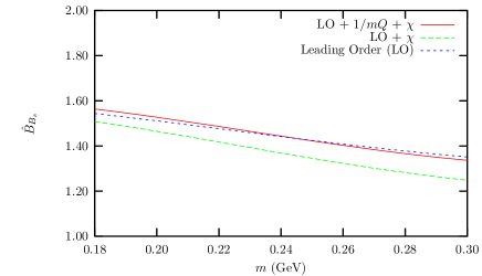
Figure 5: The bag parameter $\hat{B}$ for $B_{s}$ as a function of $m$.

5 The processes $B\rightarrow D\overline{D}$

For these processes there are only two relevant four quark operators. Within Heavy Quark Effective Theory (HQEFT) [9], the effective weak non-leptonic Lagrangian can be evolved down to the scale $\mu\sim\Lambda_{\chi}\sim$1 GeV [25]. The $b$, $c$, and $\overline{c}$ quarks are then treated within HQEFT.

Figure 6: Factorized contribution for $\overline{B^{0}}\rightarrow D^{+}D_{s}^{-}$ through the spectator mechanism, which does not exist for the decay mode $\overline{B^{0}}\rightarrow D_{s}^{+}D_{s}^{-}$ we consider in this paper. The double dashed lines represent heavy mesons, the double lines represent heavy quarks, and the single lines light quarks.

As an example of a typical factorized amplitude we choose the case $\overline{B^{0}}\rightarrow D^{+}D_{s}^{-}$ which is visualized in figure 6:

$$A(\overline{B^{0}}\rightarrow D^{+}D_{s}^{-})_{F}=$$ (38)

$$- \frac{G_{F}}{{\sqrt{2}}}V_{cb}V_{cs}^{*}\,a_{2}\,\zeta(\omega)f_{D}M_{D}\sqrt{M_{B}M_{D}}\;(\lambda+\omega)\;\,,$$

where $\zeta(\omega)$ is the Isgur-Wise function for the $\bar{B}\rightarrow D$ transition. Here $\omega\equiv v\cdot v^{\prime}=v\cdot\bar{v}=M_{B}/(2M_{D})$ and $\lambda\equiv\bar{v}\cdot v^{\prime}=(M_{B}^{2}/(2M_{D}^{2})-1)$, where $v$, $v^{\prime}$ and $\bar{v}$ are the velocities of the heavy $b$- $c$- and $\bar{c}$- quarks respectively. The Wilson coefficients $a_{i}$ contain short distance effects. Numerically, $a_{1}\sim 10^{-1}$ and $a_{2}\sim 1$ at the scale $\mu=m_{b}$. For $\mu<m_{c}$ the $a_{i}$’s are complex and one has $|a_{1}|\simeq 0.4$ and $|a_{2}|\simeq 1.4$ at $\mu\sim\Lambda_{\chi}\sim$1 GeV [25].

The factorized amplitude for $\overline{B^{0}}\rightarrow D_{s}^{+}D_{s}^{-}$ is visualized in figure 7. Unless one or both of the $D$-mesons in the final state are vector mesons, this matrix element is zero due to current conservation, which is analogous to the decay mode $\overline{D^{0}}\rightarrow K^{0}\overline{K^{0}}$ [6].

Figure 7: Factorized contribution for $\overline{B^{0}}\rightarrow D_{s}^{+}D_{s}^{-}$ through the annihilation mechanism, which give zero contributions if both $D_{s}^{+}$ and $D_{s}^{-}$ are pseudo-scalars.

In the following we will consider explicitly the decay mode $\overline{B^{0}}\rightarrow D_{s}^{+}D_{s}^{-}$. The analysis of $\overline{B^{0}_{s}}\rightarrow D^{+}D^{-}$ proceed the same way. To calculate the chiral loop amplitudes we need the factorized amplitudes for $\overline{B_{s}^{*0}}\rightarrow D_{s}^{+}D^{*-}$ and $\overline{B^{0}}\rightarrow D^{*+}D^{*-}$, which proceed through the spectator mechanism as in figure 6.

Figure 8: Non-factorizable chiral loops for $\overline{B^{0}}\rightarrow D_{s}^{+}D_{s}^{-}$.

We obtain the following chiral loop amplitude for the process $\overline{B^{0}}\rightarrow D_{s}^{+}D_{s}^{-}$ from the figure 8:

$$A(\overline{B^{0}}\rightarrow D_{s}^{+}D_{s}^{-})_{\chi}\,=\,\left(V_{cd}^{*}/V_{cs}^{*}\right)\,A(\overline{B_{d}^{0}}\rightarrow D_{d}^{+}D_{s}^{-})_{F}\cdot\;R^{\chi}\;\,,$$ (39)

where the factorized amplitude for the process $\overline{B^{0}}\rightarrow D^{+}D_{s}^{-}$ is given in (38).

The quantity $R^{\chi}$ is a sum of contributions from the left and right part of figure 8, and proportional to $(m_{K}{g_{{\cal A}}}/4\pi f)^{2}$ which is $1/N_{c}$ suppressed. Numerically,

$$R^{\chi}\;\simeq\;0.12-0.26i\;.$$ (40)

The genuine non-factorizable part for $\overline{B^{0}}\rightarrow D_{s}^{+}D_{s}^{-}$ at quark level can, by means of Fierz transformations and the identity (31), be written in terms of coloured currents.

The left part in figure 7 with gluon emission gives us the bosonized coloured current which is the same as for $B-\overline{B}$ mixing in eq. (33).

Figure 9: Non-factorizable contribution for $\overline{B^{0}}\rightarrow D_{s}^{+}D_{s}^{-}$ through the annihilation mechanism with additional soft gluon emission. The wavy lines represent soft gluons ending in vacuum to make gluon condensates.

For the creation of a $D\bar{D}$ pair in the right part of figure 7, there is an analogue of (33). We find the gluon condensate contribution for $\overline{B^{0}}\rightarrow D_{s}^{+}D_{s}^{-}$ within our model:

$$A(\overline{B^{0}}\rightarrow D_{s}^{+}D_{s}^{-})_{G}\;=$$ (41)

$$- \frac{G_{F}}{\sqrt{2}}V_{cb}V_{cq}^{*}\,a_{2}\,{\langle}\frac{\alpha_{s}}{\pi}G^{2}{\rangle}\;\frac{(G_{H}\sqrt{M_{B}})^{3}}{384m}\,F_{G}\;\;,$$

where $F_{G}$ is a dimensionless complex function of $\lambda$. The ratio between this amplitude and the factorized one in (38) scales as $M_{D}/(N_{c}M_{B})$ times hadronic parameters calculated within HL$\chi$QM. We define a quantity $R^{G}$ for the gluon condensate amplitude (41) analogously to $R^{\chi}$ in (39) for chiral loops. Numerically, we find that the ratio between the two amplitudes in (41) and (38) is

$$R_{G}\;\simeq\;0.055+0.16i\;\;,$$ (42)

which is of order one third of the chiral loop contribution in eq. (40).

Note that our non-factorizable amplitudes in (39) and (41) are proportional to the numerically favourable Wilson coefficient $a_{2}$.

We find the branching ratios

$$BR(\overline{B^{0}_{d}}\to D_{s}^{+}D_{s}^{-})\simeq 7\times 10^{-5}\;\;,$$ (43)

$$\quad BR(\overline{B^{0}_{s}}\to D^{+}D^{-})\simeq 1\times 10^{-3}\;\;.$$ (44)

The difference between the two branching ratios is mainly due to the difference in KM factor. For further details we refer to [4].

As mentioned above, the decay mode $\overline{D^{0}}\rightarrow K^{0}\overline{K^{0}}$ [6] is analogues to $\overline{B^{0}_{d}}\to D_{s}^{+}D_{s}^{-}$ in the sense that there are only non-factorizable contributions. The soft gluonic effects are similar to that in figure 9, but with $b$ replaced by $c$, which means that the left part of the diagram can still be described within HL$\chi$QM. In the right part of the diagram, $c\bar{c}$ has to be replaced by $s\bar{s}$, and $s$ replaced by $d$. In addition there is a mass insertion for the light quark part. However, the chiral loop diagrams are rather different in the two cases because there is only light mesons in the final state for the mode $\overline{D^{0}}\rightarrow K^{0}\overline{K^{0}}$.

6 The process $B\rightarrow D\,\eta^{\prime}$

Within the HL$\chi$QM, gluonic aspects of $\eta^{\prime}$ may be treated [5]. Using Fierz transformations for the four quark operators for $b\rightarrow cd\bar{u}$, we obtain contributions corresponding to figure 10.

Figure 10: Gluon condensate contributions to $B\rightarrow D\eta^{\prime}$.

In our approach two gluons are emitted from the light quark lines. One of these (the virtual $g^{*}$) attach to the $\eta^{\prime}gg^{*}$-vertex, and the other end in vacuum and make a gluon condensate together with one of the other soft gluons ($g$) from the $\eta^{\prime}gg^{*}$-vertex. This vertex which can be written:

$$-\frac{1}{2}F_{\eta^{{}^{\prime}}g^{*}g}\delta^{ab}\varepsilon^{\mu\nu\rho\sigma}\varepsilon_{\mu}^{*a}G_{\nu\rho}^{b}(0)\,q_{\sigma}\;\,$$ (45)

where $G(0)$ is the soft gluon tensor, $\varepsilon$ is the polarization vector of the virtual gluon, and $q$ is the momentum of the $\eta^{\prime}$. We have used existing parameterizations of the $\eta^{\prime}gg^{*}$-vertex form factor $F$ in (45) from the literature (at a scale of order 1 GeV they are numerically not very different). We have assumed that the current for $B\rightarrow g^{*}$ is related to the better known case $B\rightarrow\rho$:

$$J^{\mu a}(B\rightarrow g^{*d})= {\langle}g^{*d}|\overline{b}t^{a}\gamma^{\mu}(1-\gamma_{5})d|B{\rangle}$$

$$= \frac{\delta^{ad}}{2}\frac{g_{s}f_{\rho}}{m_{\rho}^{2}}{\langle}\rho|\overline{b}\gamma^{\mu}(1-\gamma_{5})d|B{\rangle}$$

It turns out that the “factorizable” diagram to the left in figure 10 can be neglected compared to the non-factorizable diagram to the right. Using the knowledge of the $B\rightarrow\rho$ current matrix element, we obtain the result [5]

$$Br(B\rightarrow D\eta^{{}^{\prime}})\,=\,(2.2\,\pm\,0.4)\,\times\,10^{-4}\;\,,$$ (46)

for $m$ in the range 230-270 MeV.

7 The $\beta$ term for $D^{*}\to D\gamma$

The chiral Lagrangian $\beta$-term has the form [19, 26]:

$${\cal L}_{\beta}=\frac{e\beta}{4}Tr[\overline{H}\,H\,\sigma\cdot F\,Q_{q}^{\xi}]\,.$$ (47)

Here $Q^{\xi}_{q}=(\xi^{\dagger}Q_{q}\xi+\xi Q_{q}\xi^{\dagger})/2$, where $Q_{q}$ is the $SU(3)$ charge matrix for light quarks, $Q_{q}=diag(-2/3,-1/3,-1/3)$, and $F$ is the electromagnetic field tensor. The $\beta$ term can be calculated in HL$\chi$QM, by considering diagrams which look like those in figure 1, but with the vector and axial vector fields ${\cal V}_{\mu}$ or ${\cal A}_{\mu}$ replaced by a photon field tensor. To leading order, we obtained the following expression :

$$\beta_{LO}=\frac{G_{H}^{2}f^{2}}{2m^{2}}\left\{1+\frac{N_{c}m^{2}}{4\pi f^{2}}-\left(\frac{56+3\pi}{576f^{2}m^{2}}\right){\langle}\frac{\alpha_{s}}{\pi}G^{2}{\rangle}\right\}\,.$$ (48)

As seen from figure 11, $\beta$ depends strongly on the constituent light quark mass $m$ because there is a partial cancellation between large terms in (48).

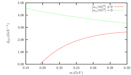
Figure 11: $\beta_{LO}$ as a function of the constituent light quark mass with and without gluon condensate.

One may hope that $1/m_{c}$ corrections might help to stabilize the result , but this is not the case. In fact, $1/m_{c}$ corrections do not play a significant role for $m>$ 230 MeV. (For smaller $m$ they even pull in the wrong direction compared to the experimental value of order 2-3 GeV^-1 [7]). To obtain a value close to the experimental value for $\beta$, we need a value for $m$ higher than used in [3, 8]. Choosing $m$ in the range 250-300 MeV we find $\beta=(2.5\pm 0.6)$ GeV^-1 to be compared with $\beta=(2.7\pm 0.20)$ GeV^-1 extracted from experiment. For further details we refer to [7].

8 Conclusion

In [8] we have constructed a heavy-light chiral quark model including soft gluonic effects and chiral loops. The model describes the heavy-light sector reasonably well[3, 4, 5, 6, 7, 8]. There is, however a difference compared to the pure light sector where $f_{\pi}$ is precisely known. If $f_{D}$ and $f_{B}$ had been more precisely known, we would have used them as numerical input (together with ${g_{{\cal A}}}$) to fix $m$ and ${\langle}\,\overline{q}q\,{\rangle}$ within the model. Instead we have used typical values of $m$ and ${\langle}\,\overline{q}q\,{\rangle}$ (and ${g_{{\cal A}}}$) as input, while $f_{D}$ and $f_{B}$ become output. (For a very recent review on numerical values for $f_{D}$ and $f_{B}$, see [27])

The value of $\beta$ turned out to be rather unstable [7] for the values of $m$ and ${\langle}\,\overline{q}q\,{\rangle}$ used in [3, 8]. Higher values of $m$ are needed to obtain an acceptable $\beta$ in agreement with experiment. However, this will lead to values of $f_{B}$ and $f_{D}$ which are too small . This can be compensated by using a higher value of the quark condensate ${\langle}\,\overline{q}q\,{\rangle}$. This is acceptable because our model dependent quantities ${\langle}\,\overline{q}q\,{\rangle}$ and ${\langle}\frac{\alpha_{s}}{\pi}G^{2}{\rangle}$ are not necessarily exactly those obtained in QCD sum rules.

Table 1: Numerical values for the $B$-sector.

	Input values I	Input values II
$G_{H}$	$\quad(8.3\pm 0.7)\,$ GeV-1/2	$\quad(7.2\pm 0.5)\,$ GeV-1/2
${\langle}\frac{\alpha_{s}}{\pi}G^{2}{\rangle}^{1/4}$	$\quad(300\pm 25)\,$ MeV	$\quad(340\pm 20)\,$ MeV
$f_{B}$	$\quad(190\pm 50)\,$ MeV	$\quad(185\pm 30)\,$ MeV
$f_{B_{s}}$	$\quad(210\pm 70)\,$ MeV	$\quad(215\pm 45)\,$ MeV
$f_{B_{s}}/f_{B}$	$\quad 1.14\pm 0.07$	$\quad 1.22\pm 0.02$
$\hat{B}_{B_{d}}$	$\quad 1.51\pm 0.09$	$\quad 1.52\pm 0.07$
$\hat{B}_{B_{s}}$	$\quad 1.4\pm 0.1$	$\quad 1.4\pm 0.1$
$\xi$	$\quad 1.08\pm 0.07$	$\quad 1.16\pm 0.04$

In Table 1 we have given our numerical values for a few important quantities in the $B$-sector. We have considered two sets of input. The first one is I: $m$ = 190 to 250 MeV and $-{\langle}\,\overline{q}q\,{\rangle}^{1/3}$ = 230 to 250 MeV [3, 7]. The second one is II: $m$ = 250 to 300 MeV and $-{\langle}\,\overline{q}q\,{\rangle}^{1/3}$ = 250 to 270 MeV [7]. In both cases, ${g_{{\cal A}}}=0.59$. For further details we refer to [3, 7, 8]. Note that the quantity $\xi$ in the table is defined as $\xi=\left(f_{B_{s}}\sqrt{\hat{B}_{B_{s}}}\right)/\left(f_{B_{d}}\sqrt{\hat{B}_{B_{d}}}\right)$ as usual. We observe that $\hat{B}$ is very stable with respect to variations in the input parameters.

Our model [8] is different from [15, 16] in the sense that we include the (phenomenological) gluon condensate. The figures 11 and 12 illustrates the importance of the gluon condensate at different values of $m$. In figure 12 the curves will be lifted for the quark condensate value II.

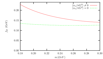
Figure 12: $f_{B}$ as a function of the constituent light quark mass with and without gluon condensate.

References

-
[1]
M. Beneke, G. Buchalla, M. Neubert, C.T. Sachrajda,
Phys. Rev. Lett. 83 (1999) 1914. - [2] C. Sachrajda, talk at this conference.
- [3] A. Hiorth and J.O. Eeg, Eur. Phys. J. direct C 30 (2003) 006.)
- [4] Jan.O. Eeg, Svjetlana Fajfer, and Aksel Hiorth, Phys. Lett. B 570 (2003) 46-52). J.O. Eeg, S. Fajfer, and A. Hiorth. Contributed to 21st International Symposium on Lepton and Photon Interactions at High Energies (LP 03), Batavia, Illinois, 11-16 Aug 2003. hep-ph/0307042.
- [5] J. O. Eeg, A. Hiorth, A. D. Polosa, Phys. Rev. D 65 (2002) 054030.
- [6] J. O. Eeg, S. Fajfer, and J. Zupan, Phys. Rev. D 64 (2001) 034010.
- [7] A. Hiorth and J.O. Eeg, hep-ph/0304247
- [8] A. Hiorth and J. O. Eeg, Phys. Rev. D66 (2002) 074001.
- [9] See for example A.V. Manohar, M.B. Wise, in “Heavy Quark Physics”, published in Cambridge Monogr. Part. Phys. Nucl. Phys. Cosmol. 10 (2000). M. Neubert, Phys. Rep. 245 (1994) 259.
- [10] B. Grinstein and A. Falk, Phys. Lett B 247 (1990) 406.
- [11] D. Espriu, E. de Rafael and J. Taron, Nucl. Phys. B345 (1990) 22. A. Pich and E. de Rafael, Nucl. Phys. B358 (1991) 311. D. Ebert and M .K . Volkov, Phys.Lett. B 272 (1991), 86.
- [12] J. O. Eeg and I. Picek, Phys. Lett. B301 (1993) 423, and B323 (1994) 193. A.E. Bergan and J.O. Eeg, Phys. Lett. B 390 (1997) 420.
- [13] S. Bertolini, J.O. Eeg and M. Fabbrichesi, Nucl. Phys. B449 (1995) 197. V. Antonelli, S. Bertolini, J.O. Eeg, M. Fabbrichesi and E.I. Lashin, Nucl. Phys. B469 (1996) 143. S. Bertolini, J.O. Eeg, M. Fabbrichesi and E.I. Lashin, Nucl. Phys. B514 (1998) 93.
- [14] S. Bertolini, J.O. Eeg, M. Fabbrichesi and E.I. Lashin, Nucl. Phys. B514 (1998) 63.
- [15] W.A. Bardeen and C.T. Hill, Phys. Rev. D49 (1994) 409 .
- [16] M.A. Nowak, M. Rho, and I. Zahed, Phys.Rev. D48 (1993) 4370. D. Ebert, T. Feldmann R. Friedrich and H. Reinhardt, Nucl. Phys. B434 (1995) 619. A. Deandrea, N. Di Bartelomeo, R. Gatto, G. Nardulli, and A.D. Polosa, Phys. Rev. D58 (1998) 034004. A. Polosa, Riv. Nuovo Cimento 23 (11) (2000) 1. D. Ebert, T. Feldmann and H. Reinhardt, Phys.Lett. B388 (1996) 154.
-
[17]
V. Novikov, M. Shifman, A. Vainshtein, V. Zakharov,
Fortschr. Phys. 32 (1984) 11. - [18] W.A. Bardeen, E.J. Eichten, C.T. Hill, hep-ph/0305049. M.A. Nowak, M. Rho, I. Zahed, hep-ph/0307102. M. Suzuki, hep-ph/0307118.
-
[19]
R. Casalbuoni, A. Deandrea, N. Di Bartelomeo,
R. Gatto, F. Feruglio and G. Nardulli,
Phys. Rep. 281 (1997) 145. - [20] See for example: G. Buchalla, A. Buras, and M. Lautenbacher, Rev. Mod. Phys. 68 (1996) 1125.
- [21] J.M. Flynn, C.T. Sachrajda, Adv.Ser.Direct.High Energy Phys. 15 (1998) 402-452. D. Bećirević, D. Meloni, A. Retico, V. Gimenez , L. Giusti, V. Lubicz, G. Martinelli, Nucl. Phys. B 618 (2001) 241-258. L. Lellouch, Plenary talk at 31st International Conference on High Energy Physics (ICHEP 2002), Amsterdam, The Netherlands, 24-31 Jul 2002, hep-ph/0211359. D. Bećirević, P. Boucaud, V. Gimenez, C.J.D. Lin, V. Lubicz, G. Martinelli, M. Papinutto, C.T. Sachrajda, Presented at 20th International Symposium on Lattice Field Theory (LATTICE 2002), Boston, Massachusetts, 24-29 Jun 2002, hep-lat/0209131.
- [22] D. Melikhov and N. Nikitin, Phys. Lett. B 494 (2000) 229-236.
- [23] V. Giménez, Nucl. Phys. B 401 (1993) 116. M. Ciuchini, E. Franco, and V. Giménez, Phys.Lett. B 388 (1996) 167.
- [24] W. Kilian and T. Mannel Phys.Lett. B301 (1993) 382.
- [25] B. Grinstein, W. Kilian, T. Mannel, and M.B. Wise, Nucl. Phys. B 363 (1991) 19. R. Fleischer, Nucl. Phys. B 412 (1994) 201.
- [26] I.W. Stewart, Nucl. Phys. B529 (1998) 62.
- [27] D. Bećirević, Workshop on the CKM Unitary Triangle, IPPP Durham, April 2003, hep-ph/0310072.