READING THE NUMBER OF EXTRA DIMENSIONS IN THE SPECTRUM OF HAWKING RADIATION

Abstract

After a brief review of the production and decay of Schwarzschild-like $(4+n)$-dimensional black holes in the framework of theories with Large Extra Dimensions, we proceed to derive the greybody factors and emission rates for scalars, fermions and gauge bosons on the brane. We present and discuss analytic and numerical methods for obtaining the above results, and demonstrate that both the amount and type of Hawking radiation emitted by the black hole can help us to determine the number of spacelike dimensions that exist in nature.

1 Introduction

The idea of the existence of extra spacelike dimensions in nature has been revived during the last few years in an attempt to explain the gap between different energy scales [1]. It demands the introduction of (at least) one 3-brane, which plays the role of our 4-dimensional world on which all Standard Model fields are localized; on the other hand, gravity can propagate both on the brane and in the bulk – the spacetime transverse to the brane. The introduction of extra spacelike dimensions inevitably affects both gravitational interactions and particle physics phenomenology and may lead to modifications in standard cosmology [2]. In this talk, we will focus on the scenario that postulates the existence of Large Extra Dimensions [3], according to which, in nature, there are $n\geq 2$ extra, spacelike, compact dimensions with size $R\leq 1$ mm leading to

$$M_{P}^{2}\sim M_{*}^{2+n}\,R^{n}\,.$$ (1)

From the above, it becomes clear that if $R\gg l_{P}$, then the $(4+n)$-dimensional Planck mass, $M_{*}$, will be much lower than the 4-dimensional one, $M_{P}$.

The above scenario can easily accommodate the notion of the existence of Black Holes in the universe. These objects may appear in nature with a variety of sizes, therefore, a black hole with $l_{P}<r_{H}<R$ is clearly a higher-dimensional object that can be still treated semi-clasically. These mini black holes are centered on the brane because the ordinary matter that undergoes gravitational collapse is restricted to live on the brane. Such mini black holes may have been created in the early universe due to density perturbations and phase transitions. Recently, there was a novel proposal according to which small, higher-dimensional black holes may be created during scattering of highly energetic particles at colliders or at the earth’s atmosphere [4, 5, 6]. This may happen when any two partons of the colliding particles pass within the horizon radius corresponding to their centre-of-mass energy [7]. The created black holes will go through a number of stages in their life [5], namely: (i) the balding phase, where the black hole sheds the hair inherited from the original particles, and the asymmetry due to the violent production process (15% of the total energy); (ii) the spin-down phase, in which the black hole looses its angular momentum through the emission of Hawking radiation [8] and, possibly, through superradiance (25% of the total energy); (iii) the Schwarzschild phase, where the emission of Hawking radiation results in the decrease of its mass (60% of the total energy); and, (iv) the Planck phase, that starts when $M_{BH}\sim M_{*}$ and whose study demands a theory of quantum gravity.

In this work, we concentrate on the spherically-symmetric Schwarzschild phase of a $(4+n)$-dimensional black hole, which is the longer one and accounts for the greatest proportion of the mass loss through the emission of Hawking radiation. The spacetime around such a black hole is given by [9]

$$ds^{2}=-\left[1-\left(\frac{r_{H}}{r}\right)^{n+1}\right]\,dt^{2}+\left[1-\left(\frac{r_{H}}{r}\right)^{n+1}\right]^{-1}\,dr^{2}+r^{2}d\Omega_{2+n}^{2}\,,$$ (2)

where

$$d\Omega_{2+n}^{2}=d\theta^{2}_{n+1}+\sin^{2}\theta_{n+1}\,\biggl{(}d\theta_{n}^{2}+\sin^{2}\theta_{n}\,\Bigl{(}\,...+\sin^{2}\theta_{2}\,(d\theta_{1}^{2}+\sin^{2}\theta_{1}\,d\varphi^{2})\,...\,\Bigr{)}\biggr{)}\,.$$ (3)

In the above, $0<\varphi<2\pi$ and $0<\theta_{i}<\pi$, for $i=1,...,n+1$. The horizon radius and temperature of such a black hole are given by

$$r_{H}=\frac{1}{\sqrt{\pi}M_{*}}\left(\frac{M_{BH}}{M_{*}}\right)^{\frac{1}{n+1}}\left(\frac{8\Gamma\left(\frac{n+3}{2}\right)}{n+2}\right)^{\frac{1}{n+1}}\,,\quad T_{BH}={(1+n)\over 4\pi\,r_{H}}\,,$$ (4)

respectively, where $M_{BH}$ is the mass of the black hole.

A black hole with temperature $T_{BH}$ emits Hawking radiation  with an almost blackbody spectrum and an energy emission rate given by

$$\frac{dE(\omega)}{dt}=\sum_{j}{\sigma_{j}(\omega)\,\,\omega\over\exp\left(\omega/T_{BH}\right)\mp 1}\,\,\frac{d^{n+3}k}{(2\pi)^{n+3}}\,.$$ (5)

In the above, $\omega$ is the energy of the emitted particle, and the statistics factor in the denominator is $-1$ for bosons and $+1$ for fermions. The $\omega$-dependent factor $\sigma_{j}$, with $j$ being the total angular momentum number, is the so-called greybody factor that distorts the blackbody spectrum; this is due to the fact that any particle emitted by the black hole has to traverse a strong gravitational background before reaching the observer, and $\sigma_{j}$ stands for the corresponding transmission cross-section. If, for example, a scalar field of the form $\phi\,(t,r,\theta_{i},\varphi)=e^{-i\omega t}\,R_{\omega j}(r)\,{Y}_{j}(\Omega)$ propagates in the background of Eq. (2), its radial equation of motion, in terms of the ‘tortoise’ coordinate $y=\frac{\ln h(r)}{r_{H}^{n+1}\,(n+1)}$, with $h(r)=1-(\frac{r_{H}}{r})^{n+1}$, reads

$$\left(-\frac{d^{2}\,}{dy^{2}}+r^{2n+4}\left[-\omega^{2}+\frac{j(j+n+1)h(r)}{r^{2}}\right]\right)R(y)=0\,.$$ (6)

The quantity inside square brackets gives the potential barrier in the $r>r_{H}$ area, and its expression reveals the fact that all parameters $(\omega,j,n)$ affect the value of $\sigma_{j}$. The latter is formally defined as [10]

$$\sigma_{j}(\omega)=\frac{2^{n}\pi^{(n+1)/2}\,\Gamma[(n+1)/2]}{n!\,\omega^{n+2}}\,\frac{(2j+n+1)\,(j+n)!}{j!}\,|{\cal A}_{j}|^{2}\,,$$ (7)

where ${\cal A}_{j}$ is the corresponding Absorption Probability for a particle moving towards the black hole.

The $(4+n)$-dimensional black hole (2) emits Hawking radiation both in the bulk and on the brane. Under the assumptions of the theory, only gravitons, and possibly scalar fields, live in the bulk and therefore these are the only particles that can be emitted in the bulk. On the other hand, the brane-localised modes include zero-mode scalars, fermions, gauge bosons and zero-mode gravitons. It is therefore much more interesting, from the observational point of view, to study the emission of brane-localised modes. The 4-dimensional background in which these modes propagate is the projection of the line-element (2) onto the brane, which is realized by setting $\theta_{i}=\pi/2$, for $i>1$. Then, we obtain

$$ds^{2}_{4}=-\left[1-\left(\frac{r_{H}}{r}\right)^{n+1}\right]\,dt^{2}+\left[1-\left(\frac{r_{H}}{r}\right)^{n+1}\right]^{-1}\,dr^{2}+r^{2}\,(d\theta^{2}+\sin^{2}\theta\,d\varphi^{2})\,.$$ (8)

The emission of brane-localised modes is a 4-dimensional process and the corresponding greybody factor takes the simplified form

$$\sigma_{j}(\omega)=\frac{\pi}{\omega^{2}}\,(2j+1)\,|{\cal A}_{j}|^{2}\,.$$ (9)

Nevertheless, ${\cal A}_{j}$ does depend on the number $n$ of extra dimensions projected onto the brane, through the expression of the line-element (8), and this valuable piece of information will be evident in the computed radiation spectrum.

2 Hawking radiation from a Black Hole on a 4-dimensional brane

In these section, we will briefly discuss the emission of brane-localised scalars, fermions and gauge bosons (for more information, see Refs. [11, 12, 13]). We will present analytic and numerical methods for deriving the desired results, and comment on the dependence of the amount and type of particles emitted on the brane on the number of extra dimensions.

The derivation of a master equation [13] describing the motion of a particle with arbitrary spin $s$ in the projected background (8) is the starting point of our analysis. By using the factorization

$$\Psi_{s}=e^{-i\omega t}\,e^{im\varphi}\,R_{s}(r)\,S_{s,j}^{m}(\theta)\,,$$ (10)

where $Y_{s,j}^{m}=e^{im\varphi}\,S_{s,j}^{m}(\theta)$ are the spin-weighted spherical harmonics [14], and by employing the Newman-Penrose method, we obtain the radial equation

$$\frac{1}{\Delta^{s}}\frac{d}{dr}\left(\Delta^{s+1}\frac{dR_{s}}{dr}\right)+\left[\frac{\omega^{2}r^{2}}{h}+2i\omega sr-\frac{is\omega r^{2}h^{\prime}}{h}+s(\Delta^{\prime\prime}-2)-\lambda_{sj}\right]R_{s}(r)=0,$$ (11)

where $\Delta=hr^{2}$ and $\lambda_{sj}=j(j+1)-s(s+1)$.

The above equation needs to be solved over the whole radial domain. This can be done either analytically or numerically with different advantages in each case. The analytic treatment demands the use of an approximate method in which the above equation is solved at the near-horizon regime ($r\simeq r_{H}$) and far-field regime ($r\gg r_{H}$), and the corresponding solutions are matched at an intermediate zone. This method allows us to solve the radial equation for particles with arbitrary spin $s$ in a unified way. This was done in Ref. [12], where the transformed, and slightly simpler, equation

$$\Delta^{s}\frac{d}{dr}\left(\Delta^{1-s}\frac{dP_{s}}{dr}\right)+\left[\frac{\omega^{2}r^{2}}{h}+2i\omega sr-\frac{is\omega r^{2}h^{\prime}}{h}-\Lambda_{sj}\right]P_{s}(r)=0$$ (12)

was used, where now $\Lambda_{sj}=j(j+1)-s(s-1)$ and $P_{s}(r)=\Delta^{s}R_{s}(r)$. At the near-horizon regime, a change of variable $r\rightarrow h(r)$ brings the above differential equation to a hypergeometric form. Under the boundary condition that only incoming modes must exist close to the horizon, its general solution reduces to

$$P_{NH}(h)=A_{h}\,h^{\alpha}\,(1-h)^{\beta}\,F(a,b,c;h)\,,$$ (13)

where $a=\alpha+\beta+\frac{s+n\,(1-s)}{(n+1)}$, $b=\alpha+\beta$, and $c=1-s+2\alpha$, with

$$\alpha=-\frac{i\omega r_{H}}{n+1},\quad\beta=\frac{1}{2(n+1)}\,\biggl{[}\,1-2s-\sqrt{(1+2j)^{2}-4\omega^{2}r_{H}^{2}-8is\omega r_{H}}\,\,\biggr{]},$$ (14)

and $A_{h}$ an arbitrary constant. At the far-field regime, on the other hand, by setting $r\gg r_{H}$ in Eq. (12), we obtain a confluent hypergeometric equation with solution:

$$P_{FF}(r)=e^{-i\omega r}r^{j+s}\Bigl{[}B_{+}\,M(j-s+1,2j+2,2i\omega r)+B_{-}\,U(j-s+1,2j+2,2i\omega r)\Bigr{]}\,,$$ (15)

where $M$ and $U$ are the Kummer functions and $B_{\pm}$ arbitrary coefficients. We finally match the two asymptotic solutions: we first expand the NH solution in the limit $r\gg r_{H}$, and the FF solution in the limit $\omega r\ll 1$. Both solutions then take the form $P=C_{1}r^{j}+C_{2}\,r^{-(j+1)}$, and the matching of the corresponding coefficients determines the ratios $B_{\pm}/A_{h}$. These constant ratios are involved in the definition of the Absorption Probability ${\cal A}_{j}$, that is defined as:

$$|{\cal A}_{j}|^{2}=\frac{{\cal F}_{in}^{(h)}}{{\cal F}_{in}^{(\infty)}}\,,$$ (16)

in terms of the energy fluxes evaluated at infinity and the horizon. The ratios $B_{\pm}/A_{h}$ are given by complicated expressions [11, 12] that depend on $\omega$, $r_{H}$, $j$ and $n$, and their behaviour, as any of these parameters change, is difficult to infer.

A usual manipulation is to expand these complicated expressions in the limit $\omega r_{H}\ll 1$. Then, by keeping the dominant term in the power series, we obtain simple, elegant expressions for ${\cal A}_{j}$; for example, in the case of scalar fields, this takes the form [11]

$$|{\cal A}_{j}|^{2}=\frac{16\pi}{(n+1)^{2}}\,\biggl{(}\frac{\omega r_{H}}{2}\biggl{)}^{2j+2}\,\frac{\Gamma(\frac{j+1}{n+1})^{2}\,\Gamma(1+\frac{j}{n+1})^{2}}{\Gamma(\frac{1}{2}+j)^{2}\,\Gamma(1+\frac{2j+1}{n+1})^{2}}+...\,.$$ (17)

According to the above, $|{\cal A}_{j}|^{2}$, and subsequently the greybody factor, decreases as $j$ increases while it gets enhanced as $n$ increases. Similar expressions and results are obtained for the emission of fermions and gauge fields.

Before using the simplified expressions for the evaluation of the emission rates from the black hole, let us check their validity. These expressions have been derived in the low-energy limit and thus we expect them to break down at intermediate values of $\omega r_{H}$. But can we trust them even in the low-energy regime? The full analytic expressions [11, 12] (the ones derived before expanding in power series in $\omega r_{H}$) can provide the answer. Although more complicated, these analytic expressions can be easily plotted to reveal the behavior in question. A simple analysis shows that, in the case of scalar fields, the greybody factor indeed decreases with $j$ but it also decreases with $n$, the latter being in apparent contradiction with Eq. (17). A similar analysis for the case of fermions and gauge fields leads to a satisfactory agreement with the simplified analytic expressions. So, what went wrong with the scalar fields? The main contribution to the greybody factor for spin-0 fields comes from the dominant first partial wave ($j=0$) in Eq. (17), which is found to be independent of $n$. Any dependence on $n$ must be therefore read from the higher partial waves which indeed are enhanced as $n$ increases. However, it turns out that the next-to-leading order terms, denoted by “…” in Eq. (17), are of the same order as the higher partial waves and should also be taken into account. When this is done, we are finally led to a decrease with $n$. This does not happen for fields with $s={1\over 2},1$ where the lowest partial wave has a non-trivial dependence on $n$.

Going back to the full analytic expressions for the absorption probability, we may safely use them to derive the greybody factors and emission rates since they include all subdominant corrections and thus have an extended validity up to higher energies. As mentioned above, the greybody factor for scalar fields is found [12] to decrease with $n$, while the ones for fermions and gauge bosons are enhanced as $n$ increases, at least up to intermediate energies. While scalars and fermions have a non-vanishing greybody factor as $\omega r_{H}\rightarrow 0$, the one for the gauge bosons vanishes. By using Eq. (5) with $n=0$, we may then compute the emission rates for different particles on the brane [12]. Despite the different behaviour of the greybody factors for scalars, fermions and gauge bosons, the corresponding emission rates exhibit a universal behaviour according to which the energy emitted per unit time and energy interval is strongly enhanced as $n$ increases up to intermediate values of the energy parameter $\omega r_{H}$.

But what about the high-energy behaviour? The full analytic expressions for the absorption coefficient, although of extended validity compared to the simplified ones, are not valid in the high-energy regime. The assumption that $\omega r_{H}\ll 1$ was made in the matching process, therefore, these expressions are also bound to break down at some point. The only way to derive exact results valid at all energy regimes is through numerical integration. This task was performed in Ref. [13] where both greybody factors and emission rates were computed. The exact results for the greybody factors closely follow the ones predicted by the full analytic results at the low- and intermediate-energy regimes. At the high-energy regime, a universal asymptotic behaviour, the same for all particle species, is revealed: the black hole acts as an absorptive area of radius [15] $r_{c}$ that leads to a blackbody spectrum with $\sigma\simeq\pi r_{c}^{2}$. The effective radius $r_{c}$ is $n$-dependent and decreases as the value of $n$ increases [16].

The energy emission rates determined by the numerical analysis also agree with the ones derived by using the full analytic expressions up to intermediate energies. Whereas the analytic results covered only a part of the “greybody” curve, especially as the spin of the particle and the number of extra dimensions increased, the numerical results allow us to derive the complete radiation spectrum. In Fig.1, we depict the energy emission rates for fermions on the brane. The enhancement of the rate, at which energy is radiated on the brane, as $n$ increases, is indeed impressive reaching orders of magnitude for large values of $n$, and for all species of particles. This is mainly due to the increase in the temperature of the black hole that automatically increases the amount of energy that can be spent on the emission of particle modes. Apart from the increase in the height and width of each curve, a Wien’s type of displacement of the peak towards higher energies also takes place.

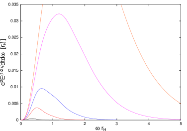
Figure 1: Energy emission rates for fermions on the brane by a Schwarzschild-like (4+n)D black hole. The lines correspond to $n=0,1,2,4$ and 6, respectively, increasing upwards.

The magnitude of the enhancement of the emission rates is different for different species of particles. This evidently changes the type of particle that the black hole prefers to emit, as the number of extra dimensions changes. In 4 dimensions [17, 18], most of the energy of the black hole is spent on the emission of scalar degrees of freedom, with the emission of fermions and gauge degrees [19] being subdominant. Our analysis [13] reveals that the latter two species take only 0.55 and 0.23, respectively, of the energy spent on the scalar “channel”. As $n$ increases, however, these numbers drastically change: for $n=2$, the relative emissivities become 1 : 0.91 : 0.91, and, for $n=6$, 1 : 0.84 : 1.06. Therefore, for intermediate values of $n$, the black hole spends the same amount of energy for the emission of fermions and gauge bosons, while, for large values of $n$, the emission of gauge fields is the dominant “channel”.

In conclusion, the detection of Hawking radiation from a decaying black hole is an exciting challenge on its own. If Extra Dimensions exist, the emission spectra can also help us to determine the dimensionality of spacetime, even if we look only at the energy emitted on the brane (for exact results on the Bulk-to-Brane relative emissivities, see [13]). Distinctive features of the $n$-dependent spectrum is the amount and type of radiation emitted by the black hole, and the improvement of the spectrum by implementing the exact greybody factors is imperative in order to accomplish this task in an accurate way.

References

References

- [1] I. Antoniadis, Phys. Lett. B 246, 377 (1990); P. Horava and E. Witten, Nucl. Phys. B 460, 506 (1996); J. D. Lykken, Phys. Rev. D 54, 3693 (1996); K. Dienes, E. Dudas and T. Gherghetta, Phys. Lett. B 436, 55 (1998); L. Randall and R. Sundrum, Phys. Rev. Lett. 83, 3370 (1999).
- [2] P. Kanti, I. I. Kogan, K. A. Olive and M. Pospelov, Phys. Lett. B 468, 31 (1999); Phys. Rev. D 61, 106004 (2000).
- [3] N. Arkani-Hamed, S. Dimopoulos and G. Dvali, Phys. Lett. B 429, 263 (1998); Phys. Rev. D 59, 086004 (1999); I. Antoniadis, N. Arkani-Hamed, S. Dimopoulos and G. R. Dvali, Phys. Lett. B 436, 257 (1998).
- [4] T. Banks and W. Fischler, hep-th/9906038.
- [5] S. B. Giddings and S. Thomas, Phys. Rev. D65, 056010 (2002).
- [6] S. Dimopoulos and G. Landsberg, Phys. Rev. Lett. 87, 161602 (2001).
- [7] K. S. Thorne, in Magic without Magic, Ed. J. R. Klauder (1972).
- [8] S. W. Hawking, Comm. Math. Phys. 43, 199 (1975).
- [9] R. C. Myers and M. J. Perry, Ann. Phys. (NY) 172, 304 (1986).
- [10] S. Gubser, I. Klebanov and A. Tseytlin, Nucl. Phys. B499, 217 (1997).
- [11] P. Kanti and J. March-Russell, Phys. Rev. D66, 024023 (2002).
- [12] P. Kanti and J. March-Russell, Phys. Rev. D67, 104019 (2003).
- [13] C. M. Harris and P. Kanti, J. High Energy Phys. 0310, 014 (2003).
- [14] J. N. Goldberg et al., J. Math. Phys. 8, 2155 (1967).
- [15] N. Sanchez, Phys. Rev. D18, 1030 (1978); ibid. D18, 1798 (1978).
- [16] R. Emparan, G. Horowitz and R. Myers, Phys. Rev. Lett. 85, 499 (2000).
- [17] D. N. Page, Phys. Rev. D13, 198 (1976).
- [18] J. H. MacGibbon and B. R. Webber, Phys. Rev. D41, 3052 (1990).
- [19] For the emission of elementary particles, see Ref. [6] and C. M. Harris, P. Richardson and B. R. Webber, J. High Energy Phys. 0308, 033 (2003).