DCPT /03/110

IPPP /03/55

MADPH 03-1348

hep-ph/0310156

QCD corrections to electroweak
$\ell\nu_{\ell}jj$ and $\ell^{+}\ell^{-}jj$ production

Carlo Oleari¹ and Dieter Zeppenfeld^{2 1} Department of Physics, University of Durham, South Road, Durham DH1 3LE, UK
² Department of Physics, University of Wisconsin, Madison, WI 53706, USA

The production of $W$ or $Z$ bosons in association with two jets is an important background to the Higgs boson search in vector-boson fusion at the LHC. The purely electroweak component of this background is dominated by vector-boson fusion, which exhibits kinematic distributions very similar to the Higgs boson signal. We consider the next-to-leading order QCD corrections to the electroweak production of $\ell\nu_{\ell}jj$ and $\ell^{+}\ell^{-}jj$ events at the LHC, within typical vector-boson fusion cuts. We show that the QCD corrections are modest, increasing the total cross sections by about 10%. Remaining scale uncertainties are below 2%. A fully-flexible next-to-leading order partonic Monte Carlo program allows to demonstrate these features for cross sections within typical vector-boson-fusion acceptance cuts. Modest corrections are also found for distributions.

1 Introduction

Vector-boson fusion (VBF) processes have emerged as a particularly interesting class of scattering events from which one hopes to gain insight into the dynamics of electroweak symmetry breaking. The most prominent example is Higgs boson production via VBF, that is, the process $qq\,\mbox{$\rightarrow$}\,qqH$, which can be viewed as quark scattering via $t$-channel exchange of a weak boson, with the Higgs boson radiated off the $W$ or $Z$ propagator. Alternatively, one may view this process as two weak bosons fusing to form the Higgs boson. The kinematic characteristics of this process are very distinctive: two jets, in the forward and backward region of rapidity, with the Higgs boson decay products in the central region of the detector. This characteristic signature greatly helps to distinguish these $Hjj$ events from backgrounds. Higgs boson production via VBF has been studied intensively as a tool for Higgs boson discovery [1, 2] and the measurement of Higgs boson couplings [3] in $pp$ collisions at the CERN Large Hadron Collider (LHC).

Analogous to Higgs boson production via VBF, the electroweak production of a $W$ or $Z$ plus two jets, with the requirement that the weak boson is centrally produced and that the two jets are well separated in rapidity, will proceed with sizable cross section at the LHC. The decay leptons in $W\,\mbox{$\rightarrow$}\,\ell\nu_{\ell}$ and $Z\,\mbox{$\rightarrow$}\,\ell^{+}\ell^{-}$ lead to the final states $\ell\nu_{\ell}jj$ and $\ell^{+}\ell^{-}jj$ ($\ell=e,\mu,\tau$). These processes have already been considered in the literature at leading order (LO). To name but a few examples, they have been studied in the investigation of rapidity gaps at hadron colliders [6, 7, 8], as a probe of anomalous triple-gauge-boson couplings [9] or as a background to Higgs boson searches in VBF [10, 11, 12]. In this last case, the $\ell\nu_{\ell}jj$ final state with an unidentified charged lepton, or $\nu_{\ell}\bar{\nu}_{\ell}jj$ events from $Z\mbox{$\rightarrow$}\nu_{\ell}\bar{\nu}_{\ell}$ decay, form a background to invisible Higgs boson decay (see e.g. Ref. [12]). $\tau^{+}\tau^{-}jj$ events are a background to the decay $H\,\mbox{$\rightarrow$}\,\tau^{+}\tau^{-}$ [10], and also to $H\,\mbox{$\rightarrow$}\,W^{+}W^{-}$ when the $W$’s and the $\tau$’s decay leptonically [11]. In these examples, off-shell corrections to $Z\,\mbox{$\rightarrow$}\,\tau^{+}\tau^{-}$ decay need to be included, since a Higgs boson mass in the range $114~{}{\rm GeV}<m_{H}<200~{}{\rm GeV}$, well above the $Z$ peak, is favored by electroweak data [13].

While a LO analysis is perfectly adequate for exploratory investigation, precision measurements at the LHC require comparison with cross-section predictions which include higher-order QCD corrections. A poignant example is the extraction of Higgs boson couplings, where expected accuracies of the order of 10%, or even better [3], clearly require knowledge of the next-to-leading order (NLO) QCD corrections. In addition, one would like to exploit $W$ and $Z$ production, in VBF configurations, as calibration processes for Higgs boson production via VBF, namely as a tool to understand the tagging of forward jets or the distribution and veto of additional central jets in VBF (see e.g. Ref. [7, 8]). In fact, these processes share the same color structure: two colored quarks are scattered via the exchange of a colorless boson in the $t$-channel. The pattern of soft gluon radiation is then the same. Understanding the gap-survival probability in the known case of $W$ and $Z$ production can give insight on the gap survival for the case of Higgs boson production. The precision needed for Higgs boson studies and for the understanding of radiation patterns then requires the knowledge of NLO QCD corrections for $Wjj$ and $Zjj$ production as well.

The NLO QCD corrections to the total $Hjj$ cross section from VBF has been known for many years [14]. In a recent paper [15], we presented the calculation of these corrections in the form of a fully-flexible parton-level Monte Carlo program which allows the determination of NLO corrections to arbitrary (infrared-safe) distributions. Here, we extend this work and describe the calculation and first results for such corrections to $Wjj$ and $Zjj$ production in VBF configurations. To be precise, since the decaying weak bosons are spin-one particles, in order to retain all the possible angular correlations between the final state particles, we consider the electroweak processes $pp\,\mbox{$\rightarrow$}\,\ell^{\pm}\nu_{\ell}jjX$ and $pp\,\mbox{$\rightarrow$}\,\ell^{+}\ell^{-}jjX$ at NLO.

Figure 1: Feynman graphs contributing to the process $uc\,\mbox{$\rightarrow$}\,dc\ell^{+}\nu_{\ell}$ at tree level. For the generic VBF process discussed in this paper, seven Feynman-graph topologies contribute at tree level: the six topologies shown plus an additional bremsstrahlung graph, with the vector boson emitted off the final-state charm quark [mirror image of graph (b)].

At LO, Feynman graphs for one such process, $uc\,\mbox{$\rightarrow$}\,dcW^{+},W^{+}\,\mbox{$\rightarrow$}\,\ell^{+}\nu_{\ell}$, are shown in Fig. 1. Using the terminology introduced in [16], we consider bremsstrahlung (a, b, c), fusion (d) and multiperipheral (e, f) diagrams. We neglect diagrams corresponding to conversion, abelian and non-abelian annihilation, since these $q\bar{q}$ annihilation contributions are negligible when we impose VBF cuts, as explained in detail in Sec. 2.1.

In the following, in order to use a shorthand notation, we will call processes such as the one depicted in Fig. 1 “EW $Vjj$ production”, or VBF production of $W/Z$ plus two jets, since we consider these processes with the kinematic cuts typical for the selection of VBF (see Sec. 4). It should be understood that, in spite of this notation, multiperipheral diagrams like (e) and (f) are included, even though they cannot be represented as the production of a weak boson, followed by its decay into two leptons.

The structure of the paper is as follows: in Sec. 2, we outline the calculation of the tree-level diagrams, of real-emission contributions and of the virtual corrections. We dedicate Sec. 2.3 to the discussion of the virtual contributions, with some of the analytical details relegated to Appendix A. A list of checks which we have performed on our calculation concludes Sec. 2. Additional features of our Monte Carlo program, like the gauge invariant handling of finite $W$ and $Z$ widths, the inclusion of anomalous $WW\gamma$ and $WWZ$ couplings, the approximations with regard to crossed diagrams in the presence of identical quark flavors, the singularities for incoming photons and the choice of parameters, will be discussed in Sec. 3. We then use this Monte Carlo program to present first results for EW $Vjj$ production at the LHC. Of particular concern is the scale dependence of the NLO results, which provides an estimate for the residual theoretical error of our cross-section calculations. We discuss the scale dependence and the size of the radiative corrections for various distributions in Sec. 4. Conclusions are given in Sec. 5.

2 Elements of the calculation

The structure of the three processes under consideration, $pp\,\mbox{$\rightarrow$}\,\ell^{+}\nu_{\ell}jjX$, $pp\,\mbox{$\rightarrow$}\,\ell^{-}\bar{\nu}_{\ell}jjX$ and $pp\,\mbox{$\rightarrow$}\,\ell^{+}\ell^{-}jjX$, is very similar. A discussion of any single one of them is sufficient to clarify our procedures for all, and we use $W^{+}$ production, i.e., the calculation of the $pp\,\mbox{$\rightarrow$}\,\ell^{+}\nu_{\ell}jjX$ cross section, for this purpose. Mutatis mutandis, all the considerations apply to the other processes too.

2.1 Approximations and general framework

At tree level, the topological structure of the generic subprocesses contributing to EW $Wjj$ production is depicted in Fig. 1. Two additional classes of diagrams appear in case of identical quark flavors on two of the fermion lines:

• diagrams where both the two virtual vector bosons are time-like. They correspond to diagrams called conversion, abelian and non-abelian annihilation in Ref. [16], and contain vector-boson pair production with subsequent decay of one of the weak bosons to a pair of jets. Pars pro toto, we call this class vector-boson pair production in the following.

• diagrams obtained by interchange of identical initial- or final-state (anti)quarks, such as in the $uu\,\mbox{$\rightarrow$}\,du\ell^{+}\nu_{\ell}$ or $du\,\mbox{$\rightarrow$}\,dd\ell^{+}\nu_{\ell}$ subprocesses.

These additional diagrams are obtained from the ones shown in Fig. 1 by crossing. In our calculation, we have neglected contributions from vector-boson pair production completely. In addition, any interference effects of the second class with the graphs of Fig. 1 are neglected. This is justified because, in the phase-space region where VBF can be observed experimentally, with widely-separated quark jets of very large invariant mass, the neglected terms are strongly suppressed by large momentum transfer in one or more weak-boson propagators. Color suppression further reduces any interference terms. We have checked with MadEvent [17] that, at LO, the diagrams that we have not considered and interference effects contribute less than 0.3% to our final results in e.g. Fig. 4. Since we expect QCD corrections to the neglected terms to be modest, the above approximations are fully justified within the accuracy of our NLO calculation.

Fermion masses are set to zero throughout, because observation of either leptons or (light) quarks in a hadron-collider environment requires large transverse momenta and hence sizable scattering angles and relativistic energies. For the $t$-channel processes which we include, we have used a diagonal form (equal to the identity matrix) for the Cabibbo-Kobayashi-Maskawa matrix, $V_{CKM}$. This approximation is not a limitation of our calculation. As long as no final-state quark flavor is tagged (no $c$ tagging is done, for example), the sum over all flavors, using the exact $V_{CKM}$, is equivalent to our results, due to the unitarity of the $V_{CKM}$ matrix.

2.2 Tree-level diagrams and real corrections

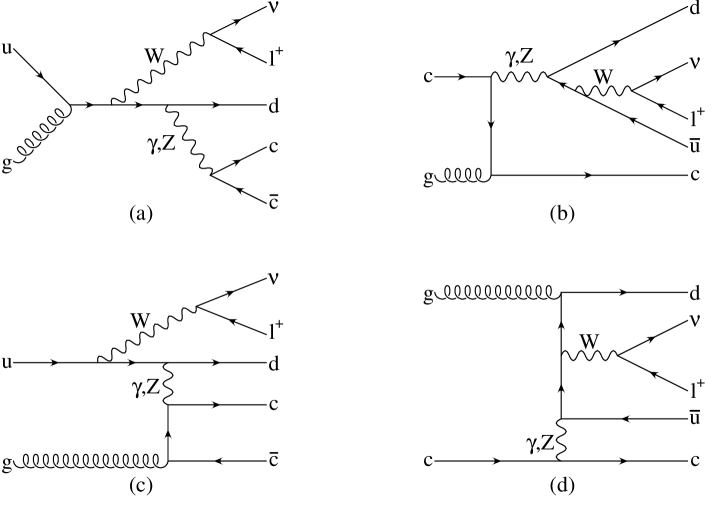
Figure 2: Examples of Feynman amplitudes with an initial gluon. Graphs like (a) and (b), with the gluon coupled to the initial quark line, correspond to vector-boson pair production and are eliminated. The two gauge-invariant subsets of graphs like (c) and (d), with the gluon coupled to the final-state quark pair, contain all $g\mbox{$\rightarrow$}q\bar{q}$ splitting contributions and are included in our calculation.

For the $Wjj$ Born amplitude, we need to add the contributions from the 10 Feynman graphs shown in Fig. 1 ($Z$ and $\gamma$ propagators counted as different diagrams), and sum cross sections of all subprocesses producing $W^{+}$ plus two jets. The same is true for $W^{-}$ production. For the case of $Zjj$ production, amplitudes which correspond to neutral-current exchange (no change of quark flavors) receive contributions from 24 Feynman graphs at tree level. To obtain the real-emission diagrams, with a final-state gluon, one needs to attach the gluon to the quark lines in all possible ways. For the diagrams in Fig. 1, this gives rise to 45 real-emission graphs. 112 different Feynman graphs contribute to real-emission corrections to $Zjj$ production via neutral-current exchange.

The contributions with an initial-state gluon are obtained by crossing the previous diagrams, promoting the final-state gluon as incoming parton, and an initial-state (anti)quark as final-state particle. We again remove all diagrams where two time-like, final-state vector bosons appear such as $gu\,\mbox{$\rightarrow$}\,\ell^{+}\nu_{\ell}dZ^{*}$, with $Z^{*}\,\mbox{$\rightarrow$}\,c\bar{c}$. Such diagrams, for consistency, must be removed since we have not considered the corresponding Born contributions. Figure 2 clarifies this issue: we drop all initial-gluon contributions in which the gluon couples to the fermion line of the initial quark or antiquark. In fact, these diagrams are strongly suppressed when VBF cuts (see Sec. 4) are applied to the final-state jets.

Our Monte Carlo program computes all amplitudes numerically, using the formalism of Ref. [18]. The Born amplitudes for $W$ and $Z$ production are taken from Ref. [6]. The real-emission amplitudes for $Z$ production were first given in Ref. [7]. The corresponding amplitudes for $W$ production were partially programed at the time. We have finalized and tested them for the present application.

2.3 Virtual corrections

At NLO, we have to deal with soft and collinear singularities in the virtual and real-emission contributions. Our calculation uses the subtraction method of Catani and Seymour [19] to cancel the soft and collinear divergences between virtual and real-emission diagrams. Since these divergences only depend on the color structure of the external partons, the subtraction terms encountered for EW $Vjj$ production are identical in form to those found for Higgs boson production in VBF. Thus, we can use the results described in Ref. [15] for the case at hand. The main difference is that the finite parts of the virtual corrections are more complicated than for $Hjj$ production (where only vertex corrections were present).

The QCD corrections to EW $Vjj$ production appear as two gauge-invariant subsets, corresponding to corrections to the upper and lower fermion lines in Fig. 1. Due to the color singlet nature of the exchanged electroweak bosons, any interference terms between subamplitudes with gluons attached to both the upper and the lower quark lines vanish identically at order $\alpha_{s}$. Hence, it is sufficient to consider radiative corrections to a single quark line only, which we here take as the upper one. Corrections to the lower fermion line are an exact copy.

In computing the virtual corrections, we have used the dimensional reduction scheme [20]: we have performed the Passarino-Veltman reduction of the tensor integrals in $d=4-2\epsilon$ dimensions, while the algebra of the Dirac gamma matrices, of the external momenta and of the polarization vectors has been performed in $d=4$ dimensions.

We split the virtual corrections into two classes: the virtual corrections along a quark line with only one weak boson attached and the virtual corrections along a quark line with two weak bosons attached.

I. The virtual NLO QCD contribution to any tree level Feynman subamplitude ${\cal M}_{B}^{(i)}$ which has a single electroweak boson $V$ (of momentum $q$) attached to the upper fermion line,

$$q(k_{1})\,\mbox{$\rightarrow$}\,q(k_{2})+V(q)\;,$$ (2.1)

appears in the form of a vertex correction, which is factorisable in terms of the original Born subamplitude

$${\cal M}_{V}^{(i)}={\cal M}_{B}^{(i)}\frac{\alpha_{s}(\mu_{R})}{4\pi}C_{F}\left(\frac{4\pi\mu_{R}^{2}}{Q^{2}}\right)^{\epsilon}\Gamma(1+\epsilon)\left[-\frac{2}{\epsilon^{2}}-\frac{3}{\epsilon}+c_{\rm virt}+{\cal O}\left(\epsilon\right)\right]\,.$$ (2.2)

Here $\mu_{R}$ is the renormalization scale, and the boson virtuality $Q^{2}=-(k_{1}-k_{2})^{2}=-q^{2}$ is the only relevant scale in the process, since the quarks are assumed to be massless, $k_{1}^{2}=k_{2}^{2}=0$. In dimensional reduction, the finite contribution is given by $c_{\rm virt}=\pi^{2}/3-7$ ($c_{\rm virt}=\pi^{2}/3-8$ in conventional dimensional regularization).

II. The second class of diagrams are the virtual QCD corrections to the Feynman graphs where two electroweak bosons $V_{1}$ and $V_{2}$ (of outgoing momenta $q_{1}$ and $q_{2}$) are attached to the same fermion line (see, for example, the upper quark line in Fig. 1 (a, b)). It suffices to consider one of the two possible permutations of $V_{1}$ and $V_{2}$, as depicted in Fig. 3. The kinematics is given by

$$q(k_{1})\,\mbox{$\rightarrow$}\,q(k_{2})+V_{1}(q_{1})+V_{2}(q_{2})\,,$$ (2.3)

where $k_{1}^{2}=k_{2}^{2}=0$ and momentum conservation reads $k_{1}=k_{2}+q_{1}+q_{2}$. In the following, it is convenient to use the Mandelstam variables for a $2\,\mbox{$\rightarrow$}\,2$ process which we take as $q\bar{q}\,\mbox{$\rightarrow$}\,V_{1}V_{2}$. We then define

$$s=(k_{1}-k_{2})^{2}=(q_{1}+q_{2})^{2}\;,\quad t=(k_{1}-q_{1})^{2}=(k_{2}+q_{2})^{2}\;,\quad u=(k_{1}-q_{2})^{2}=(k_{2}+q_{1})^{2}\;.$$ (2.4)

In order to use the same notation as in Eq. (2.2), we define $Q^{2}=2k_{1}\cdot k_{2}\equiv-s$.

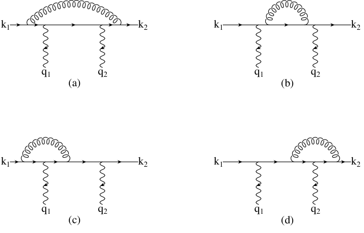
Figure 3: Virtual corrections for a fermion line with two attached electroweak bosons, $V_{1}(q_{1})$ and $V_{2}(q_{2})$. The finite part of the sum of these graphs defines the reduced amplitude $\tilde{\cal M}_{\tau}(q_{1},q_{2})$ of Eq. (2.5).

The two electroweak bosons are always virtual in our calculation, i.e., the effective polarization vectors $\epsilon_{1}(q_{1})$ and $\epsilon_{2}(q_{2})$ actually correspond to fermion currents (the charm-quark current and the leptonic-decay currents in the Feynman graphs of Fig. 1 (a, b)). Since fermion masses are neglected, current conservation implies transversity of the effective polarization vectors: $\epsilon_{1}\cdot q_{1}=\epsilon_{2}\cdot q_{2}=0$. The expressions that we give in Appendix A exploit this relationship. Our numerical code permits to switch on the missing $\epsilon_{1}\cdot q_{1}$ and $\epsilon_{2}\cdot q_{2}$ terms, allowing us to test gauge invariance. Due to the trivial color structure of the corresponding tree-level diagram, the divergent part (soft and collinear singularities) of the sum of the four diagrams in Fig. 3 is a multiple of this Born subamplitude, just like for the vertex corrections,

$${\cal M}_{\rm boxline}^{(i)} = {\cal M}_{B}^{(i)}\frac{\alpha_{s}(\mu_{R})}{4\pi}C_{F}\left(\frac{4\pi\mu_{R}^{2}}{Q^{2}}\right)^{\epsilon}\Gamma(1+\epsilon)\left[-\frac{2}{\epsilon^{2}}-\frac{3}{\epsilon}+c_{\rm virt}\right]$$ (2.5)

$$+ \frac{\alpha_{s}(\mu_{R})}{4\pi}C_{F}\tilde{\cal M}_{\tau}(q_{1},q_{2})(-e^{2})g_{\tau}^{V_{1}f_{1}}g_{\tau}^{V_{2}f_{2}}+{\cal O}(\epsilon)\;.$$

Here $\tau$ denotes the quark chirality and the electroweak couplings $g_{\tau}^{Vf}$ follow the notation of Ref. [18], with, e.g., $g_{\pm}^{\gamma f}=Q_{f}$, the fermion electric charge in units of $|e|$, $g_{-}^{Wf}=1/(\sqrt{2}\sin\theta_{W})$ and $g_{-}^{Zf}=(T_{3f}-Q_{f}\sin^{2}\theta_{W})/(\sin\theta_{W}\cos\theta_{W})$, where $\theta_{W}$ is the weak mixing angle and $T_{3f}$ is the third component of the isospin of the (left-handed) fermions.

A finite contribution of the virtual diagrams, which is proportional to the Born amplitude (the $c_{\rm virt}$ term), is pulled out in correspondence with Eq. (2.2). The remaining non-universal term, $\tilde{\cal M}_{\tau}(q_{1},q_{2})$, is also finite and can be expressed in terms of the finite parts of the Passarino-Veltman $B_{0}$, $C_{0}$ and $D_{ij}$ functions, which we denote as $\tilde{B}_{0}$, $\tilde{C}_{0}$ and $\tilde{D}_{ij}$. Analytical expressions for these functions, along with the expression for $\tilde{\cal M}_{\tau}(q_{1},q_{2})$, are given in Appendix A.

An equivalent form for Eq. (2.5) has been derived where all the $\tilde{D}_{ij}$ have been reduced to $\tilde{B}_{0}$, $\tilde{C}_{0}$ and $\tilde{D}_{0}$ functions. We have checked numerically that the two expressions agree within the numerical precision of the two FORTRAN codes.

The factorization of the divergent contributions to the virtual subamplitudes, as multiples of ${\cal M}_{B}^{(i)}$, implies that the overall infrared and collinear divergence multiplies the complete Born amplitude (the sum of the Feynman graphs of Fig. 1). We can summarize this result for the virtual corrections to the upper fermion line by writing the complete virtual amplitude ${\cal M}_{V}$ as

$${\cal M}_{V} = {\cal M}_{B}\frac{\alpha_{s}(\mu_{R})}{4\pi}C_{F}\left(\frac{4\pi\mu_{R}^{2}}{Q^{2}}\right)^{\epsilon}\Gamma(1+\epsilon)\left[-\frac{2}{\epsilon^{2}}-\frac{3}{\epsilon}+c_{\rm virt}\right]$$ (2.6)

$$+ \frac{\alpha_{s}(\mu_{R})}{4\pi}C_{F}(-e^{2})\Bigl{[}\tilde{\cal M}_{\tau}(q_{1},q_{2})g_{\tau}^{V_{1}f_{1}}g_{\tau}^{V_{2}f_{2}}+\tilde{\cal M}_{\tau}(q_{2},q_{1})g_{\tau}^{V_{2}f_{1}}g_{\tau}^{V_{1}f_{2}}\Bigr{]}+{\cal O}(\epsilon)$$

$$= {\cal M}_{B}\frac{\alpha_{s}(\mu_{R})}{4\pi}C_{F}\left(\frac{4\pi\mu_{R}^{2}}{Q^{2}}\right)^{\epsilon}\Gamma(1+\epsilon)\left[-\frac{2}{\epsilon^{2}}-\frac{3}{\epsilon}+c_{\rm virt}\right]+\tilde{\cal M}_{V}\;,$$

where $\tilde{\cal M}_{V}$ is finite. The interference contribution in the cross-section calculation is then given by

$$2\mathop{\rm Re}\left[{\cal M}_{V}{\cal M}_{B}^{*}\right]=|{\cal M}_{B}|^{2}\frac{\alpha_{s}(\mu_{R})}{2\pi}C_{F}\left(\frac{4\pi\mu_{R}^{2}}{Q^{2}}\right)^{\epsilon}\Gamma(1+\epsilon)\left[-\frac{2}{\epsilon^{2}}-\frac{3}{\epsilon}+c_{\rm virt}\right]\ +2\mathop{\rm Re}\left[\tilde{\cal M}_{V}{\cal M}_{B}^{*}\right]\;.$$ (2.7)

This expression replaces the analogous result for the NLO corrections to $qq\mbox{$\rightarrow$}qqH$, Eq. (2.11) in Ref. [15]. The divergent piece appears as the same multiple of the Born amplitude squared as in the $qq\mbox{$\rightarrow$}qqH$ cross section. It cancels explicitly against the phase-space integral of the dipole terms (see Ref. [19] and Eq. (2.10) of Ref. [15])

$$\langle{\boldsymbol{I}}(\epsilon)\rangle=|{\cal M}_{B}|^{2}\frac{\alpha_{s}(\mu_{R})}{2\pi}C_{F}\left(\frac{4\pi\mu_{R}^{2}}{Q^{2}}\right)^{\epsilon}\Gamma(1+\epsilon)\left[\frac{2}{\epsilon^{2}}+\frac{3}{\epsilon}+9-\frac{4}{3}\pi^{2}\right]\;,$$ (2.8)

which absorbs the real-emission singularities. After this cancellation, all remaining integrals are finite and can, hence, be evaluated in $d=4$ dimensions. This means that the values of ${\cal M}_{B}$ and $\tilde{\cal M}_{V}$ need to be computed in 4 dimensions only and we use the amplitude techniques of Ref. [18] to obtain them numerically.

2.4 Checks

We have verified, both analytically and numerically, the gauge invariance of Eq. (2.6): once the extra $\epsilon_{1}\cdot q_{1}$ and $\epsilon_{2}\cdot q_{2}$ terms have been re-inserted in this expression, the individual finite subamplitudes $\tilde{\cal M}_{\tau}(q_{i},q_{j})$ vanish upon the replacements $\epsilon_{1}\,\mbox{$\rightarrow$}\,q_{1}$ or $\epsilon_{2}\,\mbox{$\rightarrow$}\,q_{2}$. This is a strong check of the tensor reduction and manipulation of the virtual contributions depicted in Fig. 3.

We have taken the Born amplitudes for $W$ and $Z$ production from Ref. [6] and use the real-emission amplitudes of Ref. [7] for $Z$ production. In addition, the $Zjj$ results at the Born level were successfully checked with COMPHEP code [21]. For $W$ production, the real-emission amplitudes were obtained by modifying the previously tested $Zjjj$ amplitudes [7]. We have generated equivalent amplitudes with MadGraph [17], checking their consistency numerically.

For the $W^{+}$ case, we have built two totally-independent codes. This has allowed us to check the overall structure of the dipole-formalism terms (common to all the vector-boson fusion processes), and to compare tree-level, real-emission and virtual amplitudes. The two codes agree within the numerical precision of the two FORTRAN programs for the total cross sections and for final-state kinematic distributions.

3 The parton-level Monte Carlo

The cross-section contributions discussed above have been implemented in a parton-level Monte Carlo program for $\ell^{+}\nu_{\ell}jj$, $\ell^{-}\bar{\nu}_{\ell}jj$ and $\ell^{+}\ell^{-}jj$ production at NLO in QCD, which is very similar to the program for $Hjj$ production by weak-boson fusion described in Ref. [15]. As in our previous work, the tree-level and the finite parts of the virtual amplitudes are calculated numerically, using the helicity-amplitude formalism of Ref. [18]. The Monte Carlo integration is performed with a modified version of VEGAS [22]. While many aspects of our present calculation are completely analogous to those described in Ref. [15], several new problems appear for the vector-boson production processes which require explanation.

In order to deal with $W/Z$ boson decay

$$W/Z(p_{\ell_{1}}+p_{\ell_{2}})\,\mbox{$\rightarrow$}\,\ell_{1}(p_{\ell_{1}})+\ell_{2}(p_{\ell_{2}})\,,$$ (3.1)

we have to introduce a finite $W/Z$ width, $\Gamma_{V}$, in the resonant poles of the $s$-channel weak-boson propagators. However, in the presence of non-resonant graphs, like those of Figs. 1(e) and (f), this introduces changes in a subclass of Feynman graphs only, which leads to a violation of electroweak gauge invariance, which is guaranteed for the zero-width amplitudes. Such non-gauge-invariant finite-width effects can lead to huge unphysical enhancements at very small photon virtuality and should be avoided [23]. For the case at hand, transverse-momentum cuts on the two final-state tagging jets (see Sec. 4) largely eliminate the dangerous phase-space regions with low-virtuality gauge bosons. Nevertheless, a careful handling of the finite-width effects is called for.

We have accomplished this using two different schemes.
I. In the overall-factor scheme [24], one multiplies all the diagrams shown in Fig. 1, and all virtual and real-emission contributions as well, by an overall factor

$$\frac{(p_{\ell_{1}}+p_{\ell_{2}})^{2}-m_{V}^{2}}{(p_{\ell_{1}}+p_{\ell_{2}})^{2}-m_{V}^{2}+im_{V}\Gamma_{V}}\;,$$ (3.2)

where $\Gamma_{V}$ has been assumed to be constant. This way, close to resonance [($p_{\ell_{1}}+p_{\ell_{2}})^{2}\sim m_{V}^{2}$], where the sum of the diagrams is dominated by the vector-boson propagator, we recover the result of the resonance approximation. Away from resonance, and, thus, in a subdominant phase-space region, the error that we make, by multiplying all the diagrams by the factor in Eq. (3.2), is of the order of $\Gamma_{V}/m_{V}\approx 2.7\%$, for both $Z$ and $W$ boson production.

The advantage of this scheme is that it preserves full $SU(2)\times U(1)$ gauge invariance, since the gauge-invariant set of zero-width diagrams is multiplied by an overall factor.

II. In the complex-mass scheme [25], one globally replaces $m_{V}^{2}\rightarrow m_{V}^{2}-im_{V}\Gamma_{V}$, also in the definition of the weak mixing angle, $\sin^{2}\theta_{W}=1-m_{W}^{2}/m_{Z}^{2}$. We have implemented a modified complex-mass scheme where we replace $m_{V}^{2}\rightarrow m_{V}^{2}-im_{V}\Gamma_{V}$ in the weak-boson propagators appearing in Fig. 1, but we keep a real value for $\sin^{2}\theta_{W}$. With this prescription, the electromagnetic Ward identity relating the tree-level triple-gauge-boson vertex, $-ie\Gamma_{WW\gamma}^{\alpha\beta\mu}$, and the inverse $W$ propagator, $(D_{W})^{-1}_{\alpha\beta}(q)$, is preserved [26]

$$(q_{1}-q_{2})_{\mu}\Gamma_{WW\gamma}^{\alpha\beta\mu}=i(D_{W})^{-1}_{\alpha\beta}(q_{1})-i(D_{W})^{-1}_{\alpha\beta}(q_{2})\;.$$ (3.3)

This relation removes potential problems with small $q^{2}$ photon propagators, where gauge-invariance-violating terms, proportional to $\Gamma_{W}/m_{W}$, may be enhanced by factors $E_{T}^{2}/q^{2}$, where the hard scale $E_{T}$ is set by typical transverse momenta of the process. The corresponding enhancement for $Z$-boson propagators is of order $E_{T}^{2}/(|q^{2}|+m_{Z}^{2})$ and, hence, small for the energies available at the LHC. Also, we note that the imaginary part of $\sin^{2}\theta_{W}=1-(m_{W}^{2}-im_{W}\Gamma_{W})/(m_{Z}^{2}-im_{Z}\Gamma_{Z})$, in the full complex-mass scheme, is 200 times smaller than the real part and hence well below the naive expectation $\Gamma_{V}/m_{V}\approx 2.7\%$ for the size of finite-width corrections.

We have used the two different schemes to compute total cross sections with VBF cuts and find agreement at the level of the 0.5% or better. This ambiguity, thus, represents a minor contribution to higher-order electroweak corrections.

Inspection of the Feynman graphs of Fig. 1 shows that the non-abelian triple-gauge-boson vertices (TGV) enter via the $WWZ$ and $WW\gamma$ couplings in diagrams like Fig. 1 (d). These graphs receive QCD vertex corrections only and, therefore, factorize according to Eq. (2.2) in terms of the tree-level TGV graphs, independent of the form of the TGV. In particular, the presence of anomalous $WWZ$ or $WW\gamma$ couplings can easily be taken into account by a simple modification of the Born amplitude. Our program supports anomalous couplings $\kappa_{\gamma}$, $\kappa_{Z}$, $\lambda_{\gamma}$, $\lambda_{Z}$ etc. [27] and thus allows to extend the analysis of anomalous-coupling effects in vector-boson fusion processes [9] to NLO QCD accuracy.

The requirement of two observable jets, of finite transverse momentum (see Sec. 4), is sufficient to render the LO cross section for EW $Wjj$ and $Zjj$ events finite. At NLO, initial-state collinear singularities appear. For $g\mbox{$\rightarrow$}q\bar{q}$ and $q\mbox{$\rightarrow$}qg$ splitting, these are properly taken into account via the renormalization of quark and gluon distribution functions. An additional collinear divergence exists, however, because of the presence of $t$-channel photons in tree-level graphs, such as in Fig. 1 (a, b, d, e). Real-emission corrections lead to Feynman graphs such as the one shown in Fig. 2 (d): the final-state $d$ and $\bar{u}$ quarks may lead to observable jets, allowing vanishing momentum transfer for the virtual photon and a corresponding collinear singularity, representing, in the case shown, a QED correction to the LO process $g\gamma\mbox{$\rightarrow$}d\bar{u}W^{+}$. This singularity would have to be absorbed into the renormalization of the photon distribution function inside the proton. Alternatively, one may impose a cut, $|t|>Q^{2}_{\gamma,\rm min}$, on the virtuality of the photon and replace the missing piece by the $p\gamma\mbox{$\rightarrow$}VjjX$ cross section, folded with the appropriate photon density in the proton [24, 28]. We have chosen this latter approach: all divergent amplitudes are set to zero below $Q^{2}_{\gamma,\rm min}=4$ GeV² and $p\gamma\mbox{$\rightarrow$}VjjX$ is considered to be a separate electroweak contribution to $Vjj$ events, which we do not calculate here.
When imposing typical VBF cuts, with their large-rapidity separation and concomitant invariant mass of the two tagging jets, the $p\gamma\mbox{$\rightarrow$}VjjX$ contribution to the EW $Vjj$ cross section is quite small. For the VBF cuts defined in the next section, with $p_{Tj}>20$ GeV and a rapidity separation of the two tagging jets of $\Delta y_{jj}>4$, the NLO $W^{+}jj$ cross section, for example, increases by a mere 0.2% when lowering the photon cutoff to $Q^{2}_{\gamma,\rm min}=0.1$ GeV² from our 4 GeV² default value. This number increases to 0.7% for $\Delta y_{jj}>2$. Because these contributions are negligible, we have not yet implemented the calculation of this small missing piece in our program.

In the computation of cross sections and distributions presented below, we have used the CTEQ6M parton distribution functions (PDFs) [29] with $\alpha_{s}(m_{Z})=0.118$ for all NLO results and CTEQ6L1 parton distributions for all LO cross sections. The CTEQ6 fits include $b$ quarks as an active flavor. For consistency, the $b$ quark is included as an initial- and/or final-state massless parton in all neutral-current processes, i.e., we include only those processes with external $b$ quarks, where no internal top-quark propagator appears via the $btW$ vertex, being forbidden by Feynman rules. Top-quark contributions, obviously, go beyond our massless-fermion approximation and would have to be treated as a separate process. Allowed neutral-current processes with $b$ quarks appear for $Z$ production only. The $b$-quark contributions are quite small, however, affecting the $Z$-boson production cross section at the $1$% level only.

We choose $m_{Z}=91.188$ GeV, $m_{W}=80.419$ GeV and the measured value of $G_{F}$ as our electroweak input parameters, from which we obtain $\alpha_{QED}=1/132.51$ and $\sin^{2}\theta_{W}=0.2223$, using LO electroweak relations. The decay widths are then calculated as $\Gamma_{W}=2.099$ GeV and $\Gamma_{Z}=2.510$ GeV, which agrees with their Particle Data Group [30] values at the level of 0.9% and 0.6% respectively, which is better than the overall theoretical uncertainty we are striving for.

In order to reconstruct jets from the final-state partons, the $k_{T}$ algorithm [31], as described in Ref. [32], is used, with resolution parameter $D=0.8$.

4 Results for the LHC

The parton-level Monte Carlo program described in the previous section has been used to determine the size of the NLO QCD corrections to EW $Vjj$ cross sections at the LHC. Using the $k_{T}$ algorithm, we calculate the partonic cross sections for events with at least two hard jets, which are required to have

$$p_{Tj}\geq 20~{}{\rm GeV}\,,\qquad\qquad|y_{j}|\leq 4.5\,.$$ (4.1)

Here $y_{j}$ denotes the rapidity of the (massive) jet momentum which is reconstructed as the four-vector sum of massless partons of pseudorapidity $|\eta|<5$. The two reconstructed jets of highest transverse momentum are called “tagging jets” and are identified with the final-state quarks which are characteristic for vector-boson fusion processes.

We consider decays $Z\mbox{$\rightarrow$}\ell^{+}\ell^{-}$ and $W\mbox{$\rightarrow$}\ell\nu_{\ell}$ into a single generation of leptons. In order to ensure that the charged leptons are well observable, we impose the lepton cuts

$$p_{T\ell}\geq 20~{}{\rm GeV}\,,\qquad|\eta_{\ell}|\leq 2.5\,,\qquad\triangle R_{j\ell}\geq 0.4\,,$$ (4.2)

where $R_{j\ell}$ denotes the jet-lepton separation in the rapidity-azimuthal angle plane. In addition, the charged leptons are required to fall between the rapidities of the two tagging jets,

$$y_{j,min}<\eta_{\ell}<y_{j,max}\,.$$ (4.3)

We do not specifically require the two tagging jets to reside in opposite detector hemispheres for the present analysis. Backgrounds to VBF are significantly suppressed by requiring a large rapidity separation of the two tagging jets. Unless stated otherwise, we require

$$\Delta y_{jj}=|y_{j_{1}}-y_{j_{2}}|>4\;.$$ (4.4)

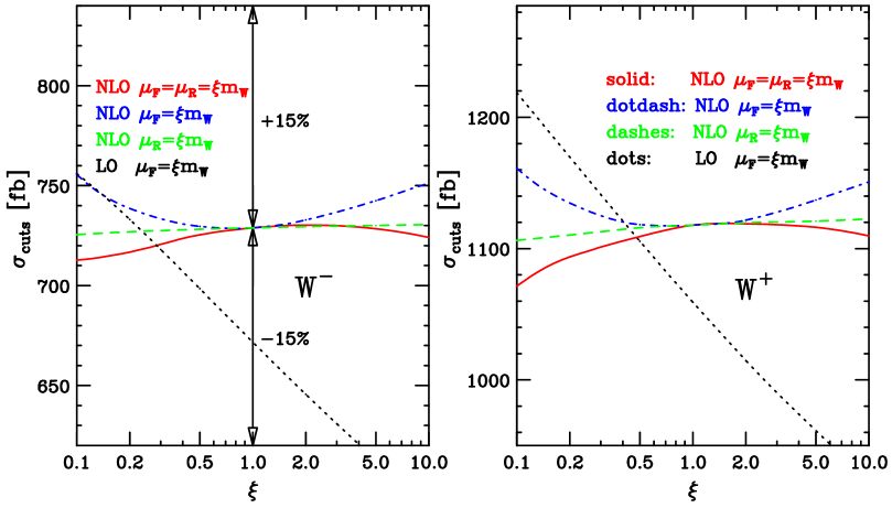
Figure 4: Scale dependence of the total cross section at LO and NLO within the cuts of Eqs. (4.1)–(4.4) for $W^{-}$ and $W^{+}$ production at the LHC. The decay branching ratio of the $W$ is included in the definition of the cross section, here and in all subsequent figures. The factorization scale $\mu_{F}$ and/or the renormalization scale $\mu_{R}$ have been taken as multiples of the vector-boson mass, $\xi\,m_{W}$, and $\xi$ is varied in the range $0.1<\xi<10$. The NLO curves are for $\mu_{F}=\mu_{R}=\xi m_{W}$ (solid red line), $\mu_{F}=m_{W}$ and $\mu_{R}=\xi\,m_{W}$ (dashed green line) and $\mu_{R}=m_{W}$ and $\mu_{F}$ variable (dot-dashed blue line). The dotted black curve shows the dependence of the LO cross section on the factorization scale. At this order, $\alpha_{s}(\mu_{R})$ does not enter.

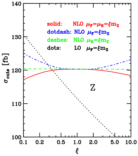
Figure 5: Same as Fig. 4, but for $Z$ production at the LHC, with the $Z\mbox{$\rightarrow$}\mu^{+}\mu^{-}$ branching ratio included in the definition of the cross section, here and in all subsequent figures.

Cross sections, within the cuts of Eqs. (4.1)–(4.4), are shown in Fig. 4, for $Wjj$ production, and in Fig. 5, for the $Zjj$ case. In both figures, the scale dependence of the LO and NLO cross sections is shown for fixed renormalization and factorization scales, $\mu_{R}$ and $\mu_{F}$, which are tied to the masses of the produced vector bosons $m_{V}$

$$\mu_{R}=\xi_{R}\,m_{V}\;,\qquad\qquad\mu_{F}=\xi_{F}\,m_{V}\;.$$ (4.5)

The LO cross sections only depend on $\mu_{F}=\xi\,m_{V}$. At NLO we show three cases: (a) $\xi_{F}=\xi_{R}=\xi$ (red solid line); (b) $\xi_{F}=\xi$, $\xi_{R}=1$ (blue dot-dashed line); and (c) $\xi_{R}=\xi$, $\xi_{F}=1$ (green dashed line). While the factorization-scale dependence of the LO result is sizable, the NLO cross sections are quite insensitive to scale variations: allowing a factor 2 variation in either directions, i.e., considering the range $0.5<\xi<2$, the NLO cross sections change by less than 1% in all cases.

As a second option, we have considered scales tied to the virtuality of the exchanged electroweak bosons. Specifically, independent scales $Q_{i}$ are determined as in Eqs. (2.2) and (2.5) for radiative corrections on the upper and on the lower quark line, and we set

$$\mu_{Fi}=\xi_{F}Q_{i}\;,\qquad\qquad\mu_{Ri}=\xi_{R}Q_{i}\;.$$ (4.6)

This choice is motivated by the picture of VBF as two independent deep-inelastic scattering type events, with independent radiative corrections on the two electroweak-boson vertices. Resulting $Vjj$ cross sections at NLO are about 1% lower for $\mu_{F}=\mu_{R}=Q_{i}$ than for $\mu_{F}=\mu_{R}=m_{V}$. In the following, we refer to the latter choice as the “$M$ scheme” while the choice $\mu_{F}=\mu_{R}=Q_{i}$ is called the “$Q$ scheme”. As we will see below, a residual NLO scale dependence of about 1%–2% is also typical for distributions, resulting in very stable NLO predictions for $Vjj$ cross sections.

In addition to these quite small scale uncertainties, we have estimated the error of the $W^{\pm}jj$ cross sections due to uncertainties in the determination of the PDFs. This error is determined by calculating the total $Wjj$ cross section, within the cuts of Eqs. (4.1)–(4.4), using two different sets of PDFs with errors, computed by the CTEQ [29] and MRST [33] Collaborations. Together with the PDF that gives the best fit to the data, the CTEQ6M set provides 40 PDFs, and the MRST2001E 30 PDFs, which correspond to extremal plus-minus variations in the directions of the error eigenvectors of the Hessian, in the space of the fitting parameters. To be on the conservative side, we have added the maximum deviations for each error eigenvector in quadrature, and we have found a total PDF uncertainty of $\pm 4\%$ with the CTEQ PDFs, and of roughly $\pm 2\%$ with the MRST set.

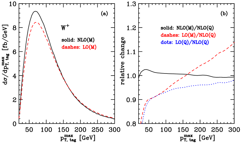
Figure 6: Transverse-momentum distribution of the highest-$p_{T}$ tagging jet in $W^{+}$ production at the LHC. In panel (a) the NLO result (solid black line) and the LO curve (dashed red line) are shown for the scale choice $\mu_{F}=\mu_{R}=m_{W}$ ($M$ scheme). In panel (b), we show the ratios of the NLO differential cross section in the $M$ scheme (solid black line), of the LO one in the $M$ scheme (dashed red line) and of the LO one in the $Q$ scheme (blue dotted line) to the NLO distribution in the $Q$ scheme, which is defined via the scale choice $\mu_{F}=\mu_{R}=Q_{i}$.

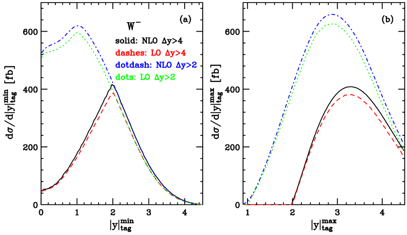
Figure 7: $W^{-}$ production cross section as a function of (a) the smaller and (b) the larger absolute value of the two tagging-jet rapidities. Results are shown for a rapidity separation between the two tagging jets greater than 2 and 4 (higher and lower pairs of curves, respectively). The LO cross section is always slightly below the NLO result. Due to the rapidity cut of Eq. (4.1), the distributions are truncated at $|y_{j}|=4.5$.

For precise comparisons with future LHC data, the residual theoretical error on the jet and lepton distributions must be estimated. As a first example, we show the transverse-momentum distribution of the highest-$p_{T}$ tagging jet for $W^{+}jj$ production in Fig. 6 (a): the shape of the $p_{T}$ distribution is fairly similar at LO (red dashed curve) and NLO (black solid line). Both curves were obtained with a scale choice of $\mu_{R}=\mu_{F}=m_{W}$. In the right-hand panel their ratio to the NLO curve with $\mu_{R}=\mu_{F}=Q_{i}$ is shown. The ratio of the two NLO distributions deviates from unity by 2% or less over the entire range, which, again, points to the small QCD dependence of our calculation.

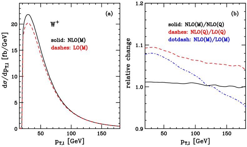
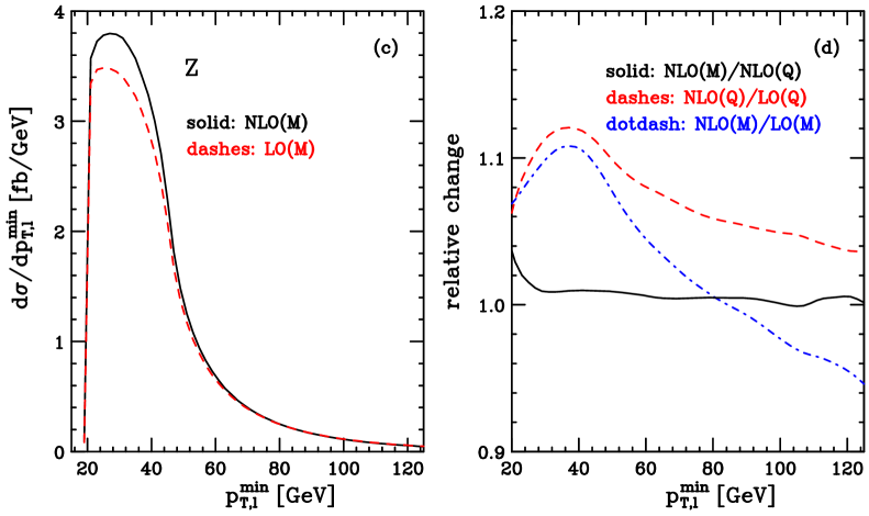
Figure 8: Transverse-momentum distributions of the charged final-state lepton in $W^{+}$ production [panels (a) and  (b)] and of the softest of the two final-state leptons in $Z$ production [panels (c) and (d)]. The solid black curves in panel (a) and (c) represent the NLO cross sections and the red dashed curves the LO ones, for scales $\mu_{R}=\mu_{F}=m_{V}$ ($M$ scheme). Panels (b) and (d) show the ratio of the NLO transverse-momentum distribution computed in the $M$ and $Q$ scheme (black solid line), and the $K$ factors in the $Q$ (red dashed line) and $M$ (blue dot-dashed line) schemes.

In contrast to the stability of the NLO result, the LO curves depend appreciably on the scale choice. The blue dotted line and the red dashed line in Fig. 6 (b) give the ratio of the LO curves for $\mu_{F}=Q_{i}$ and $\mu_{F}=m_{W}$, respectively, to the NLO result. The shape of the LO curves, in particular for a constant scale choice like $\mu_{F}=m_{W}$, is quite different from the more reliable NLO result. For transverse-momentum distributions we generally find that the “dynamical” scale choice $\mu_{F}=Q_{i}$, at LO, better reproduces the shape of the NLO distributions, and is thus preferable to a fixed scale. At NLO, or higher order, where the definition of the momentum transfer $Q_{i}$ becomes more problematic, the fixed-scale choice becomes more natural. However, because of the greater stability of the cross-section prediction, the scale selection also becomes less of a phenomenological issue.

Rapidity distributions of the two tagging jets are shown in Fig. 7, at LO and NLO, and for two choices of the rapidity-gap requirement, $\Delta y_{jj}>2$ and $\Delta y_{jj}>4$. The shapes of the rapidity distributions for the more central tagging jet, panel (a), and the more forward tagging jet, panel (b), are quite similar at LO and NLO. In fact, the $K$ factors for these distributions are fairly flat, and adequately described by a constant value of about 1.1. The results in Fig. 7 were obtained for a fixed scale $\mu_{F}=\mu_{R}=m_{W}$ and are for $W^{-}jj$ production. Curves for the $W^{+}jj$ and $Zjj$ cross sections are very similar in shape and show the preservation of shape between LO and NLO curves.

While tagging-jet distributions are quite similar for electroweak $Wjj$ and $Zjj$ events at the LHC, the presence of two charged leptons in the $Zjj$ case results in somewhat more noticeable differences. When considering changes in the lepton $p_{T}$ cut of Eq. (4.2), the transverse momentum of the softer lepton is critical for $Z$ production, while the single charged lepton must be considered for $Wjj$ events. These distributions are shown in Fig. 8 for $W^{+}$ production (top panels) and $Z$ production (bottom panels). At NLO the scale variations are again very small, at the 1% level, as demonstrated by the ratios of the NLO $p_{T}$ distributions for $\mu_{F}=\mu_{R}=m_{V}$ and $\mu_{F}=\mu_{R}=Q_{i}$ (solid black lines) in Fig. 8 (b, d). Varying either scales by a factor of 2 leads to the same conclusion of 1%–2% scale uncertainties for the NLO results. Comparing the LO predictions (dashed and dot-dashed curves) with the very precise NLO results shows theoretical errors of the order of 10%. Again, as for the jet $p_{T}$ distributions discussed earlier, the choice $\mu_{F}=Q_{i}$ is better for simulating the shape of the lepton $p_{T}$ distribution at LO. A fixed scale, $\mu_{F}=m_{V}$, predicts too steep a fall-off at large $p_{T}$. One should note, however, that for the electroweak $Vjj$ processes considered here, these differences are exceptionally small already at LO: the differences between the LO curves in Fig. 8 are of the order of 10% only.

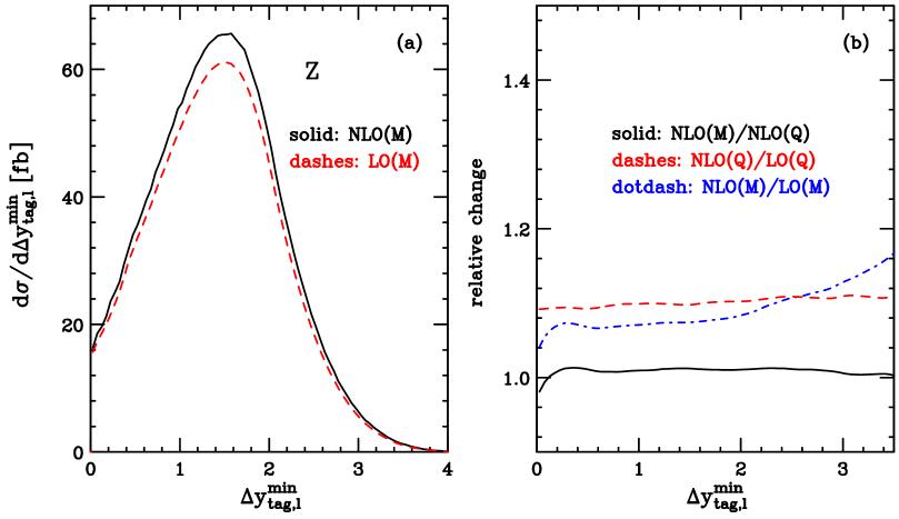
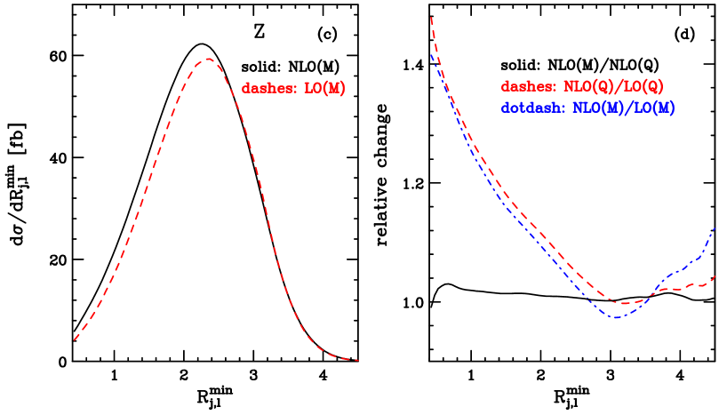
Figure 9: Angular correlations of leptons and jets in Z production. Panels (a) and (b) show the minimum rapidity separation between the two leptons and the two tagging jets. Panels (c) and (d) are for the minimum rapidity-azimuthal angle separations between the leptons and any reconstructed jets (not necessarily the two tagging jets). The NLO differential cross sections are shown in black solid lines, while the LO ones are displayed as red dashed lines. Scales are fixed in the $M$ scheme. Panels (b) and (d) show the ratio between the two NLO differential cross sections in the $M$ and $Q$ scheme (solid black lines) and their respective $K$ factors.

In contrast to the lepton transverse-momentum distributions described above, the shape of the lepton-rapidity distributions is virtually unaffected by the NLO corrections: an overall constant $K$ factor is sufficient to describe NLO effects. Larger changes are found when considering angular correlations of the leptons and jets, which we show for $Zjj$ production in Fig. 9. The top panels show the minimal rapidity between any of the two leptons and the two tagging jets, $\Delta y_{{\rm tag},l}^{\rm min}$. As before, the tagging jets are taken as the two highest transverse-momentum jets in the event ($p_{T}$ selection). The two bottom panels show the minimal separation in the rapidity-azimuthal angle plane of the two leptons from any jet (not necessarily the two tagging jets) in the event, $R_{j,l}^{\rm min}$. In both cases, the two scale choices for the NLO result show excellent agreement (black solid lines in Fig. 9 (b, d)). However, the dynamical $K$ factors

$$K(x)=\frac{d\sigma_{NLO}/dx}{d\sigma_{LO}/dx}$$ (4.7)

for $x=\Delta y_{{\rm tag},l}^{\rm min}$ and $x=R_{j,l}^{\rm min}$ show qualitatively different behavior. While $K(\Delta y_{{\rm tag},l}^{\rm min})$ is fairly constant, i.e., the shape of the distribution is well described by the LO approximation, the minimal lepton-jet separation, $d\sigma/dR_{j,l}^{\rm min}$, shifts noticeably to smaller values at NLO. This behavior was to be expected, since additional parton emission in the higher-order calculation reduces lepton isolation. What is remarkable, then, is that the selection of the tagging jets as the two highest-$p_{T}$ jets does not affect the lepton-tagging jet separation. As for the Higgs boson case [15], this selection of the tagging jets provides excellent correspondence of the LO- and NLO-event topology.

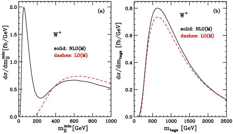
Figure 10: Dijet invariant-mass distributions for $W^{+}$ production, with scales in the $M$ scheme. Shown are (a) the minimum dijet invariant-mass distribution for any final-state reconstructed jets (not necessarily the two tagging jets) and (b) the invariant mass of the two tagging jets. NLO results are shown in solid black lines, while the red dashed lines are for LO distributions.

In order to stress this point we show dijet invariant-mass distributions for the reconstructed jets (not necessarily the two tagging jets) for $W^{+}jj$ events at LO (red dashed lines) and at NLO (solid black lines) in Fig. 10. The distribution with respect to the minimal dijet invariant mass in the event is shown in Fig. 10 (a) while Fig. 10 (b) uses the invariant mass of the two tagging jets, $m_{\rm tags}$. At LO, there are only two final-state quarks of $p_{T}>20$ GeV in each event and, hence, the two curves are identical. At NLO, additional parton emission provides for soft third jets which form low invariant-mass pairs with one of the tagging jets, and this pair shows up as a low-mass peak in $d\sigma/dm_{jj}^{\rm min}$. Generic selections of the two tagging jets in a multijet environment tend to pick up some of these low-mass pairs and lead to substantial differences in the invariant-mass distribution of the two tagging jets at LO and at NLO. The $p_{T}$ selection of tagging jets, which we have used throughout and for which results are shown in Fig. 10 (b), is remarkable in that it preserves the shape of the tagging jet invariant-mass distribution, $d\sigma/dm_{\rm tags}$, when going from LO to NLO.

5 Conclusions

Vector-boson fusion at the LHC represents a class of electroweak processes which are under excellent control perturbatively. This has been known for some time for the most interesting process in this class: Higgs boson production via VBF has a modest $K$ factor of about 1.05 for the inclusive production cross section [14] and this result also holds when applying realistic acceptance cuts [15].

In the present paper, we have extended this result to the electroweak production of $W$ and $Z$ plus two jets, when the final-state particles are in a kinematic configuration typical of VBF events. More precisely, we have calculated the NLO QCD corrections to electroweak production of $\ell\nu_{\ell}jj$ and $\ell^{+}\ell^{-}jj$ at LHC, and we have implemented them in a fully-flexible NLO Monte Carlo program. $K$ factors are of the same size as for the Higgs boson production process, typically ranging between 1.0 and 1.1 for most distributions. What is more important is the stability of the NLO result: residual scale dependence is at the 2% level or below. This is smaller than the present parton-distribution-function uncertainties, which we have calculated for the $W^{\pm}jj$ cross sections. We estimate 4% PDF errors using CTEQ6M parton distributions and roughly half that size using MRST2001E PDFs.

Given the excellent theoretical control which we now have for EW $Vjj$ production, these processes can be used as testing grounds for Higgs boson production in VBF: techniques should be developed to measure hadronic properties, like forward-jet tagging efficiencies or central-jet-veto probabilities, in $Wjj$ or $Zjj$ production at the LHC and to extrapolate these results to Higgs boson production, thus reducing the systematic errors for Higgs boson coupling measurements. We leave such applications for the future.

A Virtual corrections

In this appendix, we give the expression for the finite, reduced amplitude $\tilde{\cal M}_{\tau}(q_{1},q_{2})$ that appears in Eqs. (2.5) and (2.6), in terms of $\tilde{B}_{0}$, $\tilde{C}_{0}$ and $\tilde{D}_{ij}$ functions. Here $\tilde{B}_{0}$, $\tilde{C}_{0}$ and $\tilde{D}_{ij}$ are the finite parts of the Passarino-Veltman $B_{0}$, $C_{0}$ and $D_{ij}$ functions [34], and are given explicitly below. We have also derived $\tilde{\cal M}_{\tau}(q_{1},q_{2})$ in terms of $\tilde{B}_{0}$, $\tilde{C}_{0}$ and $\tilde{D}_{0}$ functions, but do not show this expression here, due to its length. We write

$$\tilde{\cal M}_{\tau}(q_{1},q_{2})=\overline{\psi}(k_{2})\left[c_{1}\epsilon\hskip-4.05904pt\hbox to4.05904pt{\hss$/$\hss}_{1}+c_{2}\epsilon\hskip-4.05904pt\hbox to4.05904pt{\hss$/$\hss}_{2}+c_{q}\left(q\hskip-4.8229pt\hbox to4.8229pt{\hss$/$\hss}_{1}-q\hskip-4.8229pt\hbox to4.8229pt{\hss$/$\hss}_{2}\right)+c_{b}\epsilon\hskip-4.05904pt\hbox to4.05904pt{\hss$/$\hss}_{2}\left(k\hskip-5.52084pt\hbox to5.52084pt{\hss$/$\hss}_{2}+q\hskip-4.8229pt\hbox to4.8229pt{\hss$/$\hss}_{2}\right)\epsilon\hskip-4.05904pt\hbox to4.05904pt{\hss$/$\hss}_{1}\right]\frac{1+\tau\gamma_{5}}{2}\psi(k_{1})\,,$$ (A.1)

where $\epsilon_{1}=\epsilon_{1}(q_{1})$ and $\epsilon_{2}=\epsilon_{2}(q_{2})$ are the effective polarization vectors of the two electroweak gauge bosons. The coefficient function $c_{1}=c_{1}(q_{1},q_{2})$ is given by

$$c_{1} = 2\epsilon_{2}\cdot k_{2}T_{\epsilon}\left(q_{2}^{2},t\right)-2\left[\tilde{D}_{12}(k_{2},q_{2},q_{1})+\tilde{D}_{24}(k_{2},q_{2},q_{1})\right]\epsilon_{2}\cdot k_{2}\left(q_{1}^{2}+q_{2}^{2}-3s-4t\right)$$ (A.2)

$$- 2\left[\tilde{D}_{12}(k_{2},q_{2},q_{1})-\tilde{D}_{24}(k_{2},q_{2},q_{1})\right]\epsilon_{2}\cdot q_{1}\left(q_{2}^{2}-t\right)$$

$$+ 4\Bigl{[}-\tilde{D}_{11}(k_{2},q_{2},q_{1})\epsilon_{2}\cdot k_{2}s-\tilde{D}_{12}(k_{2},q_{2},q_{1})\epsilon_{2}\cdot k_{1}t+\tilde{D}_{13}(k_{2},q_{2},q_{1})\epsilon_{2}\cdot k_{2}\left(q_{2}^{2}-s-t\right)$$

$$+ \tilde{D}_{13}(k_{2},q_{2},q_{1})\epsilon_{2}\cdot q_{1}q_{2}^{2}-\tilde{D}_{21}(k_{2},q_{2},q_{1})\epsilon_{2}\cdot k_{2}s-\tilde{D}_{22}(k_{2},q_{2},q_{1})\epsilon_{2}\cdot k_{2}t$$

$$- \tilde{D}_{22}(k_{2},q_{2},q_{1})\epsilon_{2}\cdot q_{1}q_{2}^{2}+\tilde{D}_{23}(k_{2},q_{2},q_{1})\epsilon_{2}\cdot k_{2}q_{1}^{2}+\tilde{D}_{25}(k_{2},q_{2},q_{1})\epsilon_{2}\cdot k_{2}\left(q_{2}^{2}-s-2t\right)$$

$$- \tilde{D}_{26}(k_{2},q_{2},q_{1})\epsilon_{2}\cdot k_{2}\left(q_{2}^{2}-s-t\right)+\tilde{D}_{26}(k_{2},q_{2},q_{1})\epsilon_{2}\cdot q_{1}t+2\tilde{D}_{27}(k_{2},q_{2},q_{1})\epsilon_{2}\cdot q_{1}$$

$$- \tilde{D}_{32}(k_{2},q_{2},q_{1})\epsilon_{2}\cdot k_{2}q_{2}^{2}-\tilde{D}_{34}(k_{2},q_{2},q_{1})\epsilon_{2}\cdot k_{2}(q_{2}^{2}-t)$$

$$+ \tilde{D}_{36}(k_{2},q_{2},q_{1})\epsilon_{2}\cdot k_{2}\left(2q_{2}^{2}-t\right)+\tilde{D}_{37}(k_{2},q_{2},q_{1})\epsilon_{2}\cdot k_{2}q_{1}^{2}$$

$$+ \tilde{D}_{35}(k_{2},q_{2},q_{1})\epsilon_{2}\cdot k_{2}\left(q_{2}^{2}-s-t\right)+\tilde{D}_{38}(k_{2},q_{2},q_{1})\epsilon_{2}\cdot k_{2}\left(q_{1}^{2}+q_{2}^{2}-s\right)$$

$$- \tilde{D}_{39}(k_{2},q_{2},q_{1})\epsilon_{2}\cdot k_{2}q_{1}^{2}-\tilde{D}_{310}(k_{2},q_{2},q_{1})\epsilon_{2}\cdot k_{2}\left(q_{1}^{2}+2q_{2}^{2}-2s-t\right)$$

$$- 4\tilde{D}_{311}(k_{2},q_{2},q_{1})\epsilon_{2}\cdot k_{2}+6\tilde{D}_{312}(k_{2},q_{2},q_{1})\epsilon_{2}\cdot k_{2}+2\tilde{D}_{313}(k_{2},q_{2},q_{1})\epsilon_{2}\cdot q_{1}\Bigl{]}\;,$$

where

$$T_{\epsilon}\left(q^{2},t\right)=\frac{1}{t-q^{2}}\left\{\left[\tilde{B}_{0}(t)-\tilde{B}_{0}(q^{2})\right]\frac{2t+3q^{2}}{t-q^{2}}+2\tilde{B}_{0}(q^{2})+1-2q^{2}\tilde{C}_{0}(q^{2},t)\right\}$$ (A.3)

is defined in terms of the finite parts of the $B_{0}$ and $C_{0}$ functions

$$\tilde{B}_{0}(q^{2})=2-\ln\frac{q^{2}+i0^{+}}{s}$$ (A.4)

and

$$\tilde{C}_{0}(q^{2},t)=\frac{1}{2(t-q^{2})}\biggl{(}\ln^{2}\frac{q^{2}+i0^{+}}{s}-\ln^{2}\frac{t+i0^{+}}{s}\biggr{)}\,.$$ (A.5)

These expressions are obtained by pulling a common factor $\Gamma(1+\epsilon)(-s)^{-\epsilon}\equiv{\Gamma(1+\epsilon)}/(Q^{2})^{\epsilon}$ out of all amplitudes and Passarino-Veltman functions, e.g.,

$$B_{0}(q^{2}) = \int\frac{d^{d}k}{i\pi^{d/2}}\frac{1}{k^{2}(k+q)^{2}}=\frac{\Gamma(1+\epsilon)}{\epsilon}\frac{\Gamma(1-\epsilon)^{2}}{\Gamma(2-2\epsilon)}(-q^{2}-i0^{+})^{-\epsilon}$$ (A.6)

$$= \frac{\Gamma(1+\epsilon)}{\left(-s\right)^{\epsilon}}\left[\frac{1}{\epsilon}+2-\ln\frac{q^{2}+i0^{+}}{s}+{\cal O}\left(\epsilon\right)\right]=\frac{\Gamma(1+\epsilon)}{\left(Q^{2}\right)^{\epsilon}}\left[\frac{1}{\epsilon}+\tilde{B}_{0}(q^{2})+{\cal O}\left(\epsilon\right)\right]\,.\phantom{aaaaa}$$

For the other coefficient functions $c_{i}=c_{i}(q_{1},q_{2})$ we find

$$c_{2} = -2\left[\tilde{D}_{12}(k_{2},q_{2},q_{1})+\tilde{D}_{24}(k_{2},q_{2},q_{1})\right]\left[\epsilon_{1}\cdot k_{2}\left(q_{1}^{2}+q_{2}^{2}-s-2t\right)+\epsilon_{1}\cdot q_{2}\left(q_{2}^{2}-s-3t\right)\right]$$ (A.7)

$$+ 4\Big{[}\tilde{D}_{13}(k_{2},q_{2},q_{1})\epsilon_{1}\cdot k_{2}q_{1}^{2}-\tilde{D}_{13}(k_{2},q_{2},q_{1})\epsilon_{1}\cdot k_{1}(2s+t)+\tilde{D}_{22}(k_{2},q_{2},q_{1})\epsilon_{1}\cdot k_{1}q_{2}^{2}$$

$$- \tilde{D}_{23}(k_{2},q_{2},q_{1})\epsilon_{1}\cdot k_{2}t+\tilde{D}_{23}(k_{2},q_{2},q_{1})\epsilon_{1}\cdot q_{2}\left(q_{1}^{2}-t\right)-\tilde{D}_{24}(k_{2},q_{2},q_{1})\epsilon_{1}\cdot k_{1}q_{2}^{2}$$

$$+ \tilde{D}_{25}(k_{2},q_{2},q_{1})\epsilon_{1}\cdot k_{2}q_{1}^{2}+\tilde{D}_{25}(k_{2},q_{2},q_{1})\epsilon_{1}\cdot k_{1}\left(q_{2}^{2}-2s-t\right)+\tilde{D}_{26}(k_{2},q_{2},q_{1})\epsilon_{1}\cdot k_{2}t$$

$$- \tilde{D}_{26}(k_{2},q_{2},q_{1})\epsilon_{1}\cdot k_{1}\left(q_{1}^{2}-s\right)-2\tilde{D}_{27}(k_{2},q_{2},q_{1})\epsilon_{1}\cdot q_{2}+\tilde{D}_{33}(k_{2},q_{2},q_{1})\epsilon_{1}\cdot k_{2}q_{1}^{2}$$

$$+ \tilde{D}_{33}(k_{2},q_{2},q_{1})\epsilon_{1}\cdot q_{2}q_{1}^{2}+\tilde{D}_{37}(k_{2},q_{2},q_{1})\epsilon_{1}\cdot k_{1}\left(q_{2}^{2}-s-t\right)+\tilde{D}_{38}(k_{2},q_{2},q_{1})\epsilon_{1}\cdot k_{1}q_{2}^{2}$$

$$- \tilde{D}_{39}(k_{2},q_{2},q_{1})\epsilon_{1}\cdot k_{1}\left(q_{1}^{2}+q_{2}^{2}-s\right)-\tilde{D}_{310}(k_{2},q_{2},q_{1})\epsilon_{1}\cdot k_{1}\left(q_{2}^{2}-t\right)$$

$$+ 2\tilde{D}_{311}(k_{2},q_{2},q_{1})\epsilon_{1}\cdot k_{2}+2\tilde{D}_{312}(k_{2},q_{2},q_{1})\epsilon_{1}\cdot q_{2}-6\tilde{D}_{313}(k_{2},q_{2},q_{1})\epsilon_{1}\cdot k_{1}\Big{]}$$

$$+ 2\epsilon_{1}\cdot k_{1}T_{\epsilon}\left(q_{1}^{2},t\right)\;,$$

$$c_{q} = \left[\tilde{D}_{12}(k_{2},q_{2},q_{1})+\tilde{D}_{24}(k_{2},q_{2},q_{1})\right]\epsilon_{1}\cdot\epsilon_{2}s+2\Big{[}4\tilde{D}_{12}(k_{2},q_{2},q_{1})\epsilon_{2}\cdot k_{2}\epsilon_{1}\cdot k_{2}$$ (A.8)

$$+ 3\tilde{D}_{12}(k_{2},q_{2},q_{1})\epsilon_{2}\cdot k_{2}\epsilon_{1}\cdot q_{2}+\tilde{D}_{12}(k_{2},q_{2},q_{1})\epsilon_{2}\cdot q_{1}\epsilon_{1}\cdot k_{2}-4\tilde{D}_{13}(k_{2},q_{2},q_{1})\epsilon_{2}\cdot k_{2}\epsilon_{1}\cdot k_{2}$$

$$- 2\tilde{D}_{13}(k_{2},q_{2},q_{1})\epsilon_{2}\cdot k_{2}\epsilon_{1}\cdot q_{2}-2\tilde{D}_{13}(k_{2},q_{2},q_{1})\epsilon_{2}\cdot q_{1}\epsilon_{1}\cdot k_{2}-\tilde{D}_{13}(k_{2},q_{2},q_{1})\epsilon_{1}\cdot\epsilon_{2}s$$

$$+ 2\tilde{D}_{22}(k_{2},q_{2},q_{1})\epsilon_{2}\cdot k_{2}\epsilon_{1}\cdot q_{2}-\tilde{D}_{22}(k_{2},q_{2},q_{1})\epsilon_{1}\cdot\epsilon_{2}t-2\tilde{D}_{23}(k_{2},q_{2},q_{1})\epsilon_{2}\cdot q_{1}\epsilon_{1}\cdot k_{2}$$

$$- 2\tilde{D}_{23}(k_{2},q_{2},q_{1})\epsilon_{2}\cdot q_{1}\epsilon_{1}\cdot q_{2}-\tilde{D}_{23}(k_{2},q_{2},q_{1})\epsilon_{1}\cdot\epsilon_{2}t+6\tilde{D}_{24}(k_{2},q_{2},q_{1})\epsilon_{2}\cdot k_{2}\epsilon_{1}\cdot k_{2}$$

$$+ 3\tilde{D}_{24}(k_{2},q_{2},q_{1})\epsilon_{2}\cdot k_{2}\epsilon_{1}\cdot q_{2}+\tilde{D}_{24}(k_{2},q_{2},q_{1})\epsilon_{2}\cdot q_{1}\epsilon_{1}\cdot k_{2}-6\tilde{D}_{25}(k_{2},q_{2},q_{1})\epsilon_{2}\cdot k_{2}\epsilon_{1}\cdot k_{2}$$

$$- 2\tilde{D}_{25}(k_{2},q_{2},q_{1})\epsilon_{2}\cdot k_{2}\epsilon_{1}\cdot q_{2}-2\tilde{D}_{25}(k_{2},q_{2},q_{1})\epsilon_{2}\cdot q_{1}\epsilon_{1}\cdot k_{2}-\tilde{D}_{25}(k_{2},q_{2},q_{1})\epsilon_{1}\cdot\epsilon_{2}s$$

$$- 4\tilde{D}_{26}(k_{2},q_{2},q_{1})\epsilon_{2}\cdot k_{2}\epsilon_{1}\cdot q_{2}+4\tilde{D}_{26}(k_{2},q_{2},q_{1})\epsilon_{2}\cdot q_{1}\epsilon_{1}\cdot k_{2}+2\tilde{D}_{26}(k_{2},q_{2},q_{1})\epsilon_{2}\cdot q_{1}\epsilon_{1}\cdot q_{2}$$

$$+ \tilde{D}_{26}(k_{2},q_{2},q_{1})\epsilon_{1}\cdot\epsilon_{2}\left(s+2t\right)-\tilde{D}_{32}(k_{2},q_{2},q_{1})\epsilon_{1}\cdot\epsilon_{2}q_{2}^{2}+\tilde{D}_{33}(k_{2},q_{2},q_{1})\epsilon_{1}\cdot\epsilon_{2}q_{1}^{2}$$

$$+ 2\tilde{D}_{34}(k_{2},q_{2},q_{1})\epsilon_{2}\cdot k_{2}\epsilon_{1}\cdot k_{2}-2\tilde{D}_{35}(k_{2},q_{2},q_{1})\epsilon_{2}\cdot k_{2}\epsilon_{1}\cdot k_{2}$$

$$+ \tilde{D}_{36}(k_{2},q_{2},q_{1})\epsilon_{1}\cdot\epsilon_{2}\left(q_{2}^{2}-t\right)-2\tilde{D}_{37}(k_{2},q_{2},q_{1})\epsilon_{2}\cdot q_{1}\epsilon_{1}\cdot k_{2}$$

$$+ 2\tilde{D}_{36}(k_{2},q_{2},q_{1})\epsilon_{2}\cdot k_{2}\epsilon_{1}\cdot q_{2}+\tilde{D}_{37}(k_{2},q_{2},q_{1})\epsilon_{1}\cdot\epsilon_{2}\left(q_{2}^{2}-s-t\right)$$

$$+ 2\tilde{D}_{38}(k_{2},q_{2},q_{1})\epsilon_{2}\cdot q_{1}\epsilon_{1}\cdot q_{2}+\tilde{D}_{38}(k_{2},q_{2},q_{1})\epsilon_{1}\cdot\epsilon_{2}\left(q_{1}^{2}+2q_{2}^{2}-s\right)$$

$$- 2\tilde{D}_{39}(k_{2},q_{2},q_{1})\epsilon_{2}\cdot q_{1}\epsilon_{1}\cdot q_{2}-\tilde{D}_{39}(k_{2},q_{2},q_{1})\epsilon_{1}\cdot\epsilon_{2}\left(2q_{1}^{2}+q_{2}^{2}-s\right)$$

$$- 2\tilde{D}_{310}(k_{2},q_{2},q_{1})\epsilon_{2}\cdot k_{2}\epsilon_{1}\cdot q_{2}+2\tilde{D}_{310}(k_{2},q_{2},q_{1})\epsilon_{2}\cdot q_{1}\epsilon_{1}\cdot k_{2}$$

$$- \tilde{D}_{310}(k_{2},q_{2},q_{1})\epsilon_{1}\cdot\epsilon_{2}\left(2q_{2}^{2}-s-2t\right)+4\tilde{D}_{312}(k_{2},q_{2},q_{1})\epsilon_{1}\cdot\epsilon_{2}$$

$$- 4\tilde{D}_{313}(k_{2},q_{2},q_{1})\epsilon_{1}\cdot\epsilon_{2}\Big{]}\;,$$

$$c_{b} = -2\Big{\{}\left[\tilde{D}_{36}(k_{2},q_{2},q_{1})+\tilde{D}_{37}(k_{2},q_{2},q_{1})-2\tilde{D}_{310}(k_{2},q_{2},q_{1})\right]\left(q_{2}^{2}-t\right)$$ (A.9)

$$+ \tilde{D}_{38}(k_{2},q_{2},q_{1})\left(q_{1}^{2}+2q_{2}^{2}\right)-\tilde{D}_{39}(k_{2},q_{2},q_{1})\left(2q_{1}^{2}+q_{2}^{2}\right)\Big{\}}-2\Big{[}\tilde{D}_{0}(k_{2},q_{2},q_{1})$$

$$+ \tilde{D}_{11}(k_{2},q_{2},q_{1})+\tilde{D}_{12}(k_{2},q_{2},q_{1})-2\tilde{D}_{13}(k_{2},q_{2},q_{1})+\tilde{D}_{24}(k_{2},q_{2},q_{1})-\tilde{D}_{25}(k_{2},q_{2},q_{1})$$

$$+ \tilde{D}_{26}(k_{2},q_{2},q_{1})-\tilde{D}_{37}(k_{2},q_{2},q_{1})-\tilde{D}_{38}(k_{2},q_{2},q_{1})+\tilde{D}_{39}(k_{2},q_{2},q_{1})+\tilde{D}_{310}(k_{2},q_{2},q_{1})\Big{]}s$$

$$+ 2\Big{\{}\left[\tilde{D}_{22}(k_{2},q_{2},q_{1})+\tilde{D}_{23}(k_{2},q_{2},q_{1})-2\tilde{D}_{26}(k_{2},q_{2},q_{1})\right]t-2\tilde{D}_{27}(k_{2},q_{2},q_{1})$$

$$+ \tilde{D}_{32}(k_{2},q_{2},q_{1})q_{2}^{2}-\tilde{D}_{33}(k_{2},q_{2},q_{1})q_{1}^{2}-6\left(\tilde{D}_{312}(k_{2},q_{2},q_{1})-\tilde{D}_{313}(k_{2},q_{2},q_{1})\right)\Big{\}}$$

$$- \frac{1}{t}\left[T_{b}(q_{1}^{2},t)+T_{b}(q_{2}^{2},t)+\tilde{B}_{0}(t)-5+\frac{\pi^{2}}{3}\;\right]\,,$$

with

$$T_{b}(q^{2},t)=\frac{1}{t-q^{2}}\left\{2q^{2}\left[\tilde{B}_{0}(t)-\tilde{B}_{0}(q^{2})\right]+t\tilde{B}_{0}(t)-q^{2}\tilde{B}_{0}(q^{2})\right\}-2q^{2}\tilde{C}_{0}(q^{2},t)\,.$$ (A.10)

For the crossed function $\tilde{\cal M}(q_{2},q_{1})$, the same expressions as above apply, with the obvious interchange $q_{1}\leftrightarrow q_{2}$, $\epsilon_{1}\leftrightarrow\epsilon_{2}$, and $t\,\mbox{$\rightarrow$}\,u$.

The finite part of the $D_{0}$ function is defined by

$$\tilde{D}_{0}(k_{2},q_{2},q_{1})=\frac{1}{2st}\left[\ln^{2}\frac{q_{1}^{2}q_{2}^{2}}{t^{2}}+4\;{\rm Li}_{2}\left(1-\frac{t}{q_{1}^{2}}\right)+4\;{\rm Li}_{2}\left(1-\frac{t}{q_{2}^{2}}\right)-\frac{\pi^{2}}{3}\right]\;.$$ (A.11)

This expression is well defined when all invariants, $q_{1}^{2}$, $q_{2}^{2}$ and $t$, are space-like. In our application, we always have one space-like and one time-like weak boson, i.e., exactly one of the two quotients $t/q_{i}^{2}$ is positive. In the other quotient simply replace the time-like invariant by $t\,\mbox{$\rightarrow$}\,t+i0^{+}$ or $q_{i}^{2}\,\mbox{$\rightarrow$}\,q_{i}^{2}+i0^{+}$, as in Eqs. (A.4) and (A.5).

The remaining finite $\tilde{D}_{ij}$ functions are obtained from the above expressions for the $\tilde{B}_{0}$, $\tilde{C}_{0}$, and $\tilde{D}_{0}$ functions with the usual Passarino-Veltman recursion relations given in Ref. [34], adapted to the Bjorken-Drell metric, $q_{i}^{2}>0$ for a time-like momentum $q_{i}$. In these recursion relations we need the additional finite $\tilde{B}_{0}$ and $\tilde{C}_{0}$ functions

$$\tilde{B}_{0}(0) = 0\;,$$ (A.12)

$$\tilde{C}_{0}(k_{2},q_{1}+q_{2}) = \tilde{C}_{0}(s,0,0)=\frac{1}{s}\frac{\pi^{2}}{6}\;,$$ (A.13)

while

$$\tilde{C}_{0}(q_{1},q_{2})=C_{0}(q_{1}^{2},q_{2}^{2},s)$$ (A.14)

is the infrared- and ultraviolet-finite $C_{0}$ function for massless internal propagators but with nonzero invariants $q_{1}^{2}$, $q_{2}^{2}$ and $s$.

References

• [1] ATLAS Collaboration, ATLAS TDR, Report No. CERN/LHCC/99-15 (1999); E. Richter-Was and M. Sapinski, Acta Phys. Pol. B 30, 1001 (1999); B. P. Kersevan and E. Richter-Was, Eur. Phys. J. C 25, 379 (2002) [arXiv:hep-ph/0203148].
• [2] G. L. Bayatian et al., CMS Technical Proposal, Report No. CERN/LHCC/94-38x (1994); R. Kinnunen and D. Denegri, CMS Note No. 1997/057; R. Kinnunen and A. Nikitenko, Report No. CMS TN/97-106; R. Kinnunen and D. Denegri, arXiv:hep-ph/9907291; V. Drollinger, T. Müller and D. Denegri, arXiv:hep-ph/0111312.
• [3] D. Zeppenfeld, R. Kinnunen, A. Nikitenko and E. Richter-Was, Phys. Rev. D 62, 013009 (2000) [arXiv:hep-ph/0002036]; D. Zeppenfeld, in Proc. of the APS/DPF/DPB Summer Study on the Future of Particle Physics, Snowmass, 2001 edited by N. Graf, eConf C010630, p. 123 (2001) [arXiv:hep-ph/0203123]; A. Belyaev and L. Reina, JHEP 0208, 041 (2002) [arXiv:hep-ph/0205270].
• [4] D. L. Rainwater, arXiv:hep-ph/9908378.
• [5] J. Campbell and R. K. Ellis, Phys. Rev. D 65, 113007 (2002) [arXiv:hep-ph/0202176]; J. Campbell, R. K. Ellis and D. Rainwater, Phys. Rev. D 68, 094021 (2003) [arXiv:hep-ph/0308195].
• [6] H. Chehime and D. Zeppenfeld, Phys. Rev. D 47, 3898 (1993).
• [7] D. Rainwater, R. Szalapski and D. Zeppenfeld, Phys. Rev. D 54, 6680 (1996) [arXiv:hep-ph/9605444].
• [8] V. A. Khoze, M. G. Ryskin, W. J. Stirling and P. H. Williams, Eur. Phys. J. C 26, 429 (2003) [arXiv:hep-ph/0207365].
• [9] U. Baur and D. Zeppenfeld, arXiv:hep-ph/9309227.
• [10] D. Rainwater, D. Zeppenfeld and K. Hagiwara, Phys. Rev. D 59, 014037 (1999) [arXiv:hep-ph/9808468]; T. Plehn, D. Rainwater and D. Zeppenfeld, Phys. Rev. D 61, 093005 (2000) [arXiv:hep-ph/9911385]; S. Asai et al., Report No. ATL-PHYS-2003-005.
• [11] D. Rainwater and D. Zeppenfeld, Phys. Rev. D 60, 113004 (1999) [Erratum-ibid. D 61, 099901 (2000)] [arXiv:hep-ph/9906218]; N. Kauer, T. Plehn, D. Rainwater and D. Zeppenfeld, Phys. Lett. B 503, 113 (2001) [arXiv:hep-ph/0012351]; C. M. Buttar, R. S. Harper and K. Jakobs, Report No. ATL-PHYS-2002-033; K. Cranmer et al., Report No. ATL-PHYS-2003-002 and Report No. ATL-PHYS-2003-007; S. Asai et al., Report No. ATL-PHYS-2003-005.
• [12] O. J. Eboli and D. Zeppenfeld, Phys. Lett. B 495, 147 (2000) [arXiv:hep-ph/0009158]; B. Di Girolamo, A. Nikitenko, L. Neukermans, K. Mazumdar and D. Zeppenfeld, in arXiv:hep-ph/0203056.
• [13] D. G. Charlton, arXiv:hep-ex/0110086. The LEP Electroweak Working Group: http://lepewwg.web.cern.ch/LEPEWWG.
• [14] T. Han, G. Valencia and S. Willenbrock, Phys. Rev. Lett.  69, 3274 (1992) [arXiv:hep-ph/9206246].
• [15] T. Figy, C. Oleari and D. Zeppenfeld, Phys. Rev. D 68, 073005 (2003) [arXiv:hep-ph/0306109].
• [16] F. Boudjema et al., arXiv:hep-ph/9601224.
• [17] T. Stelzer and W. F. Long, Comput. Phys. Commun.  81, 357 (1994) [arXiv:hep-ph/9401258]; F. Maltoni and T. Stelzer, JHEP 0302, 027 (2003) [arXiv:hep-ph/0208156].
• [18] K. Hagiwara and D. Zeppenfeld, Nucl. Phys. B274, 1 (1986); K. Hagiwara and D. Zeppenfeld, Nucl. Phys.  B313, 560 (1989).
• [19] S. Catani and M. H. Seymour, Nucl. Phys.  B485, 291 (1997) [Erratum-ibid.  B510, 503 (1997)] [arXiv:hep-ph/9605323].
• [20] Warren Siegel, Phys. Lett. B 84, 193 (1979); Warren Siegel, Phys. Lett. B 94, 37 (1980).
• [21] V. Ilyin, private communication.
• [22] G. P. Lepage, J. Comput. Phys. 27, 192 (1978).
• [23] See, e.g., E. N. Argyres et al., Phys. Lett. B 358, 339 (1995) [arXiv:hep-ph/9507216].
• [24] U. Baur, J. A. Vermaseren and D. Zeppenfeld, Nucl. Phys.  B375, 3 (1992).
• [25] A. Denner, S. Dittmaier, M. Roth and D. Wackeroth, Nucl. Phys.  B560, 33 (1999) [arXiv:hep-ph/9904472].
• [26] See, e.g., G. Lopez Castro, J.L.M. Lucio and J. Pestieau, Mod. Phys. Lett. A6, 3679 (1991); M. Nowakowski and A. Pilaftsis, Z. Phys. C60, 121 (1993); U. Baur and D. Zeppenfeld, Phys. Rev. Lett.  75, 1002 (1995) [arXiv:hep-ph/9503344], and references therein.
• [27] K. Hagiwara, R. D. Peccei, D. Zeppenfeld and K. Hikasa, Nucl. Phys.  B282, 253 (1987).
• [28] K. Hagiwara, D. Zeppenfeld and S. Komamiya, Z. Phys. C 29, 115 (1985); B. A. Kniehl, Phys. Lett. B 254, 267 (1991).
• [29] J. Pumplin, D. R. Stump, J. Huston, H. L. Lai, P. Nadolsky and W. K. Tung, JHEP 0207, 012 (2002) [arXiv:hep-ph/0201195].
• [30] K. Hagiwara et al. [Particle Data Group Collaboration], Phys. Rev. D 66, 010001 (2002).
• [31] S. Catani, Yu. L. Dokshitzer and B. R. Webber, Phys. Lett. B 285 291 (1992); S. Catani, Yu. L. Dokshitzer, M. H. Seymour and B. R. Webber, Nucl. Phys.  B406 187 (1993); S. D. Ellis and D. E. Soper, Phys. Rev. D 48 3160 (1993).
• [32] G. C. Blazey et al., arXiv:hep-ex/0005012.
• [33] A. D. Martin, R. G. Roberts, W. J. Stirling and R. S. Thorne, Eur. Phys. J. C 28, 455 (2003) [arXiv:hep-ph/0211080]; A. D. Martin, R. G. Roberts, W. J. Stirling and R. S. Thorne, arXiv:hep-ph/0308087.
• [34] G. Passarino and M. J. Veltman, Nucl. Phys. B160, 151 (1979).