BRST-driven cancellations and gauge invariant Green’s functions

Abstract

We study a fundamental, all order cancellation operating between graphs of distinct kinematic nature, which allows for the construction of gauge-independent effective self-energies, vertices, and boxes at arbitrary order.

When quantizing gauge theories in the continuum one must invariably resort to an appropriate gauge-fixing procedure in order to remove redundant (non-dynamical) degrees of freedom originating from the gauge invariance of the theory. Thus, one adds to the gauge invariant (classical) Lagrangian ${\cal L}_{\rm I}$ a gauge-fixing term ${\cal L}_{\rm GF}$, which allows for the consistent derivation of Feynman rules. At this point a new type of redundancy makes its appearance, this time at the level of the building blocks defining the perturbative expansion. In particular, individual off-shell Green’s functions ($n$-point functions) carry a great deal of unphysical information, which disappears when physical observables are formed. $S$-matrix elements, for example, are independent of the gauge-fixing scheme and parameters chosen to quantize the theory, they are gauge-invariant (in the sense of current conservation), they are unitary (in the sense of conservation of probability), and well behaved at high energies. On the other hand Green’s functions depend explicitly (and generally non-trivially) on the gauge-fixing parameter entering in the definition of ${\cal L}_{\rm GF}$, they grow much faster than physical amplitudes at high energies and display unphysical thresholds. Last but not least, in the context of the standard path-integral quantization by means of the Faddeev-Popov Ansatz, Green’s functions satisfy complicated Slavnov-Taylor identities (STIs) [1] involving ghost fields, instead of the usual Ward identities generally associated with the original gauge invariance.

The above observations imply that in going from unphysical Green’s functions to physical amplitudes, subtle field theoretical mechanisms are at work, implementing vast cancellations among the various Green’s functions. Interestingly enough, these cancellations may be exploited in a very particular way by the Pinch Technique (PT) [2, 3]: a given physical amplitude is reorganized into sub-amplitudes, which have the same kinematic properties as conventional $n$-point functions (self-energies, vertices, boxes) but, in addition, they are endowed with important physical properties [4]. The basic observation, which essentially defines the PT, is that there exists a fundamental cancellation, driven by the underlying Becchi-Rouet-Stora-Tyutin (BRST) symmetry [5], which takes place between sets of diagrams with different kinematic properties, such as self-energy, vertex, and box diagrams. This cancellations are activated when longitudinal momenta circulating inside vertex and box diagrams, generate (by “pinching” out internal fermion lines) propagator-like terms; the latter are combined with the conventional self-energy graphs in order to give rise to the aforementioned effective Green’s functions. It turns out that these rearrangements can be collectively captured at any order through the judicious use of the STI satisfied by a special Green’s function, which serves as a common kernel to all higher order self-energy and vertex diagrams [6].

We will consider for concreteness the $S$-matrix element for the quark–anti-quark elastic scattering process $q(r_{1})\bar{q}(r_{2})\to q(p_{1})\bar{q}(p_{2})$ in QCD. We set $q=r_{1}-r_{2}=p_{1}-p_{2}$, with $s=q^{2}$ the square of the momentum transfer. The longitudinal momenta responsible for the triggering of the aforementioned STI stem either from the bare gluon propagators or from the pinching part $\Gamma^{{\rm P}}_{\alpha\mu\nu}$ appearing in the characteristic decomposition of the elementary tree-level three-gluon vertex $\Gamma^{eab,[0]}_{\alpha\mu\nu}(q,k_{1},k_{2})$ into [2]

$$\Gamma^{[0]}_{\alpha\mu\nu} = \Gamma^{{\rm F}}_{\alpha\mu\nu}+\Gamma^{{\rm P}}_{\alpha\mu\nu},$$

$$\Gamma^{{\rm F}}_{\alpha\mu\nu} = (k_{1}-k_{2})_{\alpha}g_{\mu\nu}+2q_{\nu}g_{\alpha\mu}-2q_{\mu}g_{\alpha\nu},$$

$$\Gamma^{{\rm P}}_{\alpha\mu\nu} = k_{2\nu}g_{\alpha\mu}-k_{1\mu}g_{\alpha\nu}.$$ (1)

The above decomposition is to be carried out to “external” three-gluon vertices only, i.e., the vertices where the physical momentum transfer $q$ is entering [7]. In what follows we will carry out the analysis in the renormalizable Feynman gauge (RFG); this choice eliminates the longitudinal momenta from the bare propagators, and allows us to focus our attention on the all-order study of the longitudinal momenta originating from $\Gamma^{{\rm P}}_{\alpha\mu\nu}$. We will denote by $\cal{A}$ the subset of the graphs which will receive the action of the longitudinal momenta stemming from $\Gamma^{{\rm P}}_{\alpha\mu\nu}(q,k_{1},k_{2})$. We have that

(2)

where $\lambda^{e}$ are the Gell-Mann matrices, and ${\cal T}_{\mu\nu}^{ab}$ is the sub-amplitude $g_{\mu}^{a}(k_{1})g_{\nu}^{b}(k_{2})\to\bar{q}(p_{1})q(p_{2})$, with the gluons off-shell and the fermions on-shell. In terms of Green’s functions we have (omitting the spinors)

$${\cal T}_{\mu\nu}^{ab}={\cal C}^{ab}_{\rho\sigma}(k_{1},k_{2},p_{1},p_{2})\Delta^{\rho}_{\mu}(k_{1})\Delta^{\sigma}_{\nu}(k_{2}).$$ (3)

Clearly, there is an equal contribution where the $\Gamma^{{\rm P}}$ is situated on the right hand-side of ${\cal T}$.

Let us focus on the STI satisfied by the amplitude ${\cal T}_{\mu\nu}^{ab}$. This STI reads

$$k_{1}^{\mu}C_{\mu\nu}^{ab}\!\!+\!k_{2\nu}G_{1}^{ab}\!\!-\!igf^{bcd}Q_{1\nu}^{acd}\!\!-\!gX_{1\nu}^{ab}\!+\!g\bar{X}_{1\nu}^{ab}\!=\!0,\!\!\!$$ (4)

where the Green’s function appearing in it have the diagrammatic definition showed in Fig.1. The terms $X_{1\nu}$ and $\bar{X}_{1\nu}$ vanish on-shell, since they are missing one fermion propagator.

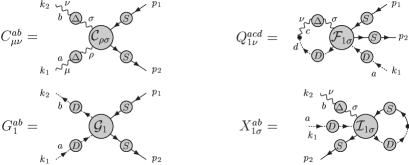
Figure 1: Diagrammatic representation of the Green’s function appearing in the STI of Eq.(4).

Thus, we arrive at the on-shell STI for ${\cal T}_{\mu\nu}^{ab}$

$$\mbox{}k_{1}^{\mu}{\cal T}_{\mu\nu}^{ab}={\cal S}^{ab}_{1\nu},$$

$$\mbox{}{\cal S}^{ab}_{1\nu}=igf^{bcd}{\cal Q}_{1\nu}^{acd}(k_{1},k_{2},p_{1},p_{2})D(k_{1})$$

$$\mbox{}-k_{2\nu}{\cal G}_{1}^{ab}(k_{1},k_{2},p_{1},p_{2})D(k_{1})D(k_{2}),$$ (5)

where we have defined $Q_{1\nu}^{acd}={\cal Q}_{1\nu}^{acd}D(k_{1})S(p_{1})S(p_{2})$.

In perturbation theory both ${\cal T}^{ab}_{\mu\nu}$ and ${\cal S}^{ab}_{1\nu}$ are given by Feynman diagrams, which can be separated into distinct classes, depending on their kinematic dependence and their geometrical properties. Graphs which do not contain information about the kinematical details of the incoming test-quarks are self-energy graphs, whereas those which display a dependence on the test quarks are vertex graphs. The former depend only on the variable $s$, whereas the latter on both $s$ and the mass $m$ of the test quarks; equivalently, we will refer to them as $s$-channel or $t$-channel graphs, respectively. In addition to the $s$-$t$ decomposition, Feynman diagrams can be separated into one-particle irreducible (1PI) and one-particle reducible (1PR) ones. The crucial point is that the action of the momenta $k_{1}^{\mu}$ or $k_{2}^{\nu}$ on ${\cal T}^{ab}_{\mu\nu}$ does not respect, in general, the original $s$-$t$ and 1PI-1PR separation furnished by the Feynman diagrams. In other words, even though Eq.(5) holds for the entire amplitude, it is not true for the individual sub-amplitudes, i.e.,

$$k_{1}^{\mu}\left[{\cal T}^{ab}_{\mu\nu}\right]_{x,{\rm{\scriptscriptstyle Y}}}\neq\left[{\cal S}^{ab}_{1\nu}\right]_{x,{\rm{\scriptscriptstyle Y}}},\quad x=s,t;\,\,\,{\rm Y=I,R},$$ (6)

where I (respectively R) indicates the one-particle irreducible (respectively reducible) parts of the amplitude involved. Evidently, whereas the characterization of graphs as propagator- and vertex-like is unambiguous in the absence of longitudinal momenta (e.g., in a scalar theory), their presence tends to mix propagator- and vertex-like graphs. Similarly, 1PR graphs are effectively converted into 1PI ones (the opposite cannot happen). The reason for the inequality of Eq.(6) are precisely the propagator-like terms, such as those encountered in the one- and two-loop calculations; they have the characteristic feature that, when depicted by means of Feynman diagrams contain unphysical vertices, i.e., vertices which do not exist in the original Lagrangian (Fig.2). All such diagrams cancel diagrammatically against each other.

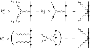
Figure 2: Diagrammatic representation of the tree-level inequality of Eq.(6)

In particular then, after the PT cancellations have been enforced, we find that the $t$-channel irreducible part satisfies the identity

$$\left[k_{1}^{\mu}{\cal T}^{ab}_{\mu\nu}\right]_{t,{\rm{\scriptscriptstyle I}}}^{{\scriptscriptstyle\rm PT}}\equiv\left[{\cal S}^{ab}_{1\nu}\right]_{t,{\rm{\scriptscriptstyle I}}}.$$ (7)

The non-trivial step for generalizing the PT to all orders is then the following: Instead of going through the arduous task of manipulating the left hand-side of Eq.(7) in order to determine the pinching parts and explicitly enforce their cancellation, use directly the right-hand side, which already contains the answer! Indeed, the right-hand side involves only conventional (ghost) Green’s functions, expressed in terms of normal Feynman rules, with no reference to unphysical vertices. Thus, its separation into propagator- and vertex-like graphs can be carried out unambiguously, since all possibility for mixing has been eliminated.

After these observations, we proceed to the PT construction to all orders. Once the effective Green’s functions have been derived, they will be compared to the corresponding Green’s functions obtained in the context of the Background Field Method Feynman gauge (BFMFG), in order to establish whether the known one- and two-loop correspondence persists to all orders; as we will see, this is indeed the case (for an extended list of related references see [8]).

To begin with, it is immediate to recognize that in the RFG box diagrams of arbitrary order $n$, to be denoted by $B^{[n]}$, coincide with the PT boxes ${\widehat{B}}^{[n]}$, since all three-gluon vertices are “internal”, i.e., they do not provide longitudinal momenta. Thus, they coincide with the BFMFG boxes, $\tilde{B}^{[n]}$, i.e., ${\widehat{B}}^{[n]}=B^{[n]}=\tilde{B}^{[n]}$ for every $n$.

We then continue with the construction of the one-particle irreducible PT gluon-quark–anti-quark vertex $\widehat{\Gamma}^{e}_{\alpha}$. We start from the corresponding vertex in the RFG, to be denoted by $\Gamma^{e}_{\alpha}$, and focus only on the class of vertex diagrams containing an external bare three-gluon vertex; we will denote this subset by $\Gamma^{e}_{\!A^{3},\alpha}$ [Fig.3(a)]. All other types of graphs contributing to $\Gamma^{e}_{\alpha}$ are inert as far as the PT procedure is concerned, because they do not furnish pinching momenta [7]. The next step is to carry out the vertex decomposition of Eq.(1) to the external three-gluon vertex $\Gamma^{eab,[0]}_{\alpha\mu\nu}$ appearing in $\Gamma^{e}_{\!A^{3},\alpha}$. This will result in the obvious separation $\Gamma^{e}_{\!A^{3},\alpha}=\Gamma^{{\rm F}\!,\,e}_{\!A^{3},\alpha}+\Gamma^{{\rm P}\!,\,e}_{\!A^{3},\alpha}$. The part $\Gamma^{{\rm F}\!,\,e}_{\!A^{3},\alpha}$ is also inert, and will be left untouched. Thus, the only quantity to be further manipulated is $\Gamma^{{\rm P}\!,\,e}_{\!A^{3},\alpha}$; it reads

$$\Gamma^{{\rm P\!,\,}e}_{\!A^{3},\alpha}\!\!=\!\!gf^{eba}\int\left[(k-q)^{\mu}g^{\nu}_{\alpha}+k^{\nu}g^{\mu}_{\alpha}\right]\left[{\cal T}_{\mu\nu}^{ab}\right]_{t,{\rm I}},$$ (8)

where $\int\equiv\mu^{2\varepsilon}\int d^{d}k/(2\pi)^{d}$, with $d=4-2\varepsilon$, and $\mu$ is the ’t Hooft mass. Following the discussion presented above, the pinching action amounts to the replacement $(-k+q)^{\mu}[{\cal T}_{\mu\nu}^{ab}]_{t,{\rm I}}\to[(-k+q)^{\mu}{\cal T}_{\mu\nu}^{ab}]_{t,{\rm I}}=\left[{\cal S}_{1\nu}^{ab}(-k+q,k)\right]_{t,{\rm I}}$ and similarly for the term coming from the momentum $k^{\nu}$, or, equivalently,

$$\Gamma^{{\rm P\!,\,}e}_{\!A^{3},\alpha}\rightarrow gf^{eba}\!\int\bigg{(}[{\cal S}_{2\alpha}^{ab}]_{t,{\rm I}}-[{\cal S}_{1\alpha}^{ab}]_{t,{\rm I}}\bigg{)}\!,$$ (9)

being ${\cal S}_{2\alpha}^{ab}$ the Bose symmetric of the ${\cal S}_{1\alpha}^{ab}$ term.

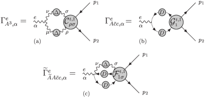
Figure 3: The Green’s functions identified in the construction of the all order PT vertex $\widehat{\Gamma}^{e}_{\alpha}$. (b) and (c) receive a contribution from similar terms with the ghost arrows reversed (not shown).

At this point the construction of the effective PT vertex $\widehat{\Gamma}^{e}_{\alpha}$ has been completed. The next important point is to study the connection between $\widehat{\Gamma}^{e}_{\alpha}$ and the gluon–quark–anti-quark vertex $\widetilde{\Gamma}^{e}_{\alpha}$ in the BFMFG. To begin with, all “inert” terms contained in the original $\Gamma^{e}_{\alpha}$ carry over to the same sub-groups of graphs obtained in the BFMFG; most notably, the $\Gamma^{{\rm F}\!,\,e}_{\!A^{3},\alpha}$ is precisely the $\Gamma^{e}_{\!\widetilde{A}A^{2},\alpha}$ part of $\widetilde{\Gamma}^{e}_{\alpha}$, where $\widetilde{A}$ is the background gluon. The only exception are the ghost-diagrams contributing to $\Gamma^{e}_{\alpha}$ [Fig.3(b)]; the latter do not coincide with the corresponding ghost contributions in the BFMFG. The important step is to recognize that the BFMFG ghost sector is provided precisely by combining the RFG ghosts with the right-hand side of Eq.(7). Specifically, one arrives at both the symmetric vertex $\widetilde{\Gamma}_{\widetilde{A}\bar{c}c}^{e}$, characteristic of the BFMFG, as well as at the background-gluon–gluon–ghost–anti-ghost vertex $\widetilde{\Gamma}_{\!\widetilde{A}A\bar{c}c}^{e}$, which is totally absent in the conventional formalism [Fig.3(c)]. Indeed, using Eq.(9), we find

$$\mbox{}\widetilde{\Gamma}^{e}_{\!\widetilde{A}\bar{c}c,\alpha}\!(q)\!\equiv\!\Gamma^{e}_{\bar{c}c,\alpha}(q)\!-\!gf^{eba}\!\!\!\int\!\!\!\left\{\!k_{\alpha}\!\left[{\cal G}_{1}^{ab}(-k+q,k)\!\right]_{t,{\rm I}}\right.$$

$$\mbox{}\left.-(k-q)_{\alpha}\left[{\cal G}_{2}^{ab}(-k+q,k)\right]_{t,{\rm I}}\right\}D(-k+q)D(k),$$

$$\mbox{}\widetilde{\Gamma}^{e}_{\!\widetilde{A}A\bar{c}c,\alpha}\!(q)\!\equiv\!ig^{2}\!f^{eba}\!\!\!\!\int\!\!\!\left\{\!f^{acd}\!\left[\!{\cal Q}_{2\alpha}^{cdb}(-k+q,k)\!\right]_{t,{\rm I}}\!\!D(k)\right.$$

$$\mbox{}\left.+f^{bcd}\left[{\cal Q}_{1\alpha}^{acd}(-k+q,k)\right]_{t,{\rm I}}D(-k+q)\right\}.$$ (10)

This last step concludes the proof that the equality $\widehat{\Gamma}^{e}_{\alpha}\equiv\widetilde{\Gamma}^{e}_{\alpha}$ between the PT and BFMFG vertex holds true to all orders. We emphasize that the sole ingredient in the above construction has been the STI of Eq.LABEL:(onshSTI); in particular, at no point have we employed a priori the BFM formalism. Instead, the special BFM ghost sector has arisen dynamically, once the PT rearrangement has taken place.

The final step is to construct the (all orders) PT gluon self-energy $\widehat{\Pi}^{ab}_{\mu\nu}$. Notice that at this point one would expect that it too coincides with the BFG gluon self-energy $\widetilde{\Pi}^{ab}_{\mu\nu}$, since both the boxes as well as the vertex do coincide with the corresponding quantities in BFG, and the $S$-matrix is unique. In fact this has been shown to be the case both through an inductive proof as well as by a direct construction [6].

In conclusion, we have shown that the use of the underlying BRST symmetry allows (trough the PT algorithm) for the construction of gauge independent and gauge invariant Green’s functions in QCD. It would be interesting to further explore the physical meaning of the $n$-point functions obtained [9], and establish possible connections with related formalisms.

Acknowledgments: This work has been supported by the CICYT Grants AEN-99/0692 and FPA-2002-00612.  J.P. thanks the organizers of QCD 03 for their hospitality and for providing a very pleasant and stimulating atmosphere.

References

- [1] A. A. Slavnov, Theor. Math. Phys. 10, 99 (1972) [Teor. Mat. Fiz. 10, 153 (1972)]; J. C. Taylor, Nucl. Phys. B 33, 436 (1971).
- [2] J. M. Cornwall, Phys. Rev. D 26, 1453 (1982).
- [3] J. M. Cornwall and J. Papavassiliou, Phys. Rev. D 40, 3474 (1989).
- [4] J. Papavassiliou and A. Pilaftsis, Phys. Rev. Lett. 75 (1995) 3060; Phys. Rev. D 53 (1996) 2128; Phys. Rev. D 54 (1996) 5315.
- [5] C. Becchi, A. Rouet and R. Stora, Annals Phys. 98, 287 (1976); I. V. Tyutin, Lebedev Institute Report, 75-39.
- [6] D. Binosi and J. Papavassiliou, Phys. Rev. D 66, 111901 (2002); arXiv:hep-ph/0209016; arXiv:hep-ph/0301096.
- [7] J. Papavassiliou, Phys. Rev. Lett. 84, 2782 (2000); Phys. Rev. D 62, 045006 (2000).
- [8] D. Binosi and J. Papavassiliou, Phys. Rev. D 66, 025024 (2002).
- [9] J. Bernabeu, J. Papavassiliou and J. Vidal, Phys. Rev. Lett. 89, 101802 (2002).