The SCET_II and factorization

Abstract

We reformulate the soft-collinear effective theory which includes the collinear quark and soft gluons. The quark form factor is used to prove that SCET_II reproduces the IR physics of the full theory. We give a factorization proof in deep inelastic lepton-hadron scattering by use of the position space formulation.

I Introduction

Perturbative QCD (pQCD) provides a powerful method to calculate the hard processes with large momentum transfers $Q\gg\Lambda_{\rm QCD}$ from the first principle CSS ; BL . The key ingredient of pQCD is factorization, which separates short-distance dynamics from the long-distance physics. Recently, an effective filed theory for soft and collinear particles were proposed in a series of studies B1 ; B2 ; B3 ; B4 ; B5 ; B6 . The proof of the factorization theorem in the soft-collinear effective theory (SCET) can be performed at the operator level which is much simpler than the diagrammatic analysis in pQCD. It also provides a new framework to study the resummation of Sudakov double-logs and the power corrections.

The SCET is divided into SCET_I and SCET_II according to the momentum of the collinear particles. It is convenient to use the light-cone coordinates $p^{\mu}=(p^{+},p^{-},p_{\bot})$ where $p^{+}=n_{-}\cdot p,~{}p^{-}=n_{+}\cdot p$ and $n_{+},~{}n_{-}$ are two light-like vectors which satisfy $n_{+}^{2}=n_{-}^{2}=0$ and $n_{+}\cdot n_{-}=2$. For the process where the off-shellness of the collinear particle $p_{c}^{2}\sim Q\Lambda_{\rm QCD}$, the soft particle belongs to ultrasoft mode. The momenta of the collinear and ultrasoft particles are scaled as $p_{c}\sim Q(\lambda^{2},1,\lambda)$ and $p_{us}\sim Q(\lambda^{2},\lambda^{2},\lambda^{2})$ where $\lambda=\sqrt{\Lambda_{\rm QCD}/Q}$. The theory of describing the collinear and ultrasoft fields is called SCET_I. For the processes where the off-shellness of the collinear particle $p_{c}^{2}\sim\Lambda_{\rm QCD}^{2}$, the soft particle belongs to soft mode. The momenta of the collinear and soft particles are scaled as $p_{c}\sim Q(\lambda^{2},1,\lambda)$ and $p_{s}\sim Q(\lambda,\lambda,\lambda)$ where $\lambda=\Lambda_{\rm QCD}/Q$. The SCET_II aims to describe the collinear and soft fields.

The construction of the SCET_II is considered more complicated than the SCET_I because the momentum of the collinear particle does not retain its scaling when a soft particle couples to it. A view about the SCET_II is that it can be considered as a low energy effective theory of SCET_I and is obtained from the the SCET_I by integrating out the ${\cal O}(\sqrt{Q\Lambda_{\rm QCD}})$ fluctuations. According to this view of point, in the leading order of $\lambda$, there is no coupling of soft to collinear particles in the SCET_II. However, the above arguments of excluding the interaction between the collinear and soft particles (in the leading order) are insufficient. Recalling that in the Heavy-Quark Effective Theory (HQET) Georgi , although the off-shellness of a heavy quark $p_{Q}^{2}=(m_{Q}v+k)^{2}\sim m_{Q}\Lambda_{\rm QCD}$ is at a large intermediate scale, the leading order HQET Lagrangian is given by the interaction of the heavy quark and soft gluons as ${\cal L}_{HQET}=\bar{h}_{v}iv\cdot D_{s}h_{v}$. The leading order interaction of the collinear quark and soft gluon had been proposed in the framework of the Large-Energy-Effective-Theory (LEET) DG . The LEET was criticized by lacking the collinear gluon degrees of freedom in the development of the SCET. Because the interactions of the collinear quark and soft gluon in the LEET is not contradict to any physical principle, another way of constructing the SCET_II can be done by adding the collinear gluon into the LEET. This is our proposal. The construction of the interactions of the collinear quark and soft gluons in the leading order at the Lagrangian level is more transparent and it is easier to be extended to higher orders.

We will study the quark form factor in the asymptotic limit in the SCET_II. First, we will show that the SCET_II reproduce the IR physics of QCD for the quark form factor at one-loop order. Then we use the SCET_II to give a factorized form for the quark form factor in the asymptotic limit. Another motivation of this study is to explore the proof of factorization by using the position space representation of SCET. In the position space representation, one can use the conventional definition of the universal non-perturbative quantities. As an example, we discuss the factorization proof in deep inelastic lepton-hadron scattering (DIS) process.

II The SCET_II Lagrangian

It is convenient to use the light-cone coordinates to study the processes which contain highly energetic light hadrons or jets. An arbitrary four-vector $p^{\mu}$ is written as

$$p^{\mu}=(p^{+},p^{-},p_{\bot})=n_{-}\cdot p\frac{n_{+}^{\mu}}{2}+n_{+}\cdot p\frac{n_{-}^{\mu}}{2}+p_{\bot}^{\mu},$$ (1)

where $n_{+}^{\mu}=(2,0,0_{\bot})$ and $n_{-}^{\mu}=(0,2,0_{\bot})$ are two light-like vectors which satisfy $n_{+}^{2}=n_{-}^{2}=0$, and $n_{+}\cdot n_{-}=2$. We discuss a case that all collinear particles move close to $n_{-}$ direction, i.e., the momentum $p^{-}\sim Q$ is large at first for the simplification of illustration. Other cases can be similarly obtained. A four-component Dirac field $\psi$ can be decomposed into two-component spinors $\xi$ and $\eta$ by

$$\psi=\xi+\eta,~{}~{}~{}~{}\xi\equiv P_{-}\psi=\frac{\hbox to0.0pt{\hskip 0.56917pt/\hss}{n}_{-}\hbox to0.0pt{\hskip 0.56917pt/\hss}{n}_{+}}{4}\psi,~{}~{}~{}~{}\eta\equiv P_{+}\psi=\frac{\hbox to0.0pt{\hskip 0.56917pt/\hss}{n}_{+}\hbox to0.0pt{\hskip 0.56917pt/\hss}{n}_{-}}{4}\psi.$$ (2)

with $\hbox to0.0pt{\hskip 0.56917pt/\hss}{n}_{-}\xi=\hbox to0.0pt{\hskip 0.56917pt/\hss}{n}_{+}\eta=0$. We will consider the effective theory for massless quarks because the mass of the light $u,d$ quarks are much smaller than the QCD confinement scale $\Lambda_{\rm QCD}$. The massless QCD Lagrangian ${\cal L}=\bar{\psi}~{}i\hbox to0.0pt{\hskip 2.27626pt/\hss}{D}\psi$ is

$${\cal L}=\bar{\xi}~{}in_{-}\cdot D\frac{\hbox to0.0pt{\hskip 0.56917pt/\hss}{n}_{+}}{2}~{}\xi+\bar{\eta}~{}in_{+}\cdot D\frac{\hbox to0.0pt{\hskip 0.56917pt/\hss}{n}_{-}}{2}~{}\eta+\bar{\xi}~{}i\hbox to0.0pt{\hskip 2.27626pt/\hss}{D}_{\bot}\eta+\bar{\eta}~{}i\hbox to0.0pt{\hskip 2.27626pt/\hss}{D}_{\bot}\xi.$$ (3)

where $D_{\mu}=\partial_{\mu}-igA_{\mu}=\partial_{\mu}-igT^{a}A_{\mu}^{a}$.

As we have discussed in the Introduction, the SCET_II describes the degrees of freedom of the collinear and soft fields. The momenta for the collinear and soft particles are scaled as $p_{c}\sim Q(\lambda^{2},1,\lambda)$ and $p_{s}\sim Q(\lambda,\lambda,\lambda)$ where $\lambda=\Lambda_{\rm QCD}/Q$. The power counting for the relevant fields can be found in BCDF : the collinear quark field $\xi\sim\lambda$; the collinear gluon field: $A_{c}^{\mu}\sim(\lambda^{2},1,\lambda)$; the soft quark field: $q_{s}\sim\lambda^{3/2}$; the soft gluon field: $A_{s}\sim\lambda$.

Now, we follow the construction of the LEET given in DG ; CYOPR and then transform it into the position space representation. After the interactions with the soft gluon, the momentum of the collinear quark is changed into $p=p_{c}+k$ where $k\sim Q(\lambda,\lambda,\lambda)$ is the residual momentum carried by the soft gluons. Thus, the scaling of the integral element is $d^{4}x\sim\frac{1}{d^{4}p}\sim\lambda^{-3}$ rather than $\lambda^{-4}$. Analogous to the HQET, we remove the large momentum component $p^{-}$ by redefining the collinear quark field as $\psi(x)=e^{-i\frac{(n_{+}\cdot p)}{2}n_{-}\cdot x}[\xi_{p^{-}}(x)+\eta_{p^{-}}(x)]$. After integrating out the small-component field $\eta_{p^{-}}(x)$, one obtain the effective Lagrangian for the interaction of collinear quark with the soft gluons as

$${\cal L}_{c-s}=\sum_{p^{-}}\bar{\xi}_{p^{-}}\left[~{}in_{-}\cdot D_{s}+i\hbox to0.0pt{\hskip 2.27626pt/\hss}{D}_{s\bot}\frac{1}{~{}n_{+}\cdot p+in_{+}\cdot D_{s}}~{}i\hbox to0.0pt{\hskip 2.27626pt/\hss}{D}_{s\bot}~{}\right]\frac{\hbox to0.0pt{\hskip 0.56917pt/\hss}{n}_{+}}{2}~{}\xi_{p^{-}}.$$ (4)

where $D_{s}=\partial_{s}-igA_{s}$ and $\partial_{s}$ scales as a soft momentum. The lowest order effective Lagrangian for the collinear quark and soft gluon interaction is

$${\cal L}_{c-s}^{(0)}=\sum_{p^{-}}\bar{\xi}_{p^{-}}~{}in_{-}\cdot D_{s}\frac{\hbox to0.0pt{\hskip 0.56917pt/\hss}{n}_{+}}{2}~{}\xi_{p^{-}}.$$ (5)

Eq. (5) is the LEET Lagrange proposed in DG . Eq. (4) also provides the higher order terms which is given in the second term of it. Since only the $n_{-}\cdot A_{s}$ gluons contribute at the lowest order, one can write $\xi_{p^{-}}(x)$ field in another way as

$$\xi_{p^{-}}(x)=W_{s}(x)~{}\xi^{0}_{p^{-}}(x),~{}~{}~{}~{}~{}W_{s}(x)={\rm P~{}exp}\left(ig\int_{-\infty}^{0}dt~{}n_{-}\cdot A_{s}(x+tn_{-})\right).$$ (6)

The field $\xi^{0}$ is a quark field without coupling to the soft gluons. The ${\rm P}$ in the soft Wilson line $W_{s}$ denotes path-ordering defined such that the the gluon fields stand to the left for larger values of parameter $t$.

The previous obstruction of constructing the leading order interaction of the collinear quark with soft gluons in the SCET_II lies in the different scaling of momenta $p_{c}$ and $p_{c}+k_{s}$. In the above analysis, the main assumption we use is that $p^{-}$ is the largest momentum component. The $\xi_{p^{-}}(x)$ field is a collinear field rather than a soft field like the heavy quark field $h_{v}(x)$. This can be seen from Eq. (6). The off-shellness of $p_{c}+k_{s}$ does not invalidate our assumption. It is the superselection rule of momentum component $p^{-}$ (the energy of the collinear particle) that permits us to write down the lowest order effective interaction of Eq. (5) at the Lagrangian level. Other interaction, such as the collinear gluon coupling to the heavy quark can not can not been done in this way. From another point of view, the information of the off-shellness cause by $p^{-}k^{+}$ can be included in the soft Wilson line, so the construction of the leading order effective Lagrange is equivalent to the use of the soft Wilson line. The advantage of our proposal is that it permits us to write down not only the leading order term but also the higher order terms systematically.

Transforming the above analysis into the position space formulation can be done straightforwardly by using the correspondence rule $p\to i\partial$. The index of $p^{-}$ in the field $\xi_{p^{-}}$ can be dropped. We also include the collinear gluon in the effective theory. The procedure is done by integrating out the $\eta$ field and then insert the solution into Eq. (3) as in BCDF , we obtain an effective Lagrangian for SECT_II as

$${\cal L}_{\rm SCET_{II}}=\bar{\xi}\left[~{}in_{-}\cdot D+i\hbox to0.0pt{\hskip 2.27626pt/\hss}{D}_{\bot}\frac{1}{~{}in_{+}\cdot D}~{}i\hbox to0.0pt{\hskip 2.27626pt/\hss}{D}_{\bot}\right]\frac{\hbox to0.0pt{\hskip 0.56917pt/\hss}{n}_{+}}{2}~{}\xi.$$ (7)

where the covariant derivative is defined by $D=\partial-igA_{c}-igA_{s}$. The Eq. (7) contains the interaction of the collinear quark with collinear gluon

$${\cal L}_{c-c}=\bar{\xi}\left[~{}in_{-}\cdot D_{c}+i\hbox to0.0pt{\hskip 2.27626pt/\hss}{D}_{c\bot}\frac{1}{~{}in_{+}\cdot D_{c}}~{}i\hbox to0.0pt{\hskip 2.27626pt/\hss}{D}_{c\bot}\right]\frac{\hbox to0.0pt{\hskip 0.56917pt/\hss}{n}_{+}}{2}~{}\xi.$$ (8)

The interaction of the collinear quark with soft gluon is given in Eq. (4). The new interaction terms of the collinear quark, collinear gluon and soft gluon appear, such as ${\cal L}_{s-c}=\bar{\xi}\left[i\hbox to0.0pt{\hskip 2.27626pt/\hss}{D}_{s\bot}\frac{1}{~{}in_{+}\cdot D_{c}}~{}i\hbox to0.0pt{\hskip 2.27626pt/\hss}{D}_{c\bot}+i\hbox to0.0pt{\hskip 2.27626pt/\hss}{D}_{c\bot}\frac{1}{~{}in_{+}\cdot D_{c}}~{}i\hbox to0.0pt{\hskip 2.27626pt/\hss}{D}_{s\bot}\right]\frac{\hbox to0.0pt{\hskip 0.56917pt/\hss}{n}_{+}}{2}~{}\xi$ which are $\lambda$ order corrections. One must keep in mind that the scaling of the integral element $d^{4}x$ is $\lambda^{4}$ for the collinear-collinear interaction and $\lambda^{3}$ for collinear-soft interaction. The full SCET_II should contain the soft quarks as well. Some discussions about this part can be found in HN . We will not consider it in this study.

One can define the collinear Wilson line $W_{c}$ in a similar way as the soft Wilson line by

$$W_{c}(x)={\rm P~{}exp}\left(ig\int_{-\infty}^{0}dt~{}n_{+}\cdot A_{c}(x+tn_{+})\right).$$ (9)

We will use the collinear Wilson line in the proof of factorization below.

The SCET contains rich symmetry structures. Except the symmetries which had been studied largely in the literatures, we discuss a new symmetry: scale symmetry. However, this symmetry is not rigorous but approximate. It is broken by the renormalization effect and quark mass. In the SCET_II, the light quark mass is approximated to zero. In most high energy hard processes, the broken of the scale symmetry is caused by the perturbative corrections occurred at the scale of ${\cal O}(Q)$ which is suppressed by the coupling constant $\alpha_{s}(Q)$. If neglecting the perturbative corrections, the scale symmetry can be a useful guide. For the SCET, the effective Lagrangian at tree level is scale invariant. The scale transformation is defined as

$$x_{\mu}\to s^{-1}x_{\mu},~{}~{}~{}~{}~{}\partial_{\mu}\to s~{}\partial_{\mu},~{}~{}~{}~{}~{}\xi\to s^{3/2}\xi,~{}~{}~{}~{}~{}A_{\mu}\to sA_{\mu}.$$ (10)

It is easy to check that the action $\int d^{4}x{\cal L}_{\rm SCET_{II}}$ is invariant under the above scale transformation.

III The quark form factor

The quark form factor in the asymptotic limit provides a simple example to discuss the Sudakov resummation and factorization Collins . We use this example to check whether SCET_II reproduces all the IR physics of QCD. We consider a form factor given by $\langle B|\bar{\psi}_{B}\gamma_{\mu}\psi_{A}|A\rangle=\bar{u}_{B}\gamma_{\mu}u_{A}F$ in the full QCD. The current is electromagnetic. The process is that an initial energetic quark A absorbs a highly off-shell photon and transforms into a final energetic quark B in the opposite direction. We choose the transition form factor rather than the annihilation form factor in order to avoid the unimportant imaginary part. We study the case that the collinear quarks are both on-shell. The momenta of quarks A and B are chosen as $p_{A}=(Q,0,0_{\bot}),~{}p_{B}=(0,Q,0_{\bot})$ and $q^{2}=(p_{B}-p_{A})^{2}=-Q^{2}$ where $Q$ is a large energy scale.

The one-loop order QCD corrections to the quark transition form factor contain the quark self-energy and the vertex corrections. The light quark self-energy corrections are same in the full theory and the effective theory B2 . We will not consider them below. The one-loop vertex correction depicted in Fig. 1 contains the ultraviolet (UV) divergences as well as the collinear and soft divergences. The collinear divergence appears when the virtual gluon becomes collinear to quark A or B. One may use the quark mass and a fictitious mass for gluon field to regulate the IR singularities. The problem of this regularization method is that it is insufficient to regulate all the singularities in the effective theory. We will use the regularization method proposed in BDS because it simplifies the calculation. The IR regulator is given by adding new terms in the Lagrangian:

$${\cal L}_{reg}=-\frac{\delta}{2}A_{+\mu}(in_{-}\cdot\partial)A^{\mu}_{+}-\frac{\delta}{2}A_{s\mu}(in_{-}\cdot\partial)A^{\mu}_{s}+(+\leftrightarrow-).$$ (11)

where $A_{+}$ represents the gluon collinear to the A quark. The appearance of the additional terms $(+\leftrightarrow-)$ is because there are two collinear quarks with different directions in our process.

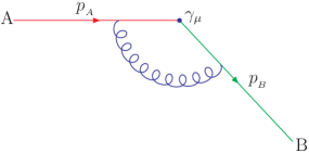
Figure 1: The one-loop vertex correction to the quark form factor.

We use the dimensional regularization to regulate the UV divergences and perform the calculation in $d=4-2\epsilon$ dimension. The one-loop vertex correction in the full theory plotted in Fig. 1 is given by

$$I_{full}=-ig_{s}^{2}C_{F}\mu^{\prime 2\epsilon}\int\frac{d^{d}k}{(2\pi)^{d}}\frac{\gamma_{\rho}(\hbox to0.0pt{\hskip 0.56917pt/\hss}{k}+\hbox to0.0pt{\hskip 0.56917pt/\hss}{p}_{B})\gamma_{\mu}(\hbox to0.0pt{\hskip 0.56917pt/\hss}{k}+\hbox to0.0pt{\hskip 0.56917pt/\hss}{p}_{A})\gamma^{\rho}}{[(k+p_{A})^{2}+i\epsilon][(k+p_{B})^{2}+i\epsilon][k^{2}-\delta(n_{+}+n_{-})\cdot k+i\epsilon]}.$$ (12)

The calculation of the above integral can be done in the conventional way and the full theory result is

$$I_{full}=\frac{\alpha_{s}}{4\pi}C_{F}\gamma_{\mu}\left[\frac{1}{\epsilon}+{\rm ln}\frac{\mu^{2}}{Q^{2}}-\frac{1}{2}{\rm ln}^{2}\frac{Q^{2}}{\delta^{2}}+2{\rm ln}\frac{Q^{2}}{\delta^{2}}-\frac{\pi^{2}}{3}\right]$$ (13)

where $\mu^{2}=4\pi\mu^{\prime 2}{\rm e}^{-\gamma_{E}\epsilon}$ and $\gamma_{E}$ is the Euler constant.

Maybe the best way to check that SCET reproduces the IR physics of the full QCD is performed by using the method of regions BS . The idea is expanding the integrand $I$ in the momentum regions which give contributions in dimensional regularization. In the quark form factor, the non-vanishing contributions come from the hard region where the momentum of the virtual gluon $k\sim(1,1,1)$, collinear-A region where $k\sim(1,\lambda^{2},\lambda)$, collinear-B region where $k\sim(\lambda^{2},1,\lambda)$ and soft region where $k\sim(\lambda,\lambda,\lambda)$.

For the hard region, we can set $\delta=0$. The hard region contribution is

$$I_{h} = -ig_{s}^{2}C_{F}\mu^{\prime 2\epsilon}\int\frac{d^{d}k}{(2\pi)^{d}}\frac{\gamma_{\rho}(\hbox to0.0pt{\hskip 0.56917pt/\hss}{k}+\hbox to0.0pt{\hskip 0.56917pt/\hss}{p}_{B})\gamma_{\mu}(\hbox to0.0pt{\hskip 0.56917pt/\hss}{k}+\hbox to0.0pt{\hskip 0.56917pt/\hss}{p}_{A})\gamma^{\rho}}{[k^{2}+2p_{A}\cdot k+i\epsilon][k^{2}+2p_{B}\cdot k+i\epsilon][k^{2}+i\epsilon]}$$ (14)

$$= \frac{\alpha_{s}}{4\pi}C_{F}\gamma_{\mu}\left[-\frac{2}{\epsilon^{2}}-\frac{3+2{\rm ln}\frac{\mu^{2}}{Q^{2}}}{\epsilon}-{\rm ln}^{2}\frac{\mu^{2}}{Q^{2}}-3{\rm ln}\frac{\mu^{2}}{Q^{2}}-8+\frac{\pi^{2}}{6}\right]$$

The collinear-A region comes from the contribution where the momentum $k$ is parallel to $p_{A}$. We make a transformation $k\to-k$ in Eq. (12). In this region, $\frac{\gamma_{\rho}(\hbox to0.0pt{\hskip 0.56917pt/\hss}{p}_{B}-\hbox to0.0pt{\hskip 0.56917pt/\hss}{k})}{k^{2}-2p_{B}\cdot k+i\epsilon}\to\frac{-n_{-\rho}}{n_{-}\cdot k}$. The collinear-A region contribution is

$$I_{A} = -ig_{s}^{2}C_{F}\mu^{\prime 2\epsilon}\int\frac{d^{d}k}{(2\pi)^{d}}\frac{-n_{-\rho}\gamma_{\mu}(\hbox to0.0pt{\hskip 0.56917pt/\hss}{p}_{A}-\hbox to0.0pt{\hskip 0.56917pt/\hss}{k})\gamma^{\rho}}{[k^{2}-2p_{A}\cdot k+i\epsilon]~{}(n_{-}\cdot k)~{}[k^{2}-\delta(n_{-}\cdot k)+i\epsilon]}$$ (15)

$$= \frac{\alpha_{s}}{4\pi}C_{F}\gamma_{\mu}\left[\frac{2}{\epsilon^{2}}+\frac{2+2{\rm ln}\frac{\mu^{2}}{Q\delta}}{\epsilon}+{\rm ln}^{2}\frac{\mu^{2}}{Q\delta}+2{\rm ln}\frac{\mu^{2}}{Q\delta}+4-\frac{\pi^{2}}{6}\right]$$

The above calculation is performed by the contour integration.

The collinear-B region contribution can be obtained from $I_{A}$ by $-\to+$ and $A\to B$. Since the final result of $I_{A}$ does not depend on the changes, the collinear-B region contribution is the same as $I_{A}$. Thus,

$$I_{B} = -ig_{s}^{2}C_{F}\mu^{\prime 2\epsilon}\int\frac{d^{d}k}{(2\pi)^{d}}\frac{\gamma_{\rho}(\hbox to0.0pt{\hskip 0.56917pt/\hss}{p}_{B}-\hbox to0.0pt{\hskip 0.56917pt/\hss}{k})\gamma_{\mu}(-n_{+}^{\rho})}{[k^{2}-2p_{B}\cdot k+i\epsilon]~{}(n_{+}\cdot k)~{}[k^{2}-\delta(n_{+}\cdot k)+i\epsilon]}$$ (16)

$$= \frac{\alpha_{s}}{4\pi}C_{F}\gamma_{\mu}\left[\frac{2}{\epsilon^{2}}+\frac{2+2{\rm ln}\frac{\mu^{2}}{Q\delta}}{\epsilon}+{\rm ln}^{2}\frac{\mu^{2}}{Q\delta}+2{\rm ln}\frac{\mu^{2}}{Q\delta}+4-\frac{\pi^{2}}{6}\right]$$

The soft region contribution is

$$I_{s} = -ig_{s}^{2}C_{F}\mu^{\prime 2\epsilon}\int\frac{d^{d}k}{(2\pi)^{d}}\frac{n_{-\rho}\gamma_{\mu}n_{+}^{\rho}}{[n_{-}\cdot k+i\epsilon][n_{+}\cdot k+i\epsilon][k^{2}-\delta(n_{+}+n_{-})\cdot k+i\epsilon]}$$ (17)

$$= \frac{\alpha_{s}}{4\pi}C_{F}\gamma_{\mu}\left[-\frac{2}{\epsilon^{2}}-\frac{2{\rm ln}\frac{\mu^{2}}{\delta^{2}}}{\epsilon}-{\rm ln}^{2}\frac{\mu^{2}}{\delta^{2}}-\frac{\pi^{2}}{6}\right]$$

The detailed calculation of the above results and the summation of the Sudakov double-logs will be given elsewhere.

The contributions from the collinear-A, collinear-B and soft regions are infrared physics. They also constitute the results in the SECT_II exactly. It can be checked that $I_{full}=I_{h}+I_{A}+I_{B}+I_{s}$. Thus, the IR physics of the quark form factor is reproduced in the SCET_II and the non-IR physics (it refers to the perturbative part in pQCD) is contained in the hard region contribution.

After the proof that SCET_II reproduces the IR physics of the quark form factor in the full theory, we can use the effective theory to give a factorization form. The advantage of using the SCET to study factorization is that we can use the operator language rather than diagram analysis and the proof to all orders can be done simply. The light-light current in the full QCD is: $\bar{\psi}_{B}\gamma_{\mu}\psi_{A}$; in the SCET_II, the current operator becomes as

$$\bar{\xi}_{n_{-}}W_{c}(n_{-})\gamma_{\mu}W_{c}^{\dagger}(n_{+})\xi_{n_{+}}W_{s}^{\dagger}(n_{-})W_{s}(n_{+})$$ (18)

where $\xi_{n_{-}}$ and $W_{c}(n_{-})$ represents the collinear field and collinear Wilson line along the $n_{-}$ direction. Similar definitions for the other operators are implied.

The factorized form for the quark form factor is

$$F=H\times J_{A}\times J_{B}\times S$$ (19)

where $J_{A}\equiv\langle 0|W_{c}^{\dagger}(n_{+})\xi_{n_{+}}|A\rangle$, $J_{B}\equiv\langle B|\bar{\xi}_{n_{-}}W_{c}(n_{-})|0\rangle$ and $S\equiv\langle 0|W_{s}^{\dagger}(n_{-})W_{s}(n_{+})|0\rangle$. Our definition of the jet-like and soft functions are different from that of Collins . The author in Collins may adopt a momentum subtraction to suppress the non-analytic terms in the integral of a momentum region in order to avoid the double counting. In the method of regions, these non-analytic terms cancel in the sum of the integrals for different momentum regions.

IV The factorziation in DIS

The factorization is the foundation of pQCD but to prove it is usually difficult. The deep inelastic lepton-hadron scattering (DIS) plays a central role in understanding the factorization in pQCD. In CSS , the diagrammatic analysis is used to prove the factorization to all orders of coupling constant $\alpha_{s}$ and leading order in $\lambda$ (or say $\Lambda_{\rm QCD}/Q$). The method of regions in BS may be also viewed as the diagrammatic analysis but a refined version which permits the analysis to higher orders in $\lambda$. As we have discussed in the quark form factor, the contributions of different regions (except for the hard region) are corresponding parts in the SCET. After we have checked that SCET produces all the IR physics of the full theory, we can use the operator language in SCET in place of the diagrammatic analysis to simplify the all-orders proof of factorization.

The study of the factorization in DIS in the framework of SCET has been given in B6 . There is a view that the effective theory used is SCET_I for the inclusive processes and SCET_II for the exclusive processes. In B6 , the authors apply the SCET_I to study the inclusive DIS process. This view is not rigorous. Which SECT theory is used as the final effective theory of a process depends on the momentum of collinear particle. In DIS, the proton and the collinear quark inside the proton have the virtuality of order of $\Lambda_{\rm QCD}$, so the correct theory needed is SCET_II rather than SCET_I. The analysis of B6 used a hybrid position-momentum space representation in which a definition of the parton distribution functions in the momentum space is introduced. We will use the position space representation developed in BCDF and the SCET_II to study the factorization in DIS. We can use the familiar definition of the parton distribution functions in the position space. We think our formalisms are more transparent and simpler than that in the hybrid position-momentum representation.

We consider the DIS process $e(k)+H(p)\to e(k^{\prime})+X$. The kinematical variable are defined as $q^{2}=-Q^{2}$ and $x=\frac{Q^{2}}{2p\cdot q}$ with $q=k^{\prime}-k$ and $p,m_{H}$ are the momentum and mass of the initial hadron. We are interested in the region that $Q\gg\Lambda_{\rm QCD}$ and $x$ is fixed but not small. We choose the frame so that $p^{\mu}=(0,\frac{Q}{x},0_{\bot})$ and $q^{\mu}=(Q,0,q_{\bot})$ with $q_{\bot}^{2}=Q^{2}$. Note that our choice of frame is not same as that in B6 .

The hadronic tensor of the DIS cross section is determined by

$$W_{\mu\nu}=\left(-g_{\mu\nu}+\frac{q_{\mu}q_{\nu}}{q^{2}}\right)F_{1}(x,Q^{2})+\frac{(p_{\mu}+\frac{q_{\mu}}{2x})(p_{\nu}+\frac{q_{\nu}}{2x})}{p\cdot q}F_{2}(x,Q^{2})$$ (20)

The $F_{1,2}$ are the standard structure functions. The hadronic tensor $W_{\mu\nu}$ is related to the forward scattering amplitude by

$$W_{\mu\nu}=\frac{1}{2\pi}\frac{1}{2}\sum_{\rm spin}\int d^{4}y~{}e^{iq\cdot y}\langle H|T[j_{\mu}(y)j_{\nu}(0)]|H\rangle$$ (21)

where $j_{\mu}$ is the electromagnetic current. In the discussions below, we will not write the spin average $\frac{1}{2}\sum_{\rm spin}$ for simplification. One can obtain the structure functions through the projecting of hadronic tensor by

$$n_{+}^{\mu}n_{+}^{\nu}W_{\mu\nu}=\frac{2}{x}F_{2},~{}~{}~{}~{}~{}~{}n_{-}^{\mu}n_{-}^{\nu}W_{\mu\nu}=\frac{1}{2x}F_{2}-F_{1}.$$ (22)

In the quark form factor, the leading contributions come from the hard, collinear and soft regions. For DIS, the soft divergences are cancelled due to the unitarity of Wilson line $W_{s}^{\dagger}(n_{-})W_{s}(n_{-})$. The collinear quarks are moving in the same direction in DIS which is different from the case in the quark form factor. So, there is no soft factor appeared in the factorization form in leading order. Physically, the cancellation of soft divergences is the result of summing over all final states.

Now, we consider the operator product $T[j_{\mu}(y)j_{\nu}(0)]$. This product is light-cone dominated, i.e., $0\leq y^{2}\leq\frac{\rm const.}{Q^{2}}$. We can not apply the conventional short distance operator-product-expansion Wilson to disentangle short-distance from long-distance dynamics. The light cone expansion was proposed to study the light-cone dominated processes. In SCET, one can use the SCET operators to expand the the operator product. We have shown that the SCET_II reproduces the IR physics of the full theory in the quark form factor. We expect that this conclusion can be applied in DIS. Thus, we can expand the operator product $T[j_{\mu}(y)j_{\nu}(0)]$ in terms of the SCET operators. Take $n_{+}^{\mu}n_{+}^{\nu}T[j_{\mu}(y)j_{\nu}(0)]$ as an example of illustration

$$n_{+}^{\mu}n_{+}^{\nu}T[j_{\mu}(y)j_{\nu}(0)]\longrightarrow\sum_{i}C_{i}(y)O_{i}(yn_{+}).$$ (23)

where $O_{i}$ are operators in SCET and $yn_{+}\equiv(n_{-}\cdot y)\frac{n_{+}}{2}$. In leading order of $\lambda$, the gauge invariant SCET operators which contain collinear quark and collinear gluon for DIS are given by

$$O_{i}^{q}=(\bar{\xi}W_{c})(yn_{+})\frac{\hbox to0.0pt{\hskip 0.56917pt/\hss}{n}_{+}}{2}W_{c}^{\dagger}\xi(0),~{}~{}~{}~{}~{}~{}O_{i}^{g}=\sum_{j=1}^{2}(F^{+j}W_{c})(yn_{+})W_{c}^{\dagger}F^{+}_{~{}j}(0).$$ (24)

where $F^{ij}$ is the gluon field strength operator. The appearance of the gluon operator starts from $\alpha_{s}$ order. The appearance of bilocal operators is the summation of infinite local operators of leading order (order $\lambda^{2}$). The physical interpretation is that the intermediate quark in the operator product can emit (or absorbs) a large number of collinear gluons in leading order. The Wilson coefficients $C_{i}$ in Eq. (23) are infrared finite because it is obtained from the matching from the full QCD onto the SCET_II. The Wilson coefficients contain the contribution from the hard region only and is insensitive to the IR physics in principle.

According to CSS , the hadronic matrix elements of the bilocal operator are defined by

$$\langle H(p)|\bar{\xi}(yn_{+})\frac{\hbox to0.0pt{\hskip 0.56917pt/\hss}{n}_{+}}{2}{\cal P}\xi(0)|H(p)\rangle = 2(n_{+}\cdot p)\int d\zeta~{}e^{i\zeta p^{-}y^{+}}f_{q/H}(\zeta),$$

$$\langle H(p)|F^{+j}(yn_{+}){\cal P}F^{+}_{~{}j}(0)|H(p)\rangle = \zeta(n_{+}\cdot p)^{2}\int d\zeta~{}e^{i\zeta p^{-}y^{+}}f_{g/H}(\zeta).$$ (25)

where ${\cal P}=W_{c}(yn_{+})W_{c}^{\dagger}(0)$ is the ordered exponential. $f_{q(g)/H}$ are parton distribution function for quarks or gluons. The variable $\zeta$ is the light-cone momentum fraction.

Introduce short-distance Wilsion coefficients in momentum space $\tilde{C}_{i}(\zeta,x,Q)$ through the Fourier transformation by

$$\tilde{C}_{i}(\zeta,x,Q)=\int d^{4}y~{}e^{i\left(q+\zeta(p\cdot n_{+})n_{-}\right)\cdot y}C_{i}(y)$$ (26)

Inserting Eqs. (23, 24, IV, 26) back into Eqs. (20, 21, 22), we obtain a convolution factorization formula for the structure functions

$$F_{1,2}(x,Q^{2})=\sum_{a}\int_{x}^{1}d\zeta~{}f_{a/H}(\zeta,\mu)H_{1,2}^{a}(\zeta,x,Q/\mu)$$ (27)

where $a$ represents quark or gluon and the hard scattering kernel $H_{1,2}^{a}(\zeta,x,Q/\mu)$ differs from $\tilde{C}_{i}(\zeta,x,Q/\mu)$ by constant factors. The factorization formula is a convolution form because both the parton distribution functions and the Wilson coefficients depend on $\zeta$. Thus, we proved that the structure functions can be factorized into a convolution of short-distant and long-distant parts.

V Discussions and conclusions

The study of the hard QCD processes has been a long history. The development of soft-collinear effective theory may make these processes more understandable. In this study, we reformulated the SCET_II along the line of the LEET. We give the leading order interaction of the collinear quark with soft gluons at the Lagrangian level. The higher order terms can be obtained from the effective Lagrangian. In our approach, the differences between SCET_II and the SCET_I are less than the previous studies. According to this view, most of the results in SCET_I may be applied into the SCET_II. But one keep in mind that the power counting of the soft-collinear interaction in SCET_II are different from the ultrasoft-collinear part in SCET_I. The more detailed study about this is necessary.

The quark form factor is used as an example to prove that SCET_II does reproduce all the IR physics of the full QCD. We studied the factorization of the quark form factor and DIS in SCET_II. Obvious, our proof is not full, but it contains the main ingredients. Although which representation is more convenient is not easy to evaluate, the position space representation is more simple and intuitive in the proof of factorization in our opinion. The SCET also provide a new framework to study the processes where the conventional operator-product-expansion is not applicable.

Although SCET has been studied in some literatures, we feel that the construction of SCET_II and its application into the processes where soft gluon does not cancel is still a difficult task. The study of exclusive B decays and other high energy processes such as diffractive scattering require better understanding of the SCET_II.

References

- (1) J.C. Collins, D.E. Soper and G. Sterman, in , ed. A.H. Mueller (World Scientific, Singapore, 1989), p1-91, and the references therein.
- (2) S.J. Brodsky and G.P. Lepage, in , ed. A.H. Mueller (World Scientific, Singapore, 1989), p93-240, and the references therein.
- (3) C.W. Bauer, S. Fleming and M.E. Luke, Phys. Rev. D63, 014006 (2001).
- (4) C.W. Bauer, S. Fleming, D. Pirjol and I.W. Stewart, Phys. Rev. D63, 114020 (2001).
- (5) C.W. Bauer and I.W. Stewart Phys. Lett. B 516, 134 (2001).
- (6) C.W Bauer, D. Pirjol and I.W. Stewart, Phys. Rev. Lett. 87, 201806 (2001).
- (7) C.W Bauer, D. Pirjol and I.W. Stewart, Phys. Rev. D65, 054022 (2002).
- (8) C.W. Bauer, S. Fleming, D. Pirjol, I.Z. Rothstein and I.W. Stewart, Phys. Rev. D66, 014017 2002.
- (9) H. Georgi, Phys. Lett. B 240, 447 (1990).
- (10) M.J. Dugan and B. Grinstein, Phys. Lett. B 255, 583 (1991).
- (11) M. Beneke, A.P. Chapovsky, M. Diehl and T. Feldmann, Nucl. Phys. B 643, 431 (2002).
- (12) J. Charles, A.L. Yaouanc, L. Oliver, O. Pene and J.C. Raynal, Phys. Rev. D60, 014001 1999.
- (13) R.J. Hill and Matthias Neubert, Nucl. Phys. B 657, 229 (2003).
- (14) J.C. Collins, D.E. Soper and G. Sterman, in , ed. A.H. Mueller (World Scientific, Singapore, 1989), p573-614.
- (15) C.W. Bauer, M.P. Dorsten and M. P. Salem, arXiv: hep-ph/0312302.
- (16) M. Beneke and V.A. Smirnov, Nucl. Phys. B 522, 321 (1998).
- (17) K.G. Wilson, Phys. Rev. D179, 1499 (1969).