Bosonic Quartic Couplings at LHC

Abstract

We analyze the potential of the CERN Large Hadron Collider (LHC) to study anomalous quartic vector–boson interactions $ZZ\gamma\gamma$, $ZZZ\gamma$, $W^{+}W^{-}\gamma\gamma$, and $W^{+}W^{-}Z\gamma$ through the weak boson fusion processes $qq\to qq\gamma\gamma$ and $qq\to qq\gamma Z(\to\ell^{+}\ell^{-})$ with $\ell=e$ or $\mu$. After a careful study of the backgrounds and how to extract them from the data, we show that the process $pp\to jj\gamma l^{+}l^{-}$ is potentially the most sensitive to deviations from the Standard Model, improving the sensitivity to anomalous couplings by up to a factor $10^{4}$ ($10^{2}$) with respect to the present direct (indirect) limits.

I Introduction

Within the framework of the Standard Model (SM), the structure of the trilinear and quartic vector–boson couplings is completely determined by the $SU(2)_{L}\times U(1)_{Y}$ gauge symmetry. The study of these interactions can either lead to an additional confirmation of the model or give some hint on the existence of new phenomena at a higher scale anomalous . The triple gauge–boson couplings have been probed at the Tevatron teva and LEP lep ; ewwg through the production of vector–boson pairs, however, we have only started to study directly the quartic gauge–boson couplings  quarticnow ; ewwg ; Belanger:1999aw ; stir1 . If any deviation from the SM predictions is observed, independent tests of the triple and quartic gauge–boson couplings can give important information on the type of New Physics (NP) responsible for the deviations. For example, the exchange of heavy bosons can generate a tree level contribution to four gauge–boson couplings while its effect in the triple–gauge vertex would only appear at one one–loop, and consequently be suppressed with respect to the quartic one. Further information on the NP dynamics can also be provided by determining whether NP reveals itself in the form of anomalous four-gauge couplings involving only weak gauge bosons or in those involving photons or in both.

At present the scarce experimental information on quartic anomalous couplings arises from the processes $e^{+}e^{-}\rightarrow W^{+}W^{-}\gamma$, $Z\gamma\gamma$, $ZZ\gamma$, and $\nu\bar{\nu}\gamma\gamma$ at LEP lep ; ewwg . Due to phase space limitations, the best sensitivity is attainable for couplings involving photons which should appear in the final state. Photonic quartic anomalous couplings can also affect $\gamma\gamma Z$ and $\gamma\gamma W$ productions at Tevatron our:quartic ; stir2 , however, it was shown in Ref. our:quartic that even with an integrated luminosity of $2$ fb^-1, the Tevatron experiments can only probe the gauge quartic couplings at the level of precision obtained at LEP. In the near future, both photonic and non-photonic quartic gauge couplings will be tested in pair production of gauge bosons at the LHC via weak boson fusion (WBF) our:quartic ; vvvv . In the long term, high sensitivity to anomalous photonic four–gauge couplings is expected at a next $e^{+}e^{-}$ linear collider  Belanger:1999aw ; nlc , as well as high energy $\gamma\gamma$  bel:bou ; ggnos , and $e\gamma$  our:vvv colliders.

In this work, we study the potential of the LHC to probe the photonic quartic vertices $ZZ\gamma\gamma$, $W^{+}W^{-}\gamma\gamma$, $W^{+}W^{-}Z\gamma$, and $ZZZ\gamma$. The motivation for this study is two folded: first, even at LHC energies, the best experimental sensitivity is expected for couplings involving photons due to phase space limitations. Second, if a signal is observed, the comparison of the processes here studied, which are only sensitive to photonic quartic operators, with the observations for processes also dependent on non-photonic couplings, such as weak gauge boson pair production, could reveal some symmetries of the underlying dynamics.

We perform a detailed analysis of the most sensitive channels that are the production via WBF of photon pairs accompanied by jets, i.e.,

$$p+p\to q+q\to j+j+\gamma+\gamma\;,$$ (1)

and the WBF production of a pair of jets plus a photon accompanied by a lepton pair, where the fermions originate from the decay of a $Z^{0}$ or a virtual photon i.e.

$$p+p\to qq\to j+j+\gamma+(Z^{*}\text{ or }\gamma^{*}\to)\;\ell^{+}+\ell^{-}\;,$$ (2)

with $\ell=e$ or $\mu$. The advantage of WBF, where the scattered final-state quarks receive significant transverse momentum and are observed in the detector as far-forward/backward jets, is the strong reduction of QCD backgrounds due to the kinematical configuration of the colored part of the event.

The process depicted in Eq. (2) receives contributions from all four-gauge-boson vertices that we are interested in, while only the $ZZ\gamma\gamma$ and $W^{+}W^{-}\gamma\gamma$ vertices are relevant for the process in Eq. (1). We previously studied the reaction (1) in Ref. our:quartic . Here, we revisit the limits there obtained after taking careful account of the QCD uncertainties in the background evaluation and analyzing strategies to minimize it, and compare them with the expected sensitivity from (2).

This paper is organized as follows. We present in Sect. II the effective operators we analyzed in this work. Section III contains our analysis of the signal and backgrounds, as well as the attainable limits ate the LHC. We draw our conclusions in Sect. VI.

II Effective quartic interactions

We parameterize in a model independent form the possible deviations of the SM predictions for the photonic quartic gauge couplings with the assumptions that NP respects $SU(2)_{L}\times U(1)_{Y}$ gauge invariance and that no new heavy resonance has been observed. In this scenario the gauge symmetry is realized nonlinearly by using the chiral Lagrangian approach as in Ref. Belanger:1999aw . Following the notation of Ref. Appelquist , the building block of the chiral Lagrangian is the dimensionless unimodular matrix field $\Sigma(x)$,

$$\Sigma(x)~{}=~{}\exp\left[i\frac{\varphi^{a}(x)\tau^{a}}{v}\right]\;,$$ (3)

where $v=(\sqrt{2}G_{F})^{-1}$. The $\varphi^{a}$ fields are the would-be Goldstone fields and $\tau^{a}$ ($a=1$, $2$, $3$) are the Pauli matrices. The $SU(2)_{L}\times U(1)_{Y}$ covariant derivative of $\Sigma$ is defined as

$$D_{\mu}\Sigma~{}\equiv~{}\partial_{\mu}\Sigma+ig\frac{\tau^{a}}{2}W^{a}_{\mu}\Sigma-ig^{\prime}\Sigma\frac{\tau^{3}}{2}B_{\mu}\;.$$ (4)

We focused our attention on genuine photonic quartic interactions, i.e. the new interactions do not exhibit a triple gauge boson vertex associated to them. In our framework, genuine quartic operators appear at next-to-leading order (${\cal O}(p^{4})$), however, there is no genuine photonic quartic interaction at this order. Therefore, we considered the next order (${\cal O}(p^{6})$). There are 14 effective photonic operators which respect $SU(2)_{c}$ custodial symmetry as well as ${\cal C}$ and ${\cal P}$,

$${\cal L}= \frac{\displaystyle g^{2}}{\displaystyle\Lambda^{2}}\Big{[} k_{0}^{w}{\rm Tr}(\hat{W}_{\mu\nu}\hat{W}^{\mu\nu}){\rm Tr}(V^{\alpha}V_{\alpha})+k_{c}^{w}{\rm Tr}(\hat{W}_{\mu\nu}\hat{W}^{\mu\alpha}){\rm Tr}(V^{\nu}V_{\alpha})+k_{1}^{w}{\rm Tr}(\hat{W}_{\mu\nu}V^{\alpha}){\rm Tr}(\hat{W}^{\mu\nu}V_{\alpha})$$

$$+k_{2}^{w}{\rm Tr}(\hat{W}_{\mu\nu}V^{\nu}){\rm Tr}(\hat{W}^{\mu\alpha}V_{\alpha})+k_{3}^{w}{\rm Tr}(\hat{W}_{\mu\nu}V_{\alpha}){\rm Tr}(\hat{W}^{\mu\alpha}V^{\nu})\Big{]}+$$

$$\frac{\displaystyle{g^{\prime}}^{2}}{\displaystyle\Lambda^{2}}\Big{[} k_{0}^{b}{\rm Tr}(\hat{B}_{\mu\nu}\hat{B}^{\mu\nu}){\rm Tr}(V^{\alpha}V_{\alpha})+k_{c}^{b}{\rm Tr}(\hat{B}_{\mu\nu}\hat{B}^{\mu\alpha}){\rm Tr}(V^{\nu}V_{\alpha})$$

$$+k_{1}^{b}{\rm Tr}(\hat{B}_{\mu\nu}V^{\alpha}){\rm Tr}(\hat{B}^{\mu\nu}V_{\alpha})+k_{2}^{b}{\rm Tr}(\hat{B}_{\mu\nu}V^{\nu}){\rm Tr}(\hat{B}^{\mu\alpha}V_{\alpha})\Big{]}+$$

$$\frac{\displaystyle gg^{\prime}}{\displaystyle\Lambda^{2}}\Big{[} k_{0}^{m}{\rm Tr}(\hat{W}_{\mu\nu}\hat{B}^{\mu\nu}){\rm Tr}(V^{\alpha}V_{\alpha})+k_{c}^{m}{\rm Tr}(\hat{W}_{\mu\nu}\hat{B}^{\mu\alpha}){\rm Tr}(V^{\nu}V_{\alpha})+k_{1}^{m}{\rm Tr}(\hat{W}_{\mu\nu}V^{\alpha}){\rm Tr}(\hat{B}^{\mu\nu}V_{\alpha})$$

$$+k_{2}^{m}{\rm Tr}(\hat{W}_{\mu\nu}V^{\nu}){\rm Tr}(\hat{B}^{\mu\alpha}V_{\alpha})+k_{3}^{m}{\rm Tr}(\hat{W}_{\mu\nu}V_{\alpha}){\rm Tr}(\hat{B}^{\mu\alpha}V^{\nu})\Big{]}\;,$$

where $V_{\mu}\equiv\left(D_{\mu}\Sigma\right)\Sigma^{\dagger}$, $\hat{B}_{\mu\nu}=\tau^{3}B_{\mu\nu}/2$, and $\hat{W}_{\mu\nu}=\tau^{a}W^{a}_{\mu\nu}/2$, with $B_{\mu\nu}$ and $W^{a}_{\mu\nu}$ being respectively the $U(1)_{Y}$ and $SU(2)_{L}$ field strength tensors. Here, $e$ is the electromagnetic coupling, $g=e/\sin\theta_{W}=e/s_{w}$, and $g^{\prime}=g/c_{w}$ with $c_{w}=\sqrt{1-s_{w}^{2}}$. $\Lambda$ is a mass scale characterizing the NP.

It is interesting to express the effective interactions in (II) in terms of independent Lorentz structures. The lowest order effective $W^{+}W^{-}\gamma\gamma$ and $ZZ\gamma\gamma$ interactions are described in terms of four Lorentz invariant structures

$${\cal{W}}_{0}^{\gamma} = -\frac{e^{2}g^{2}}{2}F_{\mu\nu}F^{\mu\nu}W^{+\alpha}W^{-}_{\alpha}\;,$$ (6)

$${\cal{W}}_{c}^{\gamma} = -\frac{e^{2}g^{2}}{4}F_{\mu\nu}F^{\mu\alpha}(W^{+\nu}W^{-}_{\alpha}+W^{-\nu}W^{+}_{\alpha})\;,$$ (7)

$${\cal{Z}}_{0}^{\gamma} = -\frac{e^{2}g^{2}}{4c_{w}^{2}}F_{\mu\nu}F^{\mu\nu}Z^{\alpha}Z_{\alpha}\;,$$ (8)

$${\cal{Z}}_{c}^{\gamma} = -\frac{e^{2}g^{2}}{4c_{w}^{2}}F_{\mu\nu}F^{\mu\alpha}Z^{\nu}Z_{\alpha}\;,$$ (9)

while the lowest order effective the $ZZZ\gamma$ interactions are given by

$${\cal{Z}}_{0}^{Z} = -\frac{e^{2}g^{2}}{2c_{w}^{2}}F_{\mu\nu}Z^{\mu\nu}Z^{\alpha}Z_{\alpha}\;,$$ (10)

$${\cal{Z}}_{c}^{Z} = -\frac{e^{2}g^{2}}{2c_{w}^{2}}F_{\mu\nu}Z^{\mu\alpha}Z^{\nu}Z_{\alpha}\;.$$ (11)

The remaining $W^{+}W^{-}Z\gamma$ interactions are parameterized as

$${\cal{W}}_{0}^{Z} = -e^{2}g^{2}F_{\mu\nu}Z^{\mu\nu}W^{+\alpha}W^{-}_{\alpha}\;,$$ (12)

$${\cal{W}}_{c}^{Z} = -\frac{e^{2}g^{2}}{2}F_{\mu\nu}Z^{\mu\alpha}(W^{+\nu}W^{-}_{\alpha}+W^{-\nu}W^{+}_{\alpha})\;,$$ (13)

$${\cal{W}}_{1}^{Z} = -\frac{e^{2}g^{2}}{2c_{w}s_{w}}F^{\mu\nu}(W^{+}_{\mu\nu}W^{-}_{\alpha}Z^{\alpha}+W^{-}_{\mu\nu}W^{+}_{\alpha}Z^{\alpha})\;,$$ (14)

$${\cal{W}}_{2}^{Z} = -\frac{e^{2}g^{2}}{2c_{w}s_{w}}F^{\mu\nu}(W^{+}_{\mu\alpha}W^{-\alpha}Z_{\nu}+W^{-}_{\mu\alpha}W^{+\alpha}Z_{\nu})\;,$$ (15)

$${\cal{W}}_{3}^{Z} = -\frac{e^{2}g^{2}}{2c_{w}s_{w}}F^{\mu\nu}(W^{+}_{\mu\alpha}W^{-}_{\nu}Z^{\alpha}+W^{-}_{\mu\alpha}W^{+}_{\nu}Z^{\alpha})\;.$$ (16)

The Feynman rules for the quartic couplings induced by the above operators can be found in Ref. Belanger:1999aw .

Eq. (II) can be conveniently rewritten in terms of the above independent Lorentz structures, neglecting possible $4W$, $4Z$, $WWZZ$ as well as Goldstone boson vertices, as

$${\cal L}= \frac{k_{0}^{\gamma}}{\displaystyle\Lambda^{2}}\big{(}{\cal Z}^{\gamma}_{0}+{\cal W}_{0}^{\gamma}\big{)}+\frac{k_{c}^{\gamma}}{\displaystyle\Lambda^{2}}\big{(}{\cal Z}^{\gamma}_{c}+{\cal W}_{c}^{\gamma}\big{)}+\frac{k_{1}^{\gamma}}{\displaystyle\Lambda^{2}}{\cal Z}^{\gamma}_{0}+\frac{k_{23}^{\gamma}}{\displaystyle\Lambda^{2}}{\cal Z}^{\gamma}_{c}$$

$$+\frac{k_{0}^{Z}}{\displaystyle\Lambda^{2}}{\cal Z}^{Z}_{0}+\frac{k_{c}^{Z}}{\displaystyle\Lambda^{2}}{\cal Z}^{Z}_{c}+\sum_{i}\frac{k_{i}^{W}}{\displaystyle\Lambda^{2}}{\cal W}^{Z}_{i}$$

with

$$k^{\gamma}_{i}=k_{i}^{w}+k_{i}^{b}+k_{i}^{m}\;\;{\rm for}\;\;i=0,c,1\;,$$ (18)

$$k^{\gamma}_{23}=k_{2}^{w}+k_{2}^{b}+k_{2}^{m}+k_{3}^{w}+k_{3}^{m}\;,$$ (19)

$$k_{0}^{Z}=\frac{c_{w}}{s_{w}}(k_{0}^{w}+k_{1}^{w})-\frac{s_{w}}{c_{w}}(k_{0}^{b}+k_{1}^{b})+c_{zw}(k_{0}^{m}+k_{1}^{m})\;,$$ (20)

$$k_{c}^{Z}=\frac{c_{w}}{s_{w}}(k_{c}^{w}+k_{2}^{w}+k_{3}^{w})-\frac{s_{w}}{c_{w}}(k_{c}^{b}+k_{2}^{b})+c_{zw}(k_{c}^{m}+k_{2}^{m}+k_{3}^{m})\;,$$ (21)

$$k_{0}^{W}=\frac{c_{w}}{s_{w}}k_{0}^{w}-\frac{s_{w}}{c_{w}}k_{0}^{b}+c_{zw}k_{0}^{m}\;,$$ (22)

$$k_{c}^{W}=\frac{c_{w}}{s_{w}}k_{c}^{w}-\frac{s_{w}}{c_{w}}k_{c}^{b}+c_{zw}k_{c}^{m}\;,$$ (23)

$$k^{W}_{i}=k_{i}^{w}+\frac{1}{2}k_{i}^{m}\;\;{\rm for}\;\;i=1,2,3\,$$ (24)

and $c_{zw}=(c_{w}^{2}-s_{w}^{2})/(2c_{w}s_{w})$.

Before we study the phenomenological consequences of anomalous quartic vertices, we should stress that the effective Lagrangian (II) can also be obtained using a linear representation of the $SU(2)_{L}\times U(1)_{Y}$ gauge symmetry with the presence of a Higgs boson in the spectrum Belanger:1999aw . However, in this case, the lowest order terms that can be written are of dimension 8 and they lead to different relations between the couplings associated to the independent Lorentz structures. Moreover, they generate both photonic and non-photonic genuine quartic vertices whose strength is in general related, unlike in the non-linear case.

III Signals and backgrounds

In this work we study the reactions (1) and (2) at the LHC. We evaluated numerically the helicity amplitudes of all the SM subprocesses leading to the $jj\gamma\gamma$ and $jj\gamma l^{+}l^{-}$ final states where $j$ can be either a gluon, a quark or an anti-quark in our partonic Monte Carlo. The SM amplitudes were generated using Madgraph mad in the framework of Helas helas routines. The anomalous interactions arising from the Lagrangian (II) were implemented as subroutines and were included accordingly. We consistently took into account the effect of all interferences between the anomalous and the SM amplitudes and did not use the narrow–width approximation for the vector boson propagators. We considered a center–of–mass energy of 14 TeV and an integrated luminosity of 100 fb^-1 for LHC.

It is important to note that the operators in Eq. (II) lead to tree–level unitarity violation in $2\to 2$ processes at high energies our:quartic . The standard procedure to avoid this unphysical behavior of the cross section and to obtain meaningful limits is to multiply the anomalous couplings ($k_{i}^{j}$) by a form factor

$$k_{i}^{j}\longrightarrow\left(1+\frac{m_{\gamma\gamma}^{2}}{\Lambda_{u}^{2}}\right)^{-n}\times k_{i}^{j}\;,$$ (25)

where $m_{\gamma\gamma}$ is the invariant mass of the final state photon pair in subprocesses like $ZZ\to\gamma\gamma$ and $WW\to\gamma\gamma$. For subprocesses of the type $ZZ\to Z\gamma\to l^{+}l^{-}\gamma$ and $WW\to Z\gamma\to l^{+}l^{-}\gamma$ the anomalous couplings are multiplied by a form factor

$$k_{i}^{j}\longrightarrow\left(1+\frac{m_{\ell^{+}\ell^{-}\gamma}^{2}}{\Lambda_{u}^{2}}\right)^{-n}\times k_{i}^{j}\;,$$ (26)

where $m_{\ell^{+}\ell^{-}\gamma}$ is the invariant mass of the final state lepton pair plus a photon. Of course using this procedure the limits become dependent on the exponent $n$ and the scale $\Lambda_{u}$ which is not longer factorizable. In our calculations, we conservatively choose $n=5$ and $\Lambda_{u}$ = 2.5 TeV for the LHC.

At $e^{+}e^{-}$ colliders the center–of–mass energy is fixed and the introduction of the form factors (25) and (26) is basically equivalent to a rescaling of the anomalous couplings $k_{i}^{j}$, therefore we should perform this rescaling when comparing results obtained at hadron and $e^{+}e^{-}$ colliders. For example, the LEP limits should be weakened by a factor $\simeq 1.6$ for our choice of $n$ and $\Lambda_{u}$.

Altogether the cross sections for processes (1) and (2) can be written as

$$\sigma\equiv\sigma_{\text{sm}}+\frac{k_{i}^{j}}{\Lambda^{2}}~{}\sigma_{\text{inter}}+\frac{{k_{i}^{j}}^{2}}{\Lambda^{4}}~{}\sigma_{\text{ano}}\;,$$ (27)

where $\sigma_{\text{sm}}$, $\sigma_{\text{inter}}$, and $\sigma_{\text{ano}}$ are, respectively, the SM cross section, interference between the SM and the anomalous contribution and the pure anomalous cross section.

III.1 $p+p\to j+j+\gamma+\gamma$

This process receives contributions from $ZZ\gamma\gamma$ and $WW\gamma\gamma$ vertices which get modified by all operators in Eq. (II). However, as seen in the first line in Eq. (II) there are only four independent Lorentz invariant structures contributing to this process which, consequently, is only able to give information on the four linear combinations of anomalous couplings corresponding to the four coefficients, $k^{\gamma}_{i}$, ($i=0,c,1,23$) defined in Eqs. (18) and (19).

Process (1) receives contributions from $W^{*}$ and $Z^{*}$ productions in association to photons as well as from $WW$ and $ZZ$ fusion processes

$$p+p\to q+q+(W^{*}+W^{*}\mbox{ or }Z^{*}+Z^{*})\to q+q+\gamma+\gamma\;.$$ (28)

In order to reduce the enormous QCD background we must exploit the characteristics of the WBF reactions. The main feature of WBF processes is a pair of very far forward/backward tagging jets with significant transverse momentum and large invariant mass between them. Therefore, we required that the jets should comply with

$$p_{T}^{j_{1(2)}}>40~{}(20)\;\text{GeV}\;\;\;\;\hbox{,}\;\;\;\;|\eta_{j_{(1,2)}}|<5.0\;,$$

$$|\eta_{j_{1}}-\eta_{j_{2}}|>4.4\;\;\;\;\hbox{,}\;\;\;\;\;\;\eta_{j_{1}}\cdot\eta_{j_{2}}<0\;\;\;\;\hbox{and}$$ (29)

$$\Delta R_{jj}>0.7\;.$$

Furthermore, the photons are central, typically being between the tagging jets. So, we require that the photons satisfy

$$E_{T}^{\gamma_{(1,2)}}>25\;\text{GeV}\;\;\;\;\hbox{,}\;\;\;\;|\eta_{\gamma_{(1,2)}}|<2.5\;,$$

$$\text{min}\{\eta_{j_{1}},\eta_{j_{2}}\}+0.7<\eta_{\gamma_{(1,2)}}<\text{max}\{\eta_{j_{1}},\eta_{j_{2}}\}-0.7\;,$$ (30)

$$\Delta R_{j\gamma}>0.7\;\;\;\;\hbox{and}\;\;\;\;\Delta R_{\gamma\gamma}>0.4\;.$$

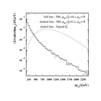
Further reduction of the SM background can be achieved by a cut in the invariant mass distribution of the $\gamma\gamma$ pairs. As illustrated in Fig. 1, the invariant mass distribution for the SM background contribution is a decreasing function of the $\gamma\gamma$ invariant mass while the anomalous contribution first increases with the $\gamma\gamma$ invariant mass reaching its maximum value at $m_{\gamma\gamma}\sim 1000$ GeV and then decreases. Consequently, in order to enhance the WBF signal for the anomalous couplings we imposed the following additional cut in the diphoton invariant mass spectrum

$$400\text{ GeV }\leq m_{\gamma\gamma}\leq 2500\text{ GeV.}$$ (31)

Figure 1: Normalized invariant mass distribution of the $\gamma\gamma$ pair for the reaction $pp\to\gamma\gamma jj$.

We present in Table 1 the values for $\sigma_{\text{ano}}$ for each of the independent linear combination of anomalous couplings in Eqs. (18) and (19) after applying the cuts in Eqs. (29)–(31). These results were obtained using $\sqrt{\hat{s}}$ as the factorization scale in the parton distribution functions. We have further assumed a 85% detection efficiency of isolated photons, leptons and jet-tagging. With this the efficiency for reconstructing the final state $j+j+\gamma+\gamma$ is $(0.85)^{4}\approx$ 52% which is included in the results presented in Tables 1 and 2. The interference terms ($\sigma_{\text{inter}}$) between the anomalous and SM amplitudes turn out to be negligible. As expected the $WW$ fusion process due to ${{\cal W}}_{0}^{\gamma}$ (${{\cal W}}_{c}^{\gamma}$) leads to a larger anomalous contribution (by a factor $\simeq 2.5$) than the $ZZ$ fusion ones due to the ${{\cal Z}}_{0}^{\gamma}$ (${{\cal Z}}_{c}^{\gamma}$).

Coupling Constant	$\sigma_{\text{ano}}$ (pb $\times$ GeV4)
$k^{\gamma}_{0}$	$2.1\times 10^{7}$
$k^{\gamma}_{c}$	$1.5\times 10^{6}$
$k^{\gamma}_{1}$	$6.0\times 10^{6}$
$k^{\gamma}_{23}$	$4.3\times 10^{5}$

Table 1: Results for $\sigma_{\text{ano}}$ for process Eq. (1) [see Eq. (27)]. We considered $n=5$ and $\Lambda_{u}=2.5$ TeV; see Eq. (25). All results include the effect of the cuts in Eq. (29), (III.1), and (31) as well as photon detection and jet-tagging efficiencies.

The evaluation of the SM background ($\sigma_{\text{sm}}$) deserves some special care since it has a large contribution from QCD subprocesses whose size depends on the choice of the renormalization scale used in the evaluation of the QCD coupling constant, $\alpha_{s}(\mu_{R})$, as well as on the factorization scale $\mu_{F}$ used for the parton distribution functions. To estimate the uncertainty associated with these choices, we have computed $\sigma_{\text{sm}}$ for two sets of renormalization scales, which we label as $\mu_{R1,2}(\xi)$, and for several values of $\mu_{F}$. $\mu_{R1}(\xi)$ is defined such that $\alpha_{s}^{2}(\mu_{R1}(\xi))=\alpha_{s}(\xi p_{T}^{j1})\alpha_{s}(\xi pt_{T}^{j2})$ where $p_{T}^{j1}$ and $p_{T}^{j2}$ are the transverse momentum of the tagging jets and $\xi$ is a free parameter varied between 0.1 and 10. The second choice of renormalization scale set is $\mu_{R2}(\xi)=\xi\sqrt{\hat{s}}/2$, with $\sqrt{\hat{s}}$ being the subprocess center–of-mass energy.

	$\sigma_{\text{sm}}$ (fb)
	$\mu_{R}=\mu_{R1}(\xi)$			$\mu_{R}=\mu_{R2}(\xi)$
$\xi$	$\mu_{F}=\sqrt{\hat{s}}$	$\mu_{F}=p^{T}_{\rm min}$	$\mu_{F}=\sqrt{\hat{s}}/10$	$\mu_{F}=\sqrt{\hat{s}}$	$\mu_{F}=p^{T}_{\rm min}$	$\mu_{F}=\sqrt{\hat{s}}/10$
0.10	3.2	5.3	4.1	1.3	2.2	1.7
0.25	2.2	3.6	2.8	1.1	1.9	1.4
1.00	1.4	2.4	1.9	0.91	1.5	1.2
4.00	1.1	1.8	1.4	0.78	1.3	1.0
10.0	0.94	1.6	1.2	0.71	1.2	0.96

Table 2: Results for $\sigma_{\text{sm}}$ for process Eq. (1); see Eq. (27) and text for details. All results include the effect of the cuts in Eq. (29), (III.1) and (31) as well as photon detection and jet-tagging efficiencies.

In Table 2 we list $\sigma_{\text{sm}}$ for the two sets of renormalization scales and for three values of the factorization scale $\mu_{F}=\sqrt{\hat{s}}$, $\sqrt{\hat{s}}/10$, and $p^{T}_{\rm min}$ where $p^{T}_{\rm min}={\rm min}(p_{T}^{j1},p_{T}^{j2})$. As shown in this table, we find that the predicted SM background can change by a factor of $\sim 8$ depending on the choice of the QCD scales. These results indicate that to obtain meaningful information about the presence of anomalous couplings one cannot rely on the theoretical evaluation of the background. Instead one should attempt to extract the value of the SM background from data in a region of phase space where no signal is expected and then extrapolate to the signal region.

In looking for the optimum region of phase space to perform this extrapolation, one must search for kinematic distributions for which (i) the shape of the distribution is as independent as possible of the choice of QCD parameters. Furthermore, since the electroweak and QCD contributions to the SM backgrounds are of the same order info , this requires that (ii) the shape of both electroweak and QCD contributions are similar. Several kinematic distributions verify condition (i), for example, the azimuthal angle separation of the two tagging jets which was proposed in Ref. Eboli:2000ze to reduce the perturbative QCD uncertainties of the SM background estimation for invisible Higgs searches at LHC. However, the totally different shape of the electroweak background in the present case, renders this distribution useless.

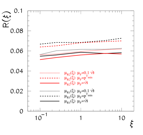
We found that the best sensitivity is obtained by using the $\gamma\gamma$ invariant mass. As can be seen in Fig. 1, the shape of the SM distribution is quite independent of the choice of the QCD parameters. As a consequence most of the QCD uncertainties cancel out in the ratio

$$R(\xi)=\frac{\sigma({400\text{ GeV }<m_{\gamma\gamma}<2500\text{ GeV }})}{\sigma({100\text{ GeV }<m_{\gamma\gamma}<400\text{ GeV }})}\;\;.$$ (32)

This fact is illustrated in Fig. 2 where we plot the value of the ratio $R(\xi)$ for different values of the renormalization and factorization scales. The ratio $R$ is almost invariant under changes of the renormalization scale, showing a maximum variation of the order of $\pm 6$% for a fixed value of the factorization scale. On the other hand, the uncertainty on the factorization scale leads to a maximum variation of 12% in the background estimation. We have also verified that different choices for the structure functions do not affect these results.

Figure 2: Ratio $R(\xi)$ defined in Eq. (32) for the process $pp\to\gamma\gamma jj$ at LHC.

Thus the strategy here proposed is simple: the experiments should measure the number of events in the $\gamma\gamma$ invariant mass window $100<m_{\gamma\gamma}<400$ GeV and extrapolate the results for higher invariant masses using perturbative QCD. According to the results described above we can conservatively assign a maximum “QCD” uncertainty (${\rm QCD}_{\rm unc}$) of $\pm$ 15% to this extrapolation.

In order to estimate the attainable sensitivity to the anomalous couplings we assume that the observed number of events is compatible with the expectations for $\mu_{R1}(\xi=1)$ and $\mu_{F}=\sqrt{\hat{s}}$, so the observed number of events in the signal region coincides with the estimated number of background events obtained from the extrapolation of the observed number of events in the region where no signal is expected; for this choice the number of expected background events is $N_{\rm back}=\sigma_{\text{sm}}{\cal L}$ where ${\cal L}$ stands for the integrated luminosity. For an integrated luminosity of 100 fb^-1 for LHC, this corresponds to $N_{\rm back}=143$. Moreover, we have added in quadrature the statistical error and the QCD uncertainty associated with the backgrounds. Therefore, the 95% limits on the quartic couplings can be obtained from the condition

$$N_{\rm ano}\,=\,\frac{k^{2}_{j}}{\Lambda^{4}}\,\times{\cal L}\,\times\,\sigma_{\rm ano}\leq 1.95\sqrt{N_{\rm back}+(N_{\rm back}\times{\rm QCD}_{\rm unc})^{2}}\;.$$ (33)

For the sake of completeness we show the results on the expected sensitivity using purely statistical errors and for two values of ${\rm QCD}_{\rm unc}$: our most conservative estimate [15 %], and a possible reduced uncertainty (7.5 %), which could be attainable provided NLO QCD calculations are available. Assuming that only one operator is different from zero, so no cancellations are possible, we find

$$|k_{0}^{w,b,m}/\Lambda^{2}|<3.3\,(3.9)\,[4.8]\times 10^{-6}\text{ GeV}^{-2}\;,$$

$$|k_{c}^{w,b,m}/\Lambda^{2}|<1.3\,(1.5)\,[1.8]\times 10^{-5}\text{ GeV}^{-2}\;,$$

$$|k_{1}^{w,b,m}/\Lambda^{2}|<6.2\,(7.2)\,[8.9]\times 10^{-6}\text{ GeV}^{-2}\;,$$ (34)

$$|k_{2}^{w,b,m}/\Lambda^{2}|<2.3\,(2.7)\,[3.3]\times 10^{-5}\text{ GeV}^{-2}\;,$$

$$|k_{3}^{w,m}/\Lambda^{2}|<2.3\,(2.7)\,[3.3]\times 10^{-5}\text{ GeV}^{-2}\;.$$

We notice that the constraint on $k_{2}^{w,b,m}$ and $k_{3}^{w,m}$ are exactly the same as they both modify in the same form and amount the process (1) as seen in Eq. (II).

Finally, let us comment that the limits on $k_{0}^{w,b,m}/\Lambda^{2}$ and $k_{c}^{w,b,m}/\Lambda^{2}$ can be directly translated on constraints on the coefficients $a_{0,c}$, of the operators introduced in Ref. bel:bou with the substitution $a_{0,c}=4g^{2}k_{0,c}^{\gamma}$ (see Eq. (18)).

III.2 $p+p\to j+j+\gamma+l^{+}+l^{-}$

This process receives contribution from the four-gauge coupling vertices $ZZZ\gamma$ and $WWZ\gamma$ as well as from $ZZ\gamma\gamma$ and $WW\gamma\gamma$. We have imposed a minimal set of cuts to guarantee that the photons, charged leptons and jets are detected and isolated from each other:

$$p_{T}^{j_{1(2)}}\geq 40(20)\text{ GeV }\;\;\;\;\hbox{,}\;\;\;\;p_{T}^{\ell}\geq 25\text{ GeV }\;\;\;\;\hbox{,}\;\;\;\;E_{T}^{\gamma}\geq 25\text{ GeV }\;,$$

$$|\eta_{\gamma,\ell}|\leq 2.5\;\;\;\;\hbox{,}\;\;\;\;|\eta_{j_{(1,2)}}|<5.0\;,$$

$$|\eta_{j_{1}}-\eta_{j_{2}}|>4.4\;\;\;\;\hbox{,}\;\;\;\;\eta_{j_{1}}.\eta_{j_{2}}<0\;,$$ (35)

$$\text{min}\{\eta_{j_{1}},\eta_{j_{2}}\}+0.7<\eta_{\gamma,\ell}<\text{max}\{\eta_{j_{1}},\eta_{j_{2}}\}-0.7\;,$$

$$\Delta R_{jj~{}(j\gamma,j\ell)}>0.7\;\;\;\;\hbox{,}\;\;\;\;\Delta R_{\ell^{+}\ell^{-}(\gamma\ell)}>0.4\;.$$

Furthermore, in order to single out the events containing $Z^{0}$ bosons and to enhance the WBF signal for the anomalous couplings $ZZZ\gamma$ and $WWZ\gamma$ we have imposed the following additional cuts on the lepton-lepton ($m_{\ell\ell}$) and lepton-lepton-photon ($m_{\gamma\ell\ell}$) invariant masses:

$$|m_{\ell\ell}-M_{Z}|\leq 20\text{ GeV }\;\;\;\;\hbox{and}\;\;\;\;400\text{ GeV }\leq m_{\gamma\ell\ell}\leq 2500\text{ GeV.}$$ (36)

In Table 3 we display the values of $\sigma_{\text{ano}}$ after cuts for each anomalous couplings $k_{i}^{j}$ in Eq. (II), with $\mu_{F}=\sqrt{\hat{s}}$. These results include the effect of detection and tagging efficiencies; 85% efficiency for detecting isolated photons and leptons and for tagging a jets. With this, the efficiency for reconstructing the final state $j+j+\gamma+l^{+}\,l^{-}$ is $(0.85)^{5}\approx$ 44%. We have added the contributions from final states containing electrons and muons. Once again, we verified that the interference terms $\sigma_{\text{inter}}$ are negligible.

A detailed study of the results in terms of the different Lorentz structures involved show that the invariant mass cut on the lepton-lepton invariant mass suppresses the contributions from the $W^{+}W^{-}\gamma\gamma$ Lorentz structures ${\cal W}_{0}^{\gamma}$ and ${\cal W}_{c}^{\gamma}$ in relation to those containing the $VVZ\gamma$ and $ZZ\gamma\gamma$ quartic vertices ($V=W$ or $Z$). However, we find that none of the Lorentz structures involving these vertices is clearly dominant and that there are important interference effects between the different Lorentz structures contributing to the same anomalous operator, which are the order of 10–30% and can be destructive or constructive.

Coupling Constant	$\sigma_{\text{ano}}$ (pb $\times$ GeV4)
$k_{0}^{w}$	$4.6\times 10^{7}$
$k_{c}^{w}$	$9.2\times 10^{6}$
$k_{1}^{w}$	$2.9\times 10^{7}$
$k_{2}^{w}$	$1.3\times 10^{7}$
$k_{3}^{w}$	$1.0\times 10^{7}$
$k_{0}^{b}$	$6.9\times 10^{6}$
$k_{c}^{b}$	$1.9\times 10^{6}$
$k_{1}^{b}$	$4.7\times 10^{6}$
$k_{2}^{b}$	$1.8\times 10^{6}$
$k_{0}^{m}$	$1.1\times 10^{7}$
$k_{c}^{m}$	$3.2\times 10^{6}$
$k_{1}^{m}$	$9.0\times 10^{6}$
$k_{2}^{m}$	$4.3\times 10^{6}$
$k_{3}^{m}$	$3.6\times 10^{6}$

Table 3: Results for $\sigma_{\text{ano}}$ for the process (2); see Eq. (27). $\sigma_{\text{ano}}$ is obtained for the anomalous coupling $k_{i}^{j}/\Lambda^{2}$ in units of GeV^-2. We considered $n=5$ and $\Lambda_{u}=2.5$ TeV; see Eq. (26).

The evaluation of the SM background in this case is also subject to QCD uncertainties, as in the previous reaction. We found that for our reference value $\mu_{R1}(\xi=1)$ and $\mu_{F}=\sqrt{\hat{s}}$

$$\sigma_{\rm sm}=0.10\;{\rm fb.}$$ (37)

Changes in the factorization and renormalization scales, can modify this prediction by a factor $\sim$ 5. Thus, again, the best strategy to accurately determine the sensitivity to the anomalous coupling is to extract the value of the SM background from data in a region of phase space where no signal is expected and then extrapolate to the signal region. Following the discussion in the previous section, we find that the $\ell^{+}\ell^{-}\gamma$ invariant mass distribution is suitable to estimate the SM background and reduce the QCD uncertainties. We have defined the ratio

$$R(\xi)=\frac{\sigma({400\text{ GeV }<m_{\ell\ell\gamma}<2500\text{ GeV }})}{\sigma({100\text{ GeV }<m_{\ell\ell\gamma}<400\text{ GeV }})}\;\;,$$ (38)

and evaluated the behavior of $R(\xi)$ under changes of the renormalization and factorization scales. We determined that $R(\xi)$ can be known within an accuracy of $\pm$ 15% when we use leading order calculations.

In order to extract the attainable limits on the anomalous couplings we assumed a luminosity of ${\cal L}=100$ fb^-1 and that the observed number of events is compatible with the expectations for $\mu_{R1}(\xi=1)$ and $\mu_{F}=\sqrt{\hat{s}}$, i.e. the expected number of background events in the signal region is $N_{\rm back}=10$. We have added to the statistical error associated with this background the theoretical error associated to the uncertainty in the extrapolation of the background. However, given the limited statistics, the sensitivity is dominated by the statistical error. The 95% C.L. constraints on the anomalous couplings are

$$|k_{0}^{w}/\Lambda^{2}|<1.2\times 10^{-6}\text{ GeV}^{-2}\;\;,$$

$$|k_{c}^{w}/\Lambda^{2}|<2.8\times 10^{-6}\text{ GeV}^{-2}\;\;,$$

$$|k_{1}^{w}/\Lambda^{2}|<1.5\times 10^{-6}\text{ GeV}^{-2}\;\;,$$

$$|k_{2}^{w}/\Lambda^{2}|<2.3\times 10^{-6}\text{ GeV}^{-2}\;\;,$$

$$|k_{3}^{w}/\Lambda^{2}|<2.6\times 10^{-6}\text{ GeV}^{-2}\;\;,$$

$$|k_{0}^{b}/\Lambda^{2}|<3.2\times 10^{-6}\text{ GeV}^{-2}\;\;,$$ (39)

$$|k_{c}^{b}/\Lambda^{2}|<6.0\times 10^{-6}\text{ GeV}^{-2}\;\;,$$

$$|k_{1}^{b}/\Lambda^{2}|<3.8\times 10^{-6}\text{ GeV}^{-2}\;\;,$$

$$|k_{2}^{b}/\Lambda^{2}|<6.3\times 10^{-6}\text{ GeV}^{-2}\;\;,$$

$$|k_{0}^{m}/\Lambda^{2}|<2.6\times 10^{-6}\text{ GeV}^{-2}\;\;,$$

$$|k_{c}^{m}/\Lambda^{2}|<4.7\times 10^{-6}\text{ GeV}^{-2}\;\;,$$

$$|k_{1}^{m}/\Lambda^{2}|<2.8\times 10^{-6}\text{ GeV}^{-2}\;\;,$$

$$|k_{2}^{m}/\Lambda^{2}|<4.0\times 10^{-6}\text{ GeV}^{-2}\;\;,$$

$$|k_{3}^{m}/\Lambda^{2}|<4.4\times 10^{-6}\text{ GeV}^{-2}\;\;.$$

which have been obtained including a 15% QCD uncertainty, However, to the precision quoted, the impact of this uncertainty is minimal.

Comparing the limits in Eqs. (39) with the corresponding ones from the process (1) in Eq. (34) we see that, despite the limited statistics, the presence of the $VVZ\gamma$ vertex ($V=W$ or $Z$) makes the process $pp\to jj\gamma l^{+}l^{-}$ most sensitive to the presence of NP leading to anomalous four-vector couplings which respect the $SU(2)_{L}\times U(1)_{Y}$ gauge invariance as well as the $SU(2)_{\rm c}$ custodial symmetry. One of the reasons for the process $pp\to jj\gamma l^{+}l^{-}$ to be more sensitive to anomalous interactions is that almost all Lorentz structures lead similar contributions and that more Lorentz structures contribute to this reaction than in $pp\to jj\gamma\gamma$ for a given effective operator.

One must keep in mind, however, that the results in Eqs. (34) and (39) were obtained under the assumption that only one operator is different from zero, so no cancellations were possible. If cancellations are allowed the process (1) may become the most sensitive one to the presence of the relevant photonic quartic operators.

IV Discussion

We are just beginning to test the SM predictions for the quartic vector boson interactions. Due to the limited available center–of–mass energy, the first couplings to be studied should contain photons. In particular, the direct searches at LEPII have lead to constraints of the order $|\frac{k_{i}^{j}}{\Lambda^{2}}|\lesssim{\cal O}(10^{-2}\;{\rm GeV^{-2})}$ for the couplings in Eq. (II), and no significantly better sensitivity is expected from searches at Tevatron. Anomalous quartic couplings contribute at the one–loop level to the $Z$ physics our:vvv via oblique corrections as they modify the $W$, $Z$, and photon two–point functions. Consequently they can be indirectly constrained by precision electroweak data to $|\frac{k_{i}^{j}}{\Lambda^{2}}|\lesssim{\cal O}(10^{-4}\;{\rm GeV^{-2})}$.

Higher energy colliders will be able to test quartic gauge couplings involving photons as well as to probe non-photonic vertices $VVV^{\prime}V^{\prime}$ ($V,V^{\prime}=W$ or $Z$) vvvv . Even at LHC energies, due to phase space limitations, the best experimental sensitivity is expected for couplings involving photons which can be part of the final state. Moreover, in the event that a departure from the SM predictions is observed, inference of the underlying dynamics can only be obtained by comparing the observations in different channels, for instance between those involving triple and quartic-gauge couplings. In this respect it will also be important to know whether NP reveals itself in the form of anomalous four-gauge couplings involving only weak gauge bosons or in those involving photons or in both. For instance, in the framework of chiral lagrangians, where no light Higgs state is observed, the photonic four vertices are expected to be suppressed with respect to the non-photonic ones since they appear one order higher in the momentum expansion. An anomalous signal only in the photonic couplings could indicate that there are additional symmetries forbidding the non-photonic vertices.

With this motivation, in this work we have analyzed the production of two jets in association with a photon pair, or with a photon and a $\ell^{+}\ell^{-}$ pair at LHC as tests of anomalous bosonic quartic couplings involving one or two photons. In this study we have taken careful account of the theoretical uncertainties associated with the evaluation of the SM background. We have proposed the best strategy to estimate the expected SM background by extrapolation of the data taken in a region of phase space where no signal is expected, minimizing the theoretical uncertainty associated to this extrapolation. The final sensitivity to the different couplings is given in Eqs. (34) and (39). In particular, we found that in the framework of $SU(2)_{L}\times U(1)_{Y}$ gauge invariant NP in which the deviations from the SM prediction for the $VV\gamma\gamma$ vertices are related to the strength of the anomalous $VVZ\gamma$ vertex, the process $pp\to jj\gamma l^{+}l^{-}$ is the most sensitive to all possible operators, despite the limited statistics, barring possible cancellations. It can lead to constraints $|\frac{k_{i}^{j}}{\Lambda^{2}}|\lesssim 1.2$–$6.3\times 10^{-6}\;{\rm GeV^{-2}}$.

In conclusion we have shown that the study of the processes (1) and (2) at LHC can test quartic anomalous couplings that are four orders of magnitude weaker than the existing limits from direct searches and two orders of magnitude weaker than any indirect constraints. It is interesting to notice that if no signal is found the LHC will lead to limits that are similar to the ones that could be attainable at an $e^{+}e^{-}$ collider operating at $\sqrt{s}=500$ GeV with a luminosity of 300 fb^-1 Belanger:1999aw ; nlc .

References

• (1) For a review see: H. Aihara et al., Anomalous gauge boson interactions in Electroweak Symmetry Breaking and New Physics at the TeV Scale, edited by T. Barklow, S. Dawson, H. Haber and J. Seigrist, (World Scientific, Singapore, 1996), p. 488 [hep-ph/9503425].
• (2) K. Gounder, CDF Collaboration, hep-ex/9903038; B. Abbott et al., DØ Collaboration, Phys. Rev.  D62, 052005 (2000).
• (3) P. Achard et al. [L3 Collaboration], Phys. Lett. B 547, 151 (2002); P. Abreu et al. [DELPHI Collaboration], Phys. Lett. B 502, 9 (2001); A. Heister et al. [ALEPH Collaboration], Eur. Phys. J. C 21, 423 (2001).
• (4) LEP Electroweak Working Group and and SLD Heavy Flavor Group hep-ex/0212036.
• (5) P. Achard et al. [L3 Collaboration], Phys. Lett. B 527, 29 (2002); G. Abbiendi et al. [OPAL Collaboration], hep-ex/0309013.
• (6) G. Belanger, F. Boudjema, Y. Kurihara, D. Perret-Gallix and A. Semenov, Eur. Phys. J. C 13, 283 (2000).
• (7) W. J. Stirling and A. Werthenbach, Phys. Lett. B466, 369 (1999);
• (8) O. J. Eboli, M. C. Gonzalez-Garcia, S. M. Lietti and S. F. Novaes, Phys. Rev. D 63, 075008 (2001).
• (9) P. J. Dervan, A. Signer, W. J.  Stirling, and A. Werthenbach , J. Phys. G26, 607 (2000).
• (10) O. J. P. Éboli, M. C. Gonzalez–Garcia, and J. K. Mizukoshi, Phys. Rev. D58, 034008 (1998); T. Han, H.-J. He, and C.-P. Yuan, Phys. Lett. B422, 294 (1998); V. Barger, K. Cheung, T. Han, and R. J. N. Philips, Phys. Rev. D52, 3815 (1995); E. E. Boos, H. J.  He , W.  Kilian, A. Pukhov, and P. M. Zerwas, Phys. Rev. D57, 1553 (1997); J. Bagger, S. Dawson, and G. Valencia, Nucl. Phys. B399, 364 (1993); A. Dobado, D. Espriu, and M. J. Herrero, Z. Phys. C50, 205 (1991); A. S. Belyaev, et al., Phys. Rev. D59, 015022 (1999); A. Dobado and M. T. Urdiales, Z. Phys. C17, 965 (1996); J. R. Pelaez, Phys. Rev. D55, 4193 (1997).
• (11) G. Bélanger and F. Boudjema, Phys. Lett. B288,201 (1992); W. J. Stirling and A. Werthenbach, Eur. Phys. J. C14, 103 (2000).
• (12) G. Bélanger and F. Boudjema, Phys. Lett. B288, 210 (1992).
• (13) O. J. P. Éboli, M. B. Magro, P. G. Mercadante, and S. F. Novaes, Phys. Rev. D52, 15 (1995).
• (14) O. J. P. Éboli, M. C. Gonzalez-Garcia, and S. F. Novaes, Nucl. Phys. B411, 381 (1994).
• (15) T. Appelquist and C. Bernard, Phys. Rev. D22, 200 (1980); A. Longhitano, Phys. Rev. D22, 1166 (1980); Nucl. Phys. B188, 118 (1981).
• (16) T. Stelzer and W. F. Long, Comput. Phys. Commun. 81, 357 (1994).
• (17) H. Murayama, I. Watanabe, and K. Hagiwara, KEK report 91-11 (unpublished).
• (18) The electroweak contribution to the total SM background is approximately 25% for $\mu_{R1}(\xi=1)$ and $\mu_{F}=\sqrt{\hat{s}}$.
• (19) O. J. Eboli and D. Zeppenfeld, Phys. Lett. B 495, 147 (2000).