The MSSM fine tuning problem: a way out

As is well known, electroweak breaking in the MSSM requires substantial fine-tuning, mainly due to the smallness of the tree-level Higgs quartic coupling, $\lambda_{\rm tree}$. Hence the fine tuning is efficiently reduced in supersymmetric models with larger $\lambda_{\rm tree}$, as happens naturally when the breaking of SUSY occurs at a low scale (not far from the TeV). We show, in general and with specific examples, that a dramatic improvement of the fine tuning (so that there is virtually no fine-tuning) is indeed a very common feature of these scenarios for wide ranges of $\tan\beta$ and the Higgs mass (which can be as large as several hundred GeV if desired, but this is not necessary). The supersymmetric flavour problems are also drastically improved due to the absence of RG cross-talk between soft mass parameters.

October 2003

IFT-UAM/CSIC-03-40

IEM-FT-233/03

hep-ph/0310137

1 The supersymmetric fine tuning problem

One of the most attractive features of supersymmetry (SUSY) [1] is that it provides a radiative mechanism for the electroweak (EW) breaking [2]. Large radiative corrections associated to the top Yukawa coupling destabilize the origin of the Higgs potential and induce quite naturally a non trivial minimum at the right scale, ${v}=246$ GeV, if the mass terms that encode the soft breaking of SUSY are not far from the EW scale. This crucial success of SUSY has been undermined in recent times by a worrisome fine tuning problem [3]-[14]: the non observation of the Higgs boson and of superpartners sets significant lower bounds on the size of the soft breaking terms in such a way that a delicate cancellation is generically required to avoid too large a value for $v$.

Let us briefly recall how this comes about in the ordinary Minimal Supersymmetric Standard Model (MSSM). In the MSSM the Higgs sector consists of two $SU(2)_{L}$ doublets, $H_{1}$, $H_{2}$. The (tree-level) scalar potential for the neutral components, $H^{0}_{1,2}$, of these doublets reads

$$V^{\rm MSSM}(H^{0}_{1},H^{0}_{2})=m_{1}^{2}|H_{1}^{0}|^{2}+m_{2}^{2}|H_{2}^{0}|^{2}-2m_{3}^{2}H_{1}^{0}H^{0}_{2}+\frac{1}{8}(g^{2}+g_{Y}^{2})(|H^{0}_{1}|^{2}-|H^{0}_{2}|^{2})^{2},$$ (1)

with $m_{1,2}^{2}=\mu^{2}+m_{H_{1,2}}^{2}$ and $m_{3}^{2}=B\mu$, where $m_{H_{i}}^{2}$ and $B$ are soft masses and $\mu$ is the Higgs mass term in the superpotential, $W\supset\mu H_{1}\cdot H_{2}$. Minimization of $V^{\rm MSSM}$ leads to a vacuum expectation value (VEV) $v^{2}\equiv 2(\langle H^{0}_{1}\rangle^{2}+\langle H^{0}_{2}\rangle^{2})$ and thus to a mass for the $Z^{0}$ gauge boson, $M_{Z}^{2}=\frac{1}{4}(g^{2}+g_{Y}^{2})v^{2}$, given by

$$\frac{M_{Z}^{2}}{2}=-\mu^{2}+\frac{m_{H_{1}}^{2}-m_{H_{2}}^{2}\tan^{2}\beta}{\tan^{2}\beta-1}\ ,$$ (2)

where $\tan\beta\equiv\langle H^{0}_{2}\rangle/\langle H^{0}_{1}\rangle$. The quantities in the r.h.s. of (2) are to be understood as evaluated at low energy. They are related to more fundamental parameters at a higher scale, $\Lambda_{UV}$ (typically $\Lambda_{UV}\equiv$ $M_{GUT}$ or $M_{P}$, but there are other possibilities) by renormalization group equations (RGEs). The MSSM RGEs for the mass parameters in (2) are coupled to those of other soft terms, e.g. gaugino masses, stop masses, trilinear terms, etc., so $M_{Z}^{2}$ can be expressed as a linear combination of initial (UV) mass–squared parameters with coefficients that can be calculated by integrating the RGEs. For example, for large $\tan\beta$ (the best situation for the fine tuning problem, as will be clear in the discussion) and $\Lambda_{UV}=M_{GUT}=1.4\times 10^{16}$ GeV we get [15]:

$$M_{Z}^{2}\simeq-2.02\mu^{2}+3.57M^{2}+0.07m^{2}+0.22A^{2}+0.75AM\ ,$$ (3)

where $M,m,A$ are the gaugino mass, scalar soft mass and trilinear soft term respectively, taken universal for simplicity. From the previous equation it is apparent that, even for moderate values of the initial parameters (i.e. significantly smaller than 1 TeV), some of the terms in the r.h.s. are much larger than $M_{Z}^{2}$, thus a non-trivial cancellation among them (and therefore a fine tuning) is necessary in general.

The previous fine tuning can be avoided in two ways. The first is that the required cancellation among different terms is “miraculously” provided by the fundamental theory underlying the MSSM, e.g. string theory. This certainly would be a fortunate accident since the cancellation not only involves the sizes of the various soft breaking terms (and the $\mu$-parameter), which arise from the unknown SUSY breaking (SUSY) mechanism, but also the different magnitudes of the coefficients in (3), which have to do with the RG running between the initial and the low energy scale. These quantities have such a different physical origin that it is difficult to imagine a fundamental reason why they should be correlated in the correct way to enforce a cancellation. As a matter of fact, the analyses in the literature [11, 13, 16] of many superstring, superstring-inspired and supergravity models do not find such correlations.

The second way to avoid the fine tuning would be that each term in the r.h.s. of (3) is not larger than a few times $M_{Z}^{2}$. But, if the soft masses are lowered at will, the masses of SUSY particles will fall below their experimental bounds. The problem is especially acute for the LEP bound on the Higgs mass, $m_{h}\geq 115$ GeV [17] as has been stressed by a number of authors [9, 10, 11, 12]. This can be easily understood by writing the tree-level and the dominant 1-loop correction [18] to the theoretical upper bound on $m_{h}$ in the MSSM:

$$m_{h}^{2}\leq M_{Z}^{2}\cos^{2}2\beta+{3m_{t}^{4}\over 2\pi^{2}v^{2}}\log{M_{\rm SUSY}^{2}\over m_{t}^{2}}+...$$ (4)

where $m_{t}$ is the (running) top mass ($\simeq 167$ GeV for $M_{t}=174$ GeV) and $M_{\rm SUSY}$ is an average of stop masses. Since the experimental lower bound on $m_{h}$ exceeds the tree-level contribution, the radiative corrections must be responsible for the difference, and this translates into a lower bound on $M_{\rm SUSY}$:

$$M_{\rm SUSY}\;\stackrel{{\scriptstyle>}}{{{}_{\sim}}}\;e^{-2.1\cos^{2}2\beta}e^{\left({m_{h}}/{62\ {\rm GeV}}\right)^{2}}m_{t}\;\stackrel{{\scriptstyle>}}{{{}_{\sim}}}\;3.8\ m_{t}\ ,$$ (5)

where the last figure corresponds to $m_{h}=115$ GeV and large $\tan\beta$. Hence $M_{\rm SUSY}^{2}$ must be already more than 40 times bigger than $M_{Z}^{2}$ and this number increases exponentially for larger (smaller) $m_{h}$ ($\tan\beta$). On the other hand $M_{\rm SUSY}$ is itself a low energy quantity that has a dependence on the initial soft masses analogous to eq. (3):

$$M_{\rm SUSY}^{2}\simeq 3.36M^{2}+0.49m^{2}-0.05A^{2}-0.19AM+m_{t}^{2}+({\rm D-terms})\ .$$ (6)

Roughly, $M_{\rm SUSY}^{2}$ has a magnitude similar to the main positive contribution in the r.h.s. of (3), which then implies that some of the terms in that sum are at least $\sim$ 45 times larger than $M_{Z}^{2}$, showing up the fine tuning. (The evaluation of the MSSM fine tuning is refined in the next section.)

Several ways to alleviate the SUSY fine tuning problem have been explored in the literature, e.g. invoking a correlation between parameters based on some theoretical construction as mentioned above [11, 13, 16]. The improvement, however, is never dramatic. Here we take a different path: the fine tuning can be alleviated or, indeed, eliminated if the supersymmetric theory has larger tree-level quartic Higgs couplings than the conventional one [see eq. (1)]. In this way, the size of the various contributions to $M_{Z}^{2}$ [eq. (3) for the MSSM] is dramatically lowered and, besides, the soft breaking terms do not need to be large since the radiative corrections are no longer necessary to explain the Higgs mass. We show here (building on a previous observation in [19]) how this happens naturally if the SUSY breaking occurs at a low scale (not far from the TeV).

The paper is organized as follows: In sect. 2 we discuss and identify the causes for the abnormally large fine tuning of the MSSM, envisaging possible cures. In sect. 3 we consider low scale SUSYscenarios, evaluating the corresponding fine tuning and showing that it can be drastically smaller than in the MSSM. In sect. 4 we offer a concrete and realistic realization of the mechanism in a specific model. In sect. 5 we make some concluding remarks. Finally, in appendix A we present formulas for measuring the fine tuning in generic scenarios, while appendix B discusses the limits that Higgs searches at LEP impose on the parameters of the kind of models we consider.

2 Underlying causes and possible cures

It is interesting to note that the fine tuning in the MSSM is much more severe than what simple dimensional arguments suggest. To show this we quantify the fine tuning following Barbieri and Giudice [3]: we write the Higgs VEV as a function of the initial parameters $p_{\alpha}$ of the model under study, $v^{2}=v^{2}(p_{1},p_{2},\cdots)$, and define $\Delta_{p_{\alpha}}$, the fine tuning parameter associated to $p_{\alpha}$, by

$${\delta M_{Z}^{2}\over M_{Z}^{2}}={\delta v^{2}\over v^{2}}=\Delta_{p_{\alpha}}{\delta p_{\alpha}\over p_{\alpha}}\ ,$$ (7)

where $\delta M_{Z}^{2}$ ($\delta v^{2}$) is the change induced in $M_{Z}^{2}$ ($v^{2}$) by a change $\delta p_{\alpha}$ in $p_{\alpha}$. Roughly speaking $\Delta^{-1}_{p_{\alpha}}$ measures the probability of a cancellation among terms of a given size to obtain a result which is $\Delta_{p_{\alpha}}$ times smaller. Absence of fine tuning requires that $\Delta_{p_{\alpha}}$ should not be larger that ${\cal O}(10)$.

The parameter that usually requires the largest fine tuning is $\mu^{2}$ because, due to the negative sign of its contribution in eqs. (2, 3), it has to compensate the (globally positive and large) remaining contributions. Therefore we will focus on $\Delta_{\mu^{2}}$. For large $\tan\beta$ and $m_{h}=115$ GeV the required universal soft mass is $m=M=A\simeq 325$ GeV, according to eqs. (4, 6). When these figures are plugged in eq. (3) and the fine tuning is evaluated according to eq. (7) one obtains $\Delta_{\mu^{2}}\sim 55$. Note that this corresponds to using the tree-level potential (1), evaluated at a low scale. If one refines (1) by including the dominant logarithmic corrections at 1-loop from the top-stop sector (see appendix A) this figure gets down [4, 5] to $\sim 35$.

Now, one could naively expect that if the soft parameters had a size $m_{\rm soft}^{2}\sim av^{2}$, the fine tuning would be $\Delta\sim a$, but for the MSSM one gets $\Delta\stackrel{{\scriptstyle>}}{{{}_{\sim}}}20a$, as can be checked from the previous numbers. In this sense the fine tuning of the MSSM is abnormally large. To understand the reasons for this, let us write the generic Higgs potential along the breaking direction as

$$V={1\over 2}m^{2}v^{2}+{1\over 4}\lambda v^{4}\ ,$$ (8)

where $\lambda$ and $m^{2}$ are functions of the $p_{\alpha}$ parameters and $\tan\beta$, in particular

$$m^{2}=c_{\beta}^{2}\,m_{1}^{2}(p_{\alpha})+s_{\beta}^{2}\,m_{2}^{2}(p_{\alpha})-s_{2\beta}\,m_{3}^{2}(p_{\alpha})\ .$$ (9)

Minimization of (8) leads to

$$v^{2}={-m^{2}\over\lambda}\ .$$ (10)

Clearly, the larger the size of the individual $m_{i}^{2}$ and the smaller $\lambda$, the more severe the fine tuning: $\Delta\sim{\tt m_{i}^{2}}/(\lambda v^{2})$, where ${\tt m_{i}^{2}}$ are the (potentially large) individual contributions to $m_{i}^{2}$. For the MSSM, $\lambda$ turns out to be quite small:

$$\lambda_{\rm MSSM}={1\over 8}(g^{2}+g_{Y}^{2})\cos^{2}2\beta\ \simeq\ {1\over 15}\cos^{2}2\beta\ ,$$ (11)

which already implies a fine tuning $\sim 15$ times larger (for the most favorable case of large $\tan\beta$) than the above naive expectations. The previous $\lambda_{\rm MSSM}$ was evaluated at tree-level but radiative corrections make $\lambda$ larger, thus reducing the fine tuning. The ratio $\lambda_{\rm tree}/\lambda_{\rm 1-loop}$ is basically the ratio $(m_{h}^{2})_{\rm tree}/(m_{h}^{2})_{\rm 1-loop}$, so for large $\tan\beta$ and $m_{h}=115$ GeV the previous factor 15 is reduced by a factor $M_{Z}^{2}/m_{h}^{2}$ down to $\sim 9$. Finally, for the MSSM (with large $\tan\beta$ and $\Lambda_{UV}=M_{GUT}$)

$$m^{2}=m_{1}^{2}c^{2}_{\beta}+m_{2}^{2}s^{2}_{\beta}-m_{3}^{2}s_{2\beta}\simeq 1.01\mu^{2}-2.31\tilde{m}^{2}\ ,$$ (12)

where we have set $A=M=m=\tilde{m}$ for simplicity. The presence of a sizeable RG coefficient in front of $\tilde{m}^{2}$ implies that, for a given magnitude of the latter, the required cancellation must be (in this case) $\sim 2.31$ times more accurate than naive expectations so, finally the factor 9 is enhanced to $\sim 20$. Notice that those large RG coefficients are a consequence of the radiative mechanism of EW breaking, hence if the EW breaking were at tree level the fine tuning would be reduced.

From the above discussion it is important to notice that, although for a given size of the soft terms the radiative corrections reduce the fine tuning, the requirement of sizeable radiative corrections implies itself large soft terms, which in turn worsens the fine tuning. More precisely, for the MSSM $\delta_{\rm rad}\lambda\propto\log(M_{\rm SUSY}/m_{t})$, so $\lambda$ can only be radiatively enhanced by increasing $M_{\rm SUSY}$, and thus the individual ${m}_{i}^{2}$. A given increase in $M_{\rm SUSY}$ reflects linearly in ${m}_{i}^{2}$ and only logarithmically in $\lambda$, so the fine tuning $\Delta\sim{\tt m_{i}^{2}}/(\lambda v^{2})$ gets usually worse. As discussed in sect. 1, for the MSSM $(m_{h})_{\rm tree}<(m_{h})_{\rm exp}$, hence sizeable radiative corrections are in fact mandatory and the fine tuning is consequently aggravated. As a consequence, the fine tuning increases exponentially for increasing (decreasing) $m_{h}$ ($\cos^{2}2\beta$) as indicated by eq. (5).

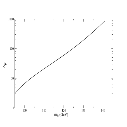
Figure 1: Fine tuning in the MSSM (measured by $\Delta_{\mu^{2}}$) as a function of the Higgs mass (in GeV) for $\tan\beta=10$.

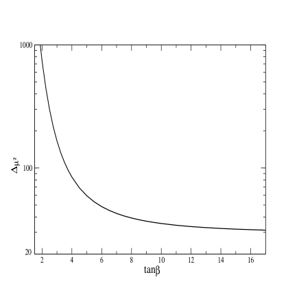
Figure 2: Lower bound on the MSSM fine tuning ($\Delta_{\mu^{2}}$) as a function of $\tan\beta$ from the LEP bound $m_{h}\geq 115$ GeV.

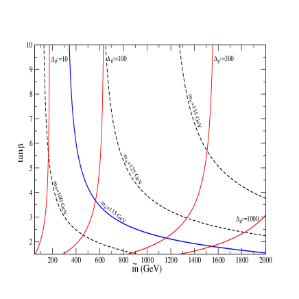
Figure 3: Fine tuning in the MSSM (measured by $\Delta_{\mu^{2}}$, solid lines) in the $(\tilde{m},\tan\beta)$ plane. Dashed lines are contour lines of constant Higgs mass.

Let us illustrate the previous discussion in a more quantitative way. In fig. 1 we plot $\Delta_{\mu^{2}}$, evaluated at one-loop, as a function of the Higgs boson mass, $m_{h}$, for $\tan\beta=10$ (such large value of $\tan\beta$ minimizes the fine tuning, as discussed above). We only include the dominant one-loop correction to $m_{h}$, as shown in eq. (4), and make the simplifying assumption that the soft parameters are universal at the GUT scale. Although the fine tuning can be made smaller in non-universal cases, figure 1 shows the typical size of $\Delta_{\mu^{2}}$ in the MSSM. As expected from the previous discussions, $\Delta_{\mu^{2}}$ grows exponentially for increasing $m_{h}$. The dependence of $\Delta_{\mu^{2}}$ with $\tan\beta$ is shown in fig. 2 for $m_{h}$ at the LEP bound, $m_{h}=115$ GeV (the optimal choice for the fine tuning). The curve for $\Delta_{\mu^{2}}$ increases exponentially for decreasing $\cos^{2}2\beta$, again as expected. This curve can be interpreted as a LEP lower bound on the MSSM fine tuning.

Finally, fig. 3 shows contour lines of constant $\Delta_{\mu^{2}}$ in the $(\tilde{m},\tan\beta)$ plane, where $\tilde{m}$ is the universal soft mass at $\Lambda_{UV}$. We also plot dashed contour lines of constant $m_{h}$ and the LEP lower bound on $m_{h}$. Again, it is clear how the fine tuning is greater for smaller $\tan\beta$ and how it grows, together with $m_{h}$, for larger $\tilde{m}$. The upper horizontal line and the $m_{h}=115$ GeV contour line correspond to figs. 1 and 2 respectively. It is instructive to examine the behaviour of the lines of constant $\Delta_{\mu^{2}}$ along which $\tilde{m}$ and $m_{h}$ grow asymptotically towards fixed upper limits. For instance, if we insist in having small fine tuning, $\Delta_{\mu^{2}}\stackrel{{\scriptstyle<}}{{{}_{\sim}}}10$, following the $\Delta_{\mu^{2}}=10$ line we conclude that one cannot obtain $\tilde{m}$ larger than $\sim 175$ GeV (which translates into upper bounds on superpartner masses) nor Higgs masses larger than $\simeq 103$ GeV, already ruled out by LEP.

A word of caution should be added about the previous numbers. In general, attempting a very accurate determination of the fine tuning does not make much sense. What precise value of the fine tuning should be considered too high? On top of this, the present experimental uncertainty on the top quark mass, $M_{t}=174.3\pm 5.1$ GeV [21], translates into a significant uncertainty on the fine tuning parameters. For these reasons, in our numerical one-loop estimates of $\Delta_{\mu^{2}}$ we have just included the logarithmic correction to $m_{h}^{2}$ given in eq. (4). This simplification is even more justified in this paper, whose main purpose is to compare the performance of unconventional scenarios with that of the MSSM.

In summary, the fine tuning of the MSSM is at least 20 times more severe than naively expected due, basically, to the smallness of the tree-level Higgs quartic coupling, $\lambda_{\rm tree}$. The problem is worsened by the fact that sizeable radiative corrections (and thus sizeable soft terms) are needed to satisfy the experimental bound on $m_{h}$. This is also due the smallness of $\lambda_{\rm tree}$: if it were bigger, radiative corrections would not be necessary. In consequence, the most efficient way of reducing the fine tuning is to consider supersymmetric models where $\lambda_{\rm tree}$ is larger than in the MSSM. More explicitly, the improvement can be evaluated in the following way. The value of $\Delta_{p}$ for a generic parameter $p$ of a given model has the form [see Appendix A]

$$\Delta_{p}=\frac{p}{m^{2}}\left[\frac{\partial m^{2}}{\partial p}+\frac{v^{2}}{2}\frac{\partial\lambda}{\partial\beta}\frac{d\beta}{dp}+v^{2}\frac{\partial\lambda}{\partial p}\right]\ .$$ (13)

Focusing on the $\mu^{2}$ parameter, and taking into account that the last two terms of (13) are usually suppressed by a factor ${\cal O}(v^{2}/\mu^{2})$, we can write

$$\Delta_{\mu^{2}}\simeq\frac{\mu^{2}}{m^{2}}\frac{\partial m^{2}}{\partial\mu^{2}}\simeq-\frac{\mu^{2}}{\lambda v^{2}}\simeq-2\frac{\mu^{2}}{m_{h}^{2}}\ ,$$ (14)

where we have used the fact that the dependence of the low-energy $m^{2}$ on the initial (UV) $\mu$ parameter is usually dominated by the tree-level contribution. Strictly speaking, $m_{h}^{2}$ in (14) is the Higgs mass matrix element along the breaking direction, but in many cases of interest it is very close to one of the mass eigenvalues. Therefore

$$\Delta_{\mu^{2}}\simeq\Delta_{\mu^{2}}^{\rm MSSM}\left[\frac{m_{h}^{\rm MSSM}}{m_{h}}\right]^{2}\left[\frac{\mu}{\mu^{\rm MSSM}}\right]^{2}\ .$$ (15)

This equation shows the two main ways in which a theory can improve the MSSM fine tuning: increasing $m_{h}$ and/or decreasing $\mu$. The first way corresponds to increasing $\lambda$. The second, for a given $m_{h}$, corresponds to reducing the size of the soft terms (EW breaking requires the size of $\mu^{2}$ to be proportional to the overall size of the soft squared-masses), which is only allowed if radiative contributions are not essential to raise $m_{h}$. Both improvements indeed concur for larger $\lambda_{\rm tree}$.

The possibility of having tree-level quartic Higgs couplings larger than in the MSSM is natural in scenarios in which the breaking of SUSY occurs at a low-scale (not far from the TeV scale) [22, 23, 24, 19]. Besides, in that framework EW breaking takes place essentially at tree-level, which, as noticed above, is also welcome for the fine tuning issue. These ideas are developed in detail in the next sections.

3 Low-scale SUSY breaking

In any realistic breaking of SUSY, there are two scales involved: the SUSYscale, say $\sqrt{F}$, which corresponds to the VEVs of the relevant auxiliary fields in the SUSYsector; and the messenger scale, $M$, associated to the interactions that transmit the breaking (through effective operators suppressed by powers of $M$) to the observable sector. These operators give rise to soft terms (such as scalar soft masses), but also hard terms (such as quartic scalar couplings):

$$m_{\rm soft}^{2}\sim{F^{2}\over M^{2}}\ ,\;\;\;\;\lambda_{\makebox[24.18501pt][l]{$\line(4,1){19.0}$ {\tiny{SUSY}}}}\sim{F^{2}\over M^{4}}\sim{m_{\rm soft}^{2}\over M^{2}}\ .$$ (16)

Phenomenology requires $m_{\rm soft}={\cal O}(1\,{\rm TeV})$, but this does not fix the scales $\sqrt{F}$ and $M$ separately. The MSSM assumption is that there is a hierarchy of scales: $m_{\rm soft}\ll\sqrt{F}\ll M$, so that the hard terms are negligible and the soft ones are the only observable trace of SUSY. However, there is no real need for such a strong hierarchy, so the scales $\sqrt{F}$ and $M$ could well be of similar order (thus not far from the TeV scale). This happens in the so-called low-scale SUSYscenarios. In this framework, the hard terms of eq. (16), are not negligible anymore and hence the SUSYcontributions to the Higgs quartic couplings can be easily larger than the ordinary MSSM value (11). As discussed in the previous section, this is exactly the optimal situation to ameliorate the fine tuning problem.

The messenger scale $M$ may be not far from the EW scale for various reasons. E.g. there could be some massive fields responsible for the SUSYmediation (like in gauge mediation) with masses $\sim M$; or there could be a more fundamental reason, as in models with large extra-dimensions or in supersymmetric Randall-Sundrum models. Instead of sticking to one of these particular examples, it is convenient to describe the observable physics using an effective field-theory approach [23, 19]. Denoting by $T$ the superfield responsible for SUSY, $\langle F_{T}\rangle\neq 0$, and assuming that, apart from the $T$ field, the spectrum is minimal (i.e. the same as in the MSSM), the effective theory is like the SUSY part of the MSSM, plus some effective interactions which include couplings between $T$ and the observable fields, suppressed by powers of $M$. These effective interactions can appear in the superpotential, $W$, as well as in the Kähler potential, $K$, or the gauge kinetic function.

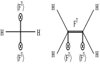
Figure 4: Higgs soft masses and hard quartic couplings that arise from the Kähler operator (17).

As a simple example, suppose that the Kähler potential contains the operator

$$K\ \supset\ -\frac{1}{M^{2}}|T|^{2}|H|^{2}+\cdots$$ (17)

where $H$ denotes any Higgs superfield. Once $F_{T}$ takes a VEV the above nonrenormalizable interaction produces soft terms as well as hard terms, as schematically represented in the diagrams of Fig. 4. Notice that $m_{\rm soft}^{2}\sim|F_{T}|^{2}/M^{2}$, $\lambda_{\makebox[24.18501pt][l]{$\line(4,1){19.0}$ {\tiny{SUSY}}}}\sim|F_{T}|^{2}/M^{4}\sim m_{\rm soft}^{2}/M^{2}$, in agreement with (16).

In general, the Higgs potential has the structure of a generic two Higgs doublet model (2HDM), with $T$-dependent coefficients [19],

$$V = V_{0}(\bar{T},T)+m_{1}^{2}(\bar{T},T)|H_{1}|^{2}+m_{2}^{2}(\bar{T},T)|H_{2}|^{2}-\left[m_{3}^{2}(\bar{T},T)H_{1}\cdot H_{2}+{\rm h.c.}\right]$$ (18)

$$+ {1\over 2}\lambda_{1}(\bar{T},T)|H_{1}|^{4}+{1\over 2}\lambda_{2}(\bar{T},T)|H_{2}|^{4}+\lambda_{3}(\bar{T},T)|H_{1}|^{2}|H_{2}|^{2}+\lambda_{4}(\bar{T},T)|H_{1}\cdot H_{2}|^{2}$$

$$+ \left[{1\over 2}\lambda_{5}(\bar{T},T)(H_{1}\cdot H_{2})^{2}+\lambda_{6}(\bar{T},T)|H_{1}|^{2}H_{1}\cdot H_{2}+\lambda_{7}(\bar{T},T)|H_{2}|^{2}H_{1}\cdot H_{2}+{\rm h.c.}\right]$$

$$+ \ldots$$

where we have truncated at ${\cal O}(H^{4})$, which makes sense whenever $v^{2}/M^{2}$ is small. The quantities $m_{i}^{2}$, $\lambda_{i}$ can be expressed in terms of the parameters appearing in $W$ and $K$ (explicit expressions can be found in ref. [19]). If the $T$ field is heavy enough it can be integrated out and one ends up with a truly 2HDM. The previous potential is to be compared with the MSSM one [eq. (1)] with $\lambda_{1,2}={1\over 4}(g^{2}+g_{Y}^{2})$, $\lambda_{3}={1\over 4}(g^{2}-g_{Y}^{2})$, $\lambda_{4}=-{1\over 2}g^{2}$, $\lambda_{5,6,7}=0$.

The appearance of non-conventional quartic couplings has a deep impact on the pattern of EW breaking [19]. In the MSSM, the existence of D-flat directions, $|H_{1}|=|H_{2}|$, imposes the well-known condition, $m_{1}^{2}+m_{2}^{2}-2|m_{3}^{2}|>0$, in order to avoid a potential unbounded from below along such directions. However, the boundedness of the potential can now be simply ensured by the contribution of the extra quartic couplings, and this opens up many new possibilities for EW breaking. For example, the universal case $m_{1}^{2}=m_{2}^{2}$ is now allowed, as well as the possibility of having both $m_{1}^{2}$ and $m_{2}^{2}$ negative (with $m_{3}^{2}$ playing a minor role). In addition, and unlike in the MSSM, there is no need of radiative corrections to destabilize the origin, and EW breaking generically occurs already at tree-level (which is just fine since the effects of the RG running are small as the cut-off scale is $M$). Moreover, this tree-level breaking (which is welcome for the fine tuning issue, as discussed in sect. 2) occurs naturally only in the Higgs sector [19], as desired.

Finally, the fact that quartic couplings are very different from those of the MSSM changes dramatically the Higgs spectrum and properties. In particular, the MSSM upper bound on the mass of the lightest Higgs field no longer applies, which has also an important and positive impact on the fine tuning problem, as is clear from the discussion after eq. (15).

4 A concrete model

In this section we evaluate numerically the fine tuning involved in the EW symmetry breaking in a particular model with low-scale SUSYand compare it with that of the MSSM. We choose a model first introduced (as ”example A”) in [19] and analyzed there for its own sake. We show now that the fine tuning problem is greatly softened in this model even if it was not constructed with that goal in mind.

The superpotential is given by

$$W=\Lambda_{S}^{2}T+\mu H_{1}\cdot H_{2}+{\ell\over 2M}(H_{1}\cdot H_{2})^{2}\ ,$$ (19)

and the Kähler potential is

$$K = |T|^{2}+|H_{1}|^{2}+|H_{2}|^{2}$$ (20)

$$- {\alpha_{t}\over 4M^{2}}|T|^{4}+{\alpha_{1}\over M^{2}}|T|^{2}\left(|H_{1}|^{2}+|H_{2}|^{2}\right)+{e_{1}\over 2M^{2}}\left(|H_{1}|^{4}+|H_{2}|^{4}\right)\ .$$

(All parameters are real with $\alpha_{t}>0$.) Here $T$ is the singlet field responsible for the breaking of supersymmetry, $\Lambda_{S}$ is the SUSYscale and $M$ the ‘messenger’ scale (see previous section). The typical soft masses are $\sim\tilde{m}\equiv\Lambda_{S}^{2}/M$. In particular, the mass of the scalar component of $T$ is ${\cal{O}}(\tilde{m})$ and, after integrating this field out, the effective potential for $H_{1}$ and $H_{2}$ is a 2HDM, like (18), with very particular Higgs mass terms:

$$m_{1}^{2}=m_{2}^{2}=\mu^{2}-\alpha_{1}\tilde{m}^{2}\ ,\;\;\;\;m_{3}^{2}=0\ ,$$ (21)

and Higgs quartic couplings like those of the MSSM plus contributions of order $\mu/M$ and $\tilde{m}^{2}/M^{2}$:

$$\lambda_{1}=\lambda_{2} = {1\over 4}(g^{2}+g_{Y}^{2})+2\alpha_{1}^{2}{\tilde{m}^{2}\over M^{2}}\ ,$$

$$\lambda_{3} = {1\over 4}(g^{2}-g_{Y}^{2})+{2\over M^{2}}(\alpha_{1}^{2}\tilde{m}^{2}-e_{1}\mu^{2})\ ,$$

$$\lambda_{4} = -{1\over 2}g^{2}-2\left(e_{1}+2{\alpha_{1}^{2}\over\alpha_{t}}\right){\mu^{2}\over M^{2}}\ ,$$

$$\lambda_{5} = 0\ ,$$

$$\lambda_{6}=\lambda_{7} = {\ell\mu\over M}\ .$$ (22)

The symmetry of the potential under $H_{1}\leftrightarrow H_{2}$ allows to solve the minimization conditions explicitly not only for $v$ but also for $\tan\beta$. Depending on the value of the parameter $l$, one gets either $\tan\beta=1$ or $\tan\beta>1$. The explicit expressions for $v$ and $\sin 2\beta$, and the spectrum of Higgs masses, can be found in [19]. One important difference with respect to the MSSM spectrum is that all Higgs masses are now of order $v$. The CP-even scalars $h,H$ can be in the region accessible to LEP searches. Although the charged Higgs, $H^{\pm}$, and the pseudoscalar, $A^{0}$, are usually too heavy for detection at LEP, in some regions of parameter space they might also be light and their possible production must be considered too. Limits on the parameter space of this model that result from Higgs searches at LEP are discussed in Appendix B and will be explicitly shown later on.

To evaluate the fine tuning in this model we simply plug (21) and (4) in the general expression for $\Delta_{\mu^{2}}$ given in Appendix A [eq. (A.9)] to obtain

$$\Delta_{\mu^{2}}=-{\mu^{2}\over\lambda v^{2}}\left[1+v^{2}\left({ls_{2\beta}\over 2\mu M}-{1\over M^{2}}\hat{e}_{1}s_{2\beta}^{2}\right)\right]\ ,$$ (23)

where $\lambda$ is the quartic scalar coupling along the breaking direction, explicitly given in eq. (A.4) and $\hat{e}_{1}\equiv e_{1}+\alpha_{1}^{2}/\alpha_{t}$. This expression is valid both for $\tan\beta=1$ and $\tan\beta>1$ and as discussed in Sect. 2 is dominated by the first term. Although (23) is a tree-level result, useful for understanding most of the parametric dependence of $\Delta_{\mu^{2}}$, we use for the numerical comparison with the MSSM a one-loop-refined evaluation of $\Delta_{\mu^{2}}$ (both in the MSSM and the present model), computed following the procedure explained in Appendix A.

We should also comment on the relation between the coupling $\lambda$ along the breaking direction [which is the coupling relevant for (23)] and the Higgs mass. At tree-level one of the CP-even Higgses lies along the breaking direction and therefore has mass-squared $2\lambda v^{2}$, but this is no longer the case at one loop: radiative corrections induce a deviation in the direction of the mass eigenstates, the effect being larger for light tree level masses. We will use the notation $m_{\parallel}^{2}=2\lambda v^{2}$ for the mass matrix element that controls the fine tuning (23) keeping in mind that it does not always correspond to the mass of a physical state. Explicitly, in the region $\tan\beta>1$ on which we focus here,

$$m_{\parallel}^{2}=\left[{1\over 4}(g^{2}+g_{Y}^{2})+2\alpha_{1}^{2}{\tilde{m}^{2}\over M^{2}}+{l\mu\over M}s_{2\beta}\right]v^{2}\ +{3m_{t}^{4}\over 2\pi^{2}v^{2}}\log{M_{\rm SUSY}^{2}\over m_{t}^{2}}+...$$ (24)

where we have added the dominant one-loop stop correction, as in the MSSM.

For the values of the parameters of the unconventional model we take as a first example (set A) those used in [19]: $\mu/M=0.6$, $e_{1}=-1.3$, $\tilde{m}/M=0.5$ and $\alpha_{t}=3$. The exact value of $\alpha_{1}$ is fixed by the minimization condition for $v$: it is always $\alpha_{1}\stackrel{{\scriptstyle>}}{{{}_{\sim}}}\mu^{2}/\tilde{m}^{2}=1.44$, and gets closer and closer to $\mu^{2}/\tilde{m}^{2}$ for increasing $\tilde{m}$. The parameter $l$ is free and can be traded by $\tan\beta$. To understand some of the numerical results that follow it is important to study the dependence of $m_{\parallel}^{2}$ on $\tilde{m}$ (for fixed $\tilde{m}/M$). Its tree level part decreases monotonically with increasing $\tilde{m}$ due to the behaviour of $\alpha_{1}$, while the one-loop correction increases logarithmically with $\tilde{m}$ (it enters through $M^{2}_{\rm SUSY}$ which we take to be $M_{\rm SUSY}^{2}\simeq\tilde{m}^{2}+m_{t}^{2}$). The combination of these two opposite effects results in a mass $m_{\parallel}$ that decreases with $\tilde{m}$ for small $\tilde{m}$ (where the tree-level dependence dominates), reaches a minimum, and then starts increasing again for larger $\tilde{m}$ (when the one-loop dependence takes over). For this reason, every value of $m_{\parallel}$ corresponds to two values of $\tilde{m}$: a low value, associated to a large tree level Higgs coupling and a small radiative effect, which has small fine tuning; and a high value, associated to a larger radiative effect, which has larger fine tuning. This causes $\Delta_{\mu^{2}}$ to be a bi-valued function of $m_{\parallel}$. Moreover, for this set of parameters $m_{\parallel}$ is a good approximation to $m_{h}$.

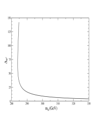
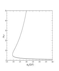
Figure 5: Fine tuning in the unconventional SUSY scenario of section 4 as a function of the Higgs mass (in GeV) for $\tan\beta=10$ and the rest of parameters as in set A (left) or as in set B (right).

This behaviour is shown in Figure 5, left plot, which is the equivalent of fig. 1, but for the unconventional scenario just introduced, with $\tan\beta=10$. We can use the soft mass $\tilde{m}$ as a parameter along the curve plotted, with $\Delta_{\mu^{2}}$ growing for increasing $\tilde{m}$. In the large-$\tilde{m}$ range of this curve (its steep upper branch) radiative corrections dominate the Higgs mass and the behaviour of the fine tuning is similar to that in the MSSM (i.e. it grows with increasing $m_{h}$). If we restrict our attention to the more interesting low-$\tilde{m}$ range (the lower branch of the curve), the contrast with the MSSM result is evident: now, the larger $m_{h}$ is, the smaller the tuning becomes and for $m_{h}\stackrel{{\scriptstyle>}}{{{}_{\sim}}}300$ one gets $\Delta_{\mu^{2}}<10$. All this is the straightforward result of having a larger tree level contribution to the Higgs mass. For the choice of parameters considered here (set A) the resulting Higgs mass is somewhat large, but we can easily choose different parameters in order to lower the Higgs mass without loosing the dramatic improvement in $\Delta_{\mu^{2}}$. This is shown on the right plot of fig. 5, which has (set B): $\mu/M=0.3$, $e_{1}=-2$, $\tilde{m}/M=0.5$, $\alpha_{t}=1$ and $\alpha_{1}\stackrel{{\scriptstyle>}}{{{}_{\sim}}}0.36$. The bi-valuedness of $\Delta_{\mu^{2}}$ is more evident in this case.

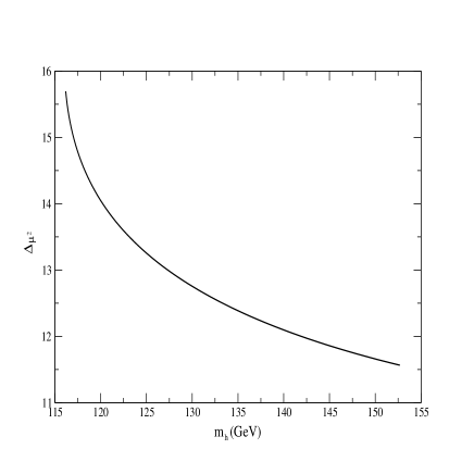
Figure 6: Fine tuning in a low-scale SUSY breaking scenario as a function of the Higgs mass (in GeV) for $\tan\beta=10$.

We plot $\Delta_{\mu^{2}}$ vs. $m_{h}$ in Fig. 6 to make even clearer the difference of behaviour with respect to the MSSM (see fig. 1). We take $\mu=330$ GeV, $\tilde{m}=550$ GeV, $e_{1}=-2$, $\alpha_{t}=1$, $l$ chosen to give $\tan\beta=10$ and instead of fixing $\tilde{m}/M$ we vary it from 0.05 to 0.8. In this way we can study the effect on the fine tuning of varying $\lambda$ when the low energy mass scales ($\mu$ and $\tilde{m}$) are kept fixed. When $\tilde{m}/M$ is small (and this implies that $\mu/M$ is also small), the unconventional corrections to quartic couplings are not very important and the Higgs mass tends to its MSSM value. As $\tilde{m}/M$ increases, the tree level Higgs mass (or $\lambda$) also grows and this makes $\Delta_{\mu^{2}}$ decrease with $m_{h}$, just the opposite of the MSSM behaviour.

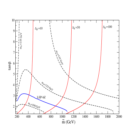
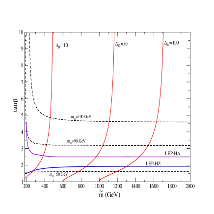
Figure 7: Fine tuning in the $(\tilde{m},\tan\beta)$ plane in a low-scale SUSY breaking scenario with parameters as in set B. Dashed lines are contour lines of constant $m_{h}$ (upper plot) or $m_{H}$ (lower plot). The LEP bound for each case is also shown.

Finally, fig. 7 is the version of Fig. 3 for this unconventional model. The values of the parameters are those of set B. We show lines of constant $\Delta_{\mu^{2}}$ in the $(\tilde{m},\tan\beta)$ plane, together with lines of constant $m_{h}$ (upper plot) and $m_{H}$ (lower plot). In each plot we also draw the experimental lower bound on the corresponding Higgs mass coming from LEP, either for Higgs-strahlung or associated production as indicated (see Appendix B for details). We find that the fine tuning is larger for smaller $\tan\beta$ and larger $\tilde{m}$, as in the MSSM, but now the overall value of $\Delta_{\mu^{2}}$ is significantly smaller. From the figure we can estimate that for soft masses $\tilde{m}^{2}\sim av^{2}$, the fine tuning in this model (say near $m_{h}=115$ GeV and $\tan\beta=3$) is $\Delta\sim 3.5a$ instead of the $\sim 20a$ we found for the MSSM. The pattern of Higgs masses is also different and restricting the fine tuning to be less than 10 does not impose an upper bound on the Higgs masses, in contrast with the MSSM case. As a result, the LEP bounds do not imply a large fine tuning: in the region with small $\tilde{m}$ and $\tan\beta$ not too close to 1, we can get simultaneously Higgs masses large enough to escape LEP detection and small fine tunings. In any case, following the line of $\Delta_{\mu^{2}}=10$ we do find an upper bound $\tilde{m}\stackrel{{\scriptstyle<}}{{{}_{\sim}}}500$ GeV, so that LHC would either find superpartners or revive an (LHC) fine tuning problem for these scenarios (although the problem would be much softer than in the MSSM).

5 Concluding remarks

1. As is well known, in the MSSM a successful electroweak breaking requires substantial fine-tuning. This fine tuning is abnormally large in the following sense: if the soft parameters have a size $m_{\rm soft}^{2}\sim av^{2}$, one expects a fine tuning of one part in $a$; but in practice it is more than 20 times larger.

2. The main reason for that is the small magnitude of the tree-level Higgs quartic coupling $\lambda_{\rm MSSM}={1\over 8}(g^{2}+g_{Y}^{2})\cos^{2}2\beta\ \simeq\ {1\over 15}\cos^{2}2\beta$. This has two effects:

   • The “natural” value for the Higgs VEV, $v^{2}\sim m_{\rm soft}^{2}/\lambda$ tends to be much larger than $m_{\rm soft}^{2}$, specially if $\tan\beta$ is not large.

   • Sizeable radiative corrections (and thus sizeable soft terms) are needed to satisfy the experimental bound on $m_{h}$, which worsens the fine tuning problem. Since $m_{h}$ increases logarithmically with $m_{\rm soft}$, the problem gets exponentially worse for increasing $m_{h}$.

   In addition, the radiative mechanism for EW breaking aggravates the problem, since it induces large coefficients for the individual contributions of certain soft terms to the effective potential.

3. As a consequence, the most efficient way of reducing the fine tuning is to consider supersymmetric models where $\lambda_{\rm tree}$ is larger than in the MSSM. [An estimate of the expected improvement in the fine tuning, using the ordinary fine tuning parameters is given in eq.(15)]

4. The latter possibility takes place naturally in scenarios in which the breaking of SUSY occurs at a low scale (not far from the TeV scale). Then, the quartic couplings get SUSYcorrections, $\delta\lambda\sim m_{\rm soft}^{2}/M^{2}$, so that $\lambda+\delta\lambda$ can be easily larger than $\lambda_{\rm MSSM}$, as desired to ameliorate the fine tuning problem. Moreover, this opens up many new possibilities for EW breaking and for a non-conventional Higgs spectrum.

5. We demonstrate this in an explicit model of low-scale SUSYstudied in a previous paper by its own sake (and not with the goal of solving the fine tuning problem). This indicates that the improvement in the fine tuning is indeed a generic feature of these scenarios.

   By modifying the parameters of the model we achieve a dramatic improvement of the fine tuning for any range of $\tan\beta$ and the Higgs mass (which can be as large as several hundred GeV if desired, but this is not necessary). It is in fact quite easy to get e.g. $\Delta<5$ (i.e. no fine tuning), in contrast with the MSSM values, $\Delta>20$ (and much larger for $m_{h}>115$ GeV and/or small $\tan\beta$).

6. In scenarios with low-scale SUSY, the interval of running of the soft parameters is small, which has further consequences:

   • EW breaking takes place at tree-level, which, as discussed in point 2), also helps in reducing the fine tuning.

   • The cross-talk (through RG running) between mass parameters in the Higgs sector and those of other sectors (squarks, gluinos, etc.) is drastically reduced. The latter can be (much) heavier than $M_{Z}$ without upsetting the naturalness of the electroweak scale. In this sense these scenarios represent an alternative to other options which try to reduce the fine tuning by postulating correlations between different parameters to implement cancellations in $M_{Z}$: here $M_{Z}$ does not even depend strongly on those parameters.

7. The previous point is also very interesting for flavour physics in two different fronts. First, in the MSSM the stringent FCNC bounds on the non-universality of the sparticle mass matrices (e.g. from the $K$-$\bar{K}$ system) could now be alleviated simply by increasing the relevant soft masses (e.g. beyond 1 TeV) with negligible effect in EW breaking. Second, as it is known, even assuming UV universality, RG evolution induces flavour violating effects which for the $\mu\rightarrow e\gamma$ process are extremely dangerous. This problem is eliminated in the context of low scale SUSY breaking, where the RG effects are minimized (for a discussion see [29]). Incidentally, the two flavour problems just mentioned can also be understood as fine tuning problems of the MSSM.

8. Finally, it is clear that, apart from scenarios with low-scale SUSY, there are other extensions of the MSSM which increase $\lambda_{\rm tree}$ and thus improve the fine tuning. An alternative, discussed in [28], is to enlarge the Higgs sector, as in the NMSSM. This framework, however, is less effective for a number of reasons. First, the simplest NMSSM model gives an extra contribution to $\lambda$ that vanishes for large $\tan\beta$, precisely the region where the MSSM fine tuning was smallest (even if still too large). Second, the conventional NMSSM with soft terms generated at very high scale has important bounds on the previous extra contribution, derived from the requirement of perturbativity. This means that the available increase in $\lambda_{\rm tree}$ (and the consequent improvement in the fine tuning) is more modest than could be thought a priori. Finally, EW breaking still occurs radiatively, which eliminates the extra bonus discussed in 6) above.

A. General formulas for fine tuning parameters

Here we consider a generic scenario where the Higgs sector consists of two $SU(2)_{L}$ doublets of opposite hypercharge, $H_{1}$ and $H_{2}$, as is the case in many supersymmetric models [30]. The most general Higgs potential for such two Higgs doublet models (2HDM) is (at tree level)

$$V = m_{1}^{2}|H_{1}|^{2}+m_{2}^{2}|H_{2}|^{2}-\left[m_{3}^{2}H_{1}\cdot H_{2}+{\rm h.c.}\right]$$ (A.1)

$$+ {1\over 2}\lambda_{1}|H_{1}|^{4}+{1\over 2}\lambda_{2}|H_{2}|^{4}+\lambda_{3}|H_{1}|^{2}|H_{2}|^{2}+\lambda_{4}|H_{1}\cdot H_{2}|^{2}$$

$$+ \left[{1\over 2}\lambda_{5}(H_{1}\cdot H_{2})^{2}+\lambda_{6}|H_{1}|^{2}H_{1}\cdot H_{2}+\lambda_{7}|H_{2}|^{2}H_{1}\cdot H_{2}+{\rm h.c.}\right]\ .$$

The minimum of this potential occurs in general at non-zero values of the neutral components of the Higgs doublets, $H_{1}^{0}$ and $H_{2}^{0}$ with $\tan\beta\equiv\langle H^{0}_{2}\rangle/\langle H^{0}_{1}\rangle$ and $\langle H^{0}_{1}\rangle=(v/\sqrt{2})\cos\beta$, $\langle H^{0}_{2}\rangle=(v/\sqrt{2})\sin\beta$. It is useful to write $V$ as a ‘SM-like’potential for $v$:

$$V(v)={1\over 2}m^{2}v^{2}+{1\over 4}\lambda v^{4}\ ,$$ (A.2)

where $\lambda$ and $m^{2}$ are functions of $\tan\beta$ and the initial parameters of the theory, $p_{\alpha}$. Explicitly

$$m^{2}=\sum_{i=1}^{3}c_{i}(\beta)m_{i}^{2}(p_{\alpha}),\;\;\;\;\;\;\vec{c}=(c^{2}_{\beta},s^{2}_{\beta},-s_{2\beta})\ ,$$ (A.3)

and

$$\lambda=\sum_{i=1}^{7}d_{i}(\beta)\lambda_{i}(p_{\alpha}),\;\;\;\;\;\;\vec{d}=({1\over 2}c^{4}_{\beta},{1\over 2}s^{4}_{\beta},s^{2}_{\beta}c^{2}_{\beta},s^{2}_{\beta}c^{2}_{\beta},s^{2}_{\beta}c^{2}_{\beta},c^{2}_{\beta}{s_{2\beta}},s^{2}_{\beta}{s_{2\beta}})\ .$$ (A.4)

Minimization of $V$ with respect to $v$ and $\beta$ implies

$$v^{2}={-m^{2}\over\lambda}\ ,$$ (A.5)

$$2\lambda\frac{\partial m^{2}}{\partial\beta}-m^{2}\frac{\partial\lambda}{\partial\beta}=0\ .$$ (A.6)

In order to evaluate the fine tuning in a generic theory of this kind, we will use the fine tuning parameters, $\Delta_{p_{\alpha}}$, introduced by Barbieri and Giudice [3]:

$${\delta M_{Z}^{2}\over M_{Z}^{2}}={\delta v^{2}\over v^{2}}=\Delta_{p_{\alpha}}{\delta p_{\alpha}\over p_{\alpha}}\ ,$$ (A.7)

where $\delta M_{Z}^{2}$ ($\delta v^{2}$) is the change induced in $M_{Z}^{2}$ ($v^{2}$) by a change $\delta p_{\alpha}$ in $p_{\alpha}$. Naturalness requires $\Delta_{p_{\alpha}}\stackrel{{\scriptstyle<}}{{{}_{\sim}}}{\cal O}(10)$.

Applying eq. (A.7) to eq. (A.5) we get, after trading $\partial m^{2}/\partial\beta$ by $\partial\lambda/\partial\beta$ using eq. (A.6),

$$\Delta_{p}=\frac{p}{m^{2}}\left[\frac{\partial m^{2}}{\partial p}+\frac{v^{2}}{2}\frac{\partial\lambda}{\partial\beta}\frac{d\beta}{dp}+v^{2}\frac{\partial\lambda}{\partial p}\right]\ .$$ (A.8)

The dependence of $\beta$ on $p$, which is not explicit in the initial potential (A.1), can be extracted from eq. (A.6) by acting on it with $d/dp$, to obtain finally

$$\Delta_{p}=-{p\over x}\left[\left(2{\partial^{2}m^{2}\over\partial\beta^{2}}+v^{2}{\partial^{2}\lambda\over\partial\beta^{2}}\right)\left({\partial\lambda\over\partial p}+{1\over v^{2}}{\partial m^{2}\over\partial p}\right)-{\partial\lambda\over\partial\beta}{\partial^{2}m^{2}\over\partial\beta\partial p}+{\partial m^{2}\over\partial\beta}{\partial^{2}\lambda\over\partial\beta\partial p}\right]\ ,$$ (A.9)

where

$$x\equiv\lambda\left(2\frac{\partial^{2}m^{2}}{\partial\beta^{2}}+v^{2}\frac{\partial^{2}\lambda}{\partial\beta^{2}}\right)-\frac{v^{2}}{2}\left(\frac{\partial\lambda}{\partial\beta}\right)^{2}\ .$$ (A.10)

[Note that the dependence of $m^{2}$ and $\lambda$ on $\beta$ is determined by eqs. (A.3, A.4).]

In many cases, equations (A.8) and (A.9) admit expansions which are useful for fine tuning estimates (although in the computations of this paper we have used the complete expressions). If there exists a fine tuning at all, there must be some cancellation between the various contributions to $m^{2}$, say ${\tt m_{i}^{2}}$, which generically implies $\partial m^{2}/\partial p={\cal O}({\tt m_{i}^{2}}/p)\gg{\cal O}(m^{2}/p)$. Then, the last two terms within the brackets in eq. (A.8) are suppressed by a factor ${\cal O}(m^{2}/{\tt m_{i}^{2}})$, and

$$\Delta_{p}\simeq\frac{p}{m^{2}}\frac{\partial m^{2}}{\partial p}=-\frac{p}{\lambda v^{2}}\frac{\partial m^{2}}{\partial p}\ .$$ (A.11)

The same result can be obtained from eq. (A.9).

Let us now consider how the previous results are modified by radiative corrections. As is well-known, the 1-loop correction to the effective Higgs potential in a supersymmetric theory (using the $\overline{\rm DR}$ renormalization scheme) is given by

$$\delta_{1}V={1\over 64\pi^{2}}\sum_{a}N_{a}M_{a}^{4}(H)\left[\log{M_{a}^{2}(H)\over Q^{2}}-{3\over 2}\right]\ ,$$ (A.12)

where $Q$ is the renormalization scale, $M_{a}^{2}(H)$ is the $H$-dependent mass eigenvalue of the particle $a$ and $N_{a}$ its multiplicity (taken negative for fermions). $\delta_{1}V$ modifies the minimization conditions as well as $m_{h}$. However, it is possible to reproduce these results by using appropriately (one-loop) corrected $m^{2}_{i}$, $\lambda_{i}$ parameters in the tree-level expressions, e.g. the minimization equations (A.5, A.6) [32]. In this way, one can still use all the previous (tree-level-like) equations (A.8–A.11) for fine tuning estimates. In particular, the dominant contribution to the fine tuning is still given by eq. (A.11) but expressed in terms of the one-loop corrected parameters.

Now, one expects $\delta_{1}m_{i}^{2}={\cal O}(Nh^{2}{\tilde{m}}^{2}/(32\pi^{2}))$, $\delta_{1}\lambda_{i}={\cal O}(Nh^{4}/(32\pi^{2}))$, where $h$ is the coupling constant of a field with multiplicity $N$ to the Higgses and ${\tilde{m}}^{2}$ is a typical soft mass. Moreover there can be a logarithmic factor $\sim\log({\tilde{m}}^{2}/m_{t}^{2})$. Clearly $\delta_{1}m_{i}^{2}$ are smaller than the typical ${\cal O}({\tilde{m}}^{2})$ tree-level contributions, so they do not affect the degree of fine tuning. On the other hand, $\delta_{1}\lambda_{i}$ can be relevant if the tree-level values are small, as it happens for instance in the MSSM (but not in models with sizeable $\lambda_{\rm tree}$, as those considered in this paper). These corrections are normally dominated by the top-stop sector with coupling $h_{t}=\sqrt{2}m_{t}/(v\sin\beta)$, which besides being ${\cal O}(1)$ has large multiplicity, $N_{L}+N_{R}=12$. If some of the Higgs self-couplings, $\lambda_{i}$, are initially large, say ${\cal O}(1)$, they can also contribute substantially to $\delta_{1}\lambda_{i}$, though the multiplicity is smaller than for the stops. However, as mentioned above, in this case $\delta_{1}\lambda_{i}\ll\lambda_{\rm tree}$ and therefore such corrections can be ignored for the fine tuning issue.

Consequently, for fine tuning estimates, we approximate the radiative corrections by the logarithmic stop contribution (more sophisticated expressions for $\delta_{1}\lambda_{i}$ can be found in [31]):

$$\delta_{1}\lambda_{2}={3h_{t}^{4}\over 8\pi^{2}}\log{M_{\rm SUSY}^{2}\over m_{t}^{2}}\ .$$ (A.13)

In particular the approximate formula given in eq. (A.11) simply gets corrected by a factor $\lambda_{\rm tree}/\lambda_{\rm 1-loop}$.

B. LEP Higgs bounds

The main Higgs production mechanism of the physical CP-even scalars ${\cal H}_{\alpha}^{0}=h^{0},H^{0}$ at LEP is $e^{+}e^{-}\rightarrow Z^{0}{\cal H}_{\alpha}^{0}$. The Higgs production cross-section is

$$\sigma_{Z{\cal H}_{\alpha}}=\xi_{{\cal H}_{\alpha}}^{2}\sigma_{Zh}^{SM}(m^{2}_{{\cal H}_{\alpha}})\ ,$$ (B.1)

where $\sigma_{Zh}^{SM}(m^{2})$ is the SM production cross-section for a Higgs with mass $m$ [33] and the prefactor $\xi_{{\cal H}_{\alpha}}$ measures the coupling $Z^{0}Z^{0}{\cal H}_{\alpha}^{0}$ relative to the SM value. In a generic 2HDM the linear combination along the breaking direction $h_{\parallel}\equiv h_{1}^{0r}\cos\beta+h_{2}^{0r}\sin\beta$ has a coupling to $ZZ$ of SM strength while the orthogonal combination $h_{\perp}\equiv h_{1}^{0r}\sin\beta-h_{2}^{0r}\cos\beta$ does not couple to $ZZ$. In the basis $\{h_{\parallel},h_{\perp}\}$ the mass eigenstates $h^{0},H^{0}$ read

$$h^{0}=\xi_{h}h_{\parallel}+\xi_{H}h_{\perp}\ ,\;\;\;\;H^{0}=\xi_{H}h_{\parallel}-\xi_{h}h_{\perp}\ ,$$ (B.2)

with $\xi_{h}^{2}+\xi_{H}^{2}=1$. That is, the coupling ${\cal H}_{\alpha}^{0}Z^{0}Z^{0}$ is proportional to the amount of $h_{\parallel}$ that enters in the composition of ${\cal H}_{\alpha}^{0}$. From the definition of $\tan\beta$ and that of the mixing angle of the two CP-even Higgs bosons $h^{0},H^{0}$:

$$h^{0} = h_{2}^{0r}\cos\alpha-h_{1}^{0r}\sin\alpha\ ,$$

$$H^{0} = h_{1}^{0r}\cos\alpha+h_{2}^{0r}\sin\alpha\ ,$$ (B.3)

we obtain the familiar expressions

$$\xi_{h}^{2}=\sin^{2}(\alpha-\beta)\ ,\;\;\;\;\xi_{H}^{2}=\cos^{2}(\alpha-\beta)\ .$$ (B.4)

In the alternative scenario considered in section 4, at tree level, the mass matrix for CP-even Higgses (in the basis $\{h_{1}^{0r},h_{2}^{0r}\}$) is

$$M^{2}_{{\cal H}_{\alpha}^{0}} = \left[\begin{array}[]{ccc}m_{\parallel}^{2}c^{2}_{\beta}+m_{\perp}^{2}s^{2}_{\beta}&&(m_{\parallel}^{2}-m_{\perp}^{2})c_{\beta}s_{\beta}\\ &&\\ (m_{\parallel}^{2}-m_{\perp}^{2})c_{\beta}s_{\beta}&&m_{\parallel}^{2}s^{2}_{\beta}+m_{\perp}^{2}c^{2}_{\beta}\end{array}\right]$$ (B.8)

$$= \left(\begin{array}[]{cc}c_{\beta}&s_{\beta}\\ &\\ s_{\beta}&-c_{\beta}\end{array}\right)\left[\begin{array}[]{cc}m_{\parallel}^{2}&0\\ &\\ 0&m_{\perp}^{2}\end{array}\right]\left(\begin{array}[]{cc}c_{\beta}&s_{\beta}\\ &\\ s_{\beta}&-c_{\beta}\end{array}\right)\ .$$ (B.18)

This implies that $h_{\parallel}$ and $h_{\perp}$ are in fact mass eigenstates and means in particular that only $h_{\parallel}$ could be produced at LEP. For some choice of parameters (like in set A, used in section 4), $h_{\parallel}$ turns out to be the heavy state, and its mass makes it kinematically inaccessible at LEP. The light state turns out to be $h_{\perp}$ and even if it is light it does not couple to $Z^{0}$ and therefore it is not produced.

At one loop the previous situation changes. Corrections to the mass matrix (B.18), the main one being

$$\delta\langle h_{2}^{0r}|M^{2}_{H_{i}^{0}}|h_{2}^{0r}\rangle={3m_{t}^{4}\over\pi^{2}v^{2}s_{\beta}^{2}}\log{M_{\rm SUSY}\over m_{t}}\ ,$$ (B.19)

induce deviations of the mass eigenstates from $h_{\parallel}$ and $h_{\perp}$, making $\xi_{h}$ and $\xi_{H}$ different from 1 and 0. Working out the expression for the one-loop corrected $\alpha$ we arrive at the simple result

$$\xi_{h}^{2}={\displaystyle{(m^{2}_{H}-m^{2}_{h_{\parallel}})c_{\beta}^{2}+(m^{2}_{h_{\perp}}-m^{2}_{h})s_{\beta}^{2}\over m^{2}_{H}-m^{2}_{h}}}\ ,$$ (B.20)

and

$$\xi_{H}^{2}={\displaystyle{(m^{2}_{H}-m^{2}_{h_{\perp}})s_{\beta}^{2}+(m^{2}_{h_{\parallel}}-m^{2}_{h})c_{\beta}^{2}\over m^{2}_{H}-m^{2}_{h}}}\ .$$ (B.21)

As discussed before, $\{h_{\parallel},h_{\perp}\}$ are the tree level mass eigenstates.

In order to implement the LEP bound in this alternative scenario, we conservatively impose that $\sigma_{Z{\cal H}_{\alpha}}$ should be smaller than $\sigma_{Zh}^{SM}(m^{2}_{h})$ evaluated at $\sqrt{s}=209$ GeV and $m_{H}=115$ GeV (the ultimate LEP bound on the SM Higgs mass). This requirement can be represented as an upper limit on $\xi_{{\cal H}_{\alpha}}^{2}$ as a function of $m_{h}$. A more refined bound (unnecessarily sophisticated for our purposes) can be found on the experimental papers [34, 35].

Another possible Higgs production mechanism is associated production $e^{+}e^{-}\rightarrow A^{0}{\cal H}_{\alpha}^{0}$, with cross section given by [33]

$$\sigma_{A{\cal H}_{\alpha}}=(1-\xi_{{\cal H}_{\alpha}}^{2})\bar{\lambda}\sigma_{Zh}^{SM}(m^{2}_{{\cal H}_{\alpha}})\ ,$$ (B.22)

where $\bar{\lambda}$ is a kinematical factor. The non observation of this process sets a limit on our model. We implement this limit by using the experimental bound on the coefficient $(1-\xi_{{\cal H}_{\alpha}}^{2})$ derived e.g in [36] as a function of $m_{{\cal H}_{\alpha}}+m_{A}$. (We are conservative in using that experimental curve, which applies strictly to the case $m_{{\cal H}_{\alpha}}\simeq m_{A}$, and in assuming $\sim 100\%$ branching ratios $A\rightarrow b\bar{b}$ and ${\cal H}_{\alpha}\rightarrow b\bar{b}$.) When $(1-\xi_{{\cal H}_{\alpha}}^{2})\simeq 1$, this limit reads $m_{{\cal H}_{\alpha}}+m_{A}\stackrel{{\scriptstyle<}}{{{}_{\sim}}}195$ GeV.

Finally, charged Higgs production ($e^{+}e^{-}\rightarrow H^{+}H^{-}$) does not give constraints in this scenario because $m_{H^{\pm}}\simeq 95$ GeV while the experimental limit is around $m_{H^{\pm}}\stackrel{{\scriptstyle<}}{{{}_{\sim}}}80$ GeV [37].

References

- [1] H. P. Nilles, Phys. Rept. 110 (1984) 1; H. E. Haber and G. L. Kane, Phys. Rept. 117 (1985) 75; S. Weinberg, “The Quantum Theory Of Fields. Vol. 3: Supersymmetry”, Cambridge, UK: Univ. Pr. (2000).
- [2] L. E. Ibáñez and G. G. Ross, Phys. Lett. B 110 (1982) 215; K. Inoue, A. Kakuto, H. Komatsu and S. Takeshita, Prog. Theor. Phys. 68 (1982) 927 [Erratum-ibid. 70 (1983) 330]; L. E. Ibáñez and C. López, Nucl. Phys. B 233 (1984) 511; L. E. Ibáñez, C. López and C. Muñoz, Nucl. Phys. B 256 (1985) 218.
- [3] R. Barbieri and G. F. Giudice, Nucl. Phys. B 306 (1988) 63.
- [4] B. de Carlos and J. A. Casas, Phys. Lett. B 309 (1993) 320 [hep-ph/9303291].
- [5] M. Olechowski and S. Pokorski, Nucl. Phys. B 404 (1993) 590 [hep-ph/9303274].
- [6] G. W. Anderson and D. J. Castaño, Phys. Lett. B 347 (1995) 300 [hep-ph/9409419]; Phys. Rev. D 52 (1995) 1693 [hep-ph/9412322]; Phys. Rev. D 53 (1996) 2403 [hep-ph/9509212].
- [7] G. W. Anderson, D. J. Castano and A. Riotto, Phys. Rev. D 55 (1997) 2950 [hep-ph/9609463].
- [8] P. Ciafaloni and A. Strumia, Nucl. Phys. B 494 (1997) 41 [hep-ph/9611204].
- [9] P. H. Chankowski, J. R. Ellis and S. Pokorski, Phys. Lett. B 423 (1998) 327 [hep-ph/9712234].
- [10] R. Barbieri and A. Strumia, Phys. Lett. B 433 (1998) 63 [hep-ph/9801353].
- [11] P. H. Chankowski, J. R. Ellis, M. Olechowski and S. Pokorski, Nucl. Phys. B 544 (1999) 39 [hep-ph/9808275].
- [12] G. L. Kane and S. F. King, Phys. Lett. B 451 (1999) 113 [hep-ph/9810374].
- [13] M. Bastero-Gil, G. L. Kane and S. F. King, Phys. Lett. B 474 (2000) 103 [hep-ph/9910506].
- [14] S. Dimopoulos and G. F. Giudice, Phys. Lett. B 357 (1995) 573 [hep-ph/9507282]; K. Agashe and M. Graesser, Nucl. Phys. B 507 (1997) 3 [hep-ph/9704206]; L. Giusti, A. Romanino and A. Strumia, Nucl. Phys. B 550 (1999) 3 [hep-ph/9811386]; J. L. Feng, K. T. Matchev and T. Moroi, Phys. Rev. Lett. 84 (2000) 2322 [hep-ph/9908309]; K. Agashe, Phys. Rev. D 61 (2000) 115006 [hep-ph/9910497]; A. Romanino and A. Strumia, Phys. Lett. B 487 (2000) 165 [hep-ph/9912301].
- [15] See e.g. the appendix of J. A. Casas, J. R. Espinosa and H. E. Haber, Nucl. Phys. B 526 (1998) 3 [hep-ph/9801365].
- [16] G. L. Kane, J. Lykken, B. D. Nelson and L. T. Wang, Phys. Lett. B 551 (2003) 146 [hep-ph/0207168].
- [17] [ALEPH, DELPHI, L3 and OPAL Collaborations], Phys. Lett. B 565 (2003) 61 [hep-ex/0306033].
- [18] J. Ellis, G. Ridolfi and F. Zwirner, Phys. Lett. B 257 (1991) 83; Phys. Lett. B 262 (1991) 477; Y. Okada, M. Yamaguchi, and T. Yanagida, Prog. Theor. Phys. 85 (1991) 1; Phys. Lett. B 262 (1991) 54; H. E. Haber and R. Hempfling, Phys. Rev. Lett. 66 (1991) 1815; R. Barbieri, M. Frigeni and M. Caravaglios, Phys. Lett. B 258 (1991) 167.
- [19] A. Brignole, J. A. Casas, J. R. Espinosa and I. Navarro, [hep-ph/0301121].
- [20] G. L. Kane, B. D. Nelson, T. T. Wang and L. T. Wang, [hep-ph/0304134].
- [21] F. Abe et al. [CDF Collaboration], Phys. Rev. Lett. 82 (1999) 271 [Erratum-ibid. 82 (1999) 2808] [hep-ex/9810029]; B. Abbott et al. [D0 Collaboration], Phys. Rev. D 60 (1999) 052001 [hep-ex/9808029].
- [22] K. Harada and N. Sakai, Prog. Theor. Phys. 67 (1982) 1877; D. R. Jones, L. Mezincescu and Y. P. Yao, Phys. Lett. B 148 (1984) 317; I. Jack and D. R. Jones, Phys. Lett. B 457 (1999) 101 [hep-ph/9903365]; L. J. Hall and L. Randall, Phys. Rev. Lett. 65 (1990) 2939; F. Borzumati, G. R. Farrar, N. Polonsky and S. Thomas, Nucl. Phys. B 555 (1999) 53 [hep-ph/9902443]; S. P. Martin, Phys. Rev. D 61 (2000) 035004 [hep-ph/9907550].
- [23] A. Brignole, F. Feruglio and F. Zwirner, Nucl. Phys. B 501 (1997) 332 [hep-ph/9703286].
- [24] N. Polonsky and S. Su, Phys. Lett. B 508 (2001) 103 [hep-ph/0010113]; Phys. Rev. D 63 (2001) 035007 [hep-ph/0006174].
- [25] A. Strumia, Phys. Lett. B 466 (1999) 107 [hep-ph/9906266].
- [26] See e.g. D. Comelli and C. Verzegnassi, Phys. Lett. B 303 (1993) 277; J. R. Espinosa and M. Quirós, Phys. Lett. B 302 (1993) 51 [hep-ph/9212305]; M. Cvetič, D. A. Demir, J. R. Espinosa, L. L. Everett and P. Langacker, Phys. Rev. D 56 (1997) 2861 [Erratum-ibid. D 58 (1998) 119905] [hep-ph/9703317]. P. Batra, A. Delgado, D. E. Kaplan and T. M. Tait, [hep-ph/0309149].
- [27] M. Drees, Int. J. Mod. Phys. A 4 (1989) 3635; J. R. Ellis, J. F. Gunion, H. E. Haber, L. Roszkowski and F. Zwirner, Phys. Rev. D 39 (1989) 844; P. Binetruy and C. A. Savoy, Phys. Lett. B 277 (1992) 453. J. R. Espinosa and M. Quirós, Phys. Lett. B 279 (1992) 92; Phys. Rev. Lett. 81 (1998) 516 [hep-ph/9804235]; G. L. Kane, C. F. Kolda and J. D. Wells, Phys. Rev. Lett. 70 (1993) 2686 [hep-ph/9210242].
- [28] M. Bastero-Gil, C. Hugonie, S. F. King, D. P. Roy and S. Vempati, Phys. Lett. B 489 (2000) 359 [hep-ph/0006198].
- [29] J. A. Casas and A. Ibarra, Nucl. Phys. B 618 (2001) 171 [hep-ph/0103065]; S. M. Barr, [hep-ph/0307372].
- [30] H. E. Haber and Y. Nir, Nucl. Phys. B 335 (1990) 363.
- [31] M. Carena, J. R. Espinosa, M. Quirós and C. E. Wagner, Phys. Lett. B 355 (1995) 209 [hep-ph/9504316]; H. E. Haber, R. Hempfling and A. H. Hoang, Z. Phys. C 75 (1997) 539 [hep-ph/9609331].
- [32] See e.g. sect. 3 in B. de Carlos and J. R. Espinosa, Nucl. Phys. B 503 (1997) 24 [hep-ph/9703212].
- [33] See e.g. M. Spira and P. M. Zerwas, [hep-ph/9803257].
- [34] A. Heister et al. [ALEPH Collaboration], Phys. Lett. B 526 (2002) 191 [hep-ex/0201014]; J. Fernandez [DELPHI Collaboration], [hep-ex/0307002]; G. Abbiendi et al. [OPAL Collaboration], Eur. Phys. J. C 27 (2003) 311 [hep-ex/0206022]; P. Achard et al. [L3 Collaboration], Phys. Lett. B 545 (2002) 30 [hep-ex/0208042].
- [35] G. Abbiendi et al. [OPAL Collaboration], Eur. Phys. J. C 18 (2001) 425 [hep-ex/0007040].
- [36] [LEP Higgs Working Group Collaboration], [hep-ex/0107030].
- [37] [LEP Higgs Working Group for Higgs boson searches Collaboration], [hep-ex/0107031].