Abstract

We study the behavior of the two plane waves configuration in the LOFF phase close to $T=0$. The study is performed by using a Landau-Ginzburg expansion up to the eighth order in the gap. The general study of the corresponding grand potential shows, under the assumption that the eighth term in the expansion is strictly positive, the existence of two tricritical lines. This allows to understand the existence of a second tricritical point for two antipodal plane waves in the LOFF phase and justifies why the transition becomes second order at zero temperature. The general analysis done in this paper can be applied to other cases.

1 Introduction

The condition for the BCS pairing is that the participating fermions should have opposite momenta. This condition is realized when the Fermi spheres of the two species are the same. However in various circumstances this does not happen. For instance, in ordinary matter, in the presence of a magnetic field the energies of the spin up and spin down electrons are different and this gives rise to a splitting of the two Fermi surfaces. In the case of quarks a mass difference between the two pairing species leads indeed to such a separation. The separation can also be produced by the condition of weak equilibrium and/or charge neutrality. All these different instances can be essentially described in terms of a difference in chemical potential (real or effective), $\delta\mu=(\mu_{u}-\mu_{d})/2$, with $\mu_{u}$ and $\mu_{d}$ the chemical potentials of the two fermions. As long as the separation is not too large the BCS pairing still arises. However increasing the separation leads to a first order phase transition to the normal phase at a point known as the Clogston-Chandrasekhar [1] limit, given by $\delta\mu=\delta\mu_{1}=\Delta_{0}/\sqrt{2}$, with $\Delta_{0}$ the BCS gap.

Already many years ago Fulde, Ferrel [2] and Larkin, Ovchinnikov [3] pointed out that close to this first order transition a different pairing mechanism could arise. In this case each of the fermions lie close to their own Fermi surface and therefore the pair has non zero momentum. This phase has been called both FFLO and LOFF in the literature. Here we will adopt the name LOFF. As a consequence of the non zero momentum of the pair translational and rotational invariances are broken. It turns out that a possibility is the formation of crystalline structures with the vertices of the cell identified by the possible momenta of the pair [3]. Correspondingly the condensate has a spatial dependence of the type

$$\Delta({\bf r})=\sum_{m=1}^{P}\Delta_{m}e^{{2i{\bf q}}_{m}\cdot{\bf r}}.$$ (1)

The case of a single plane wave has been studied both in [2] and [3]. In [3] two other cases were considered: the case of two antipodal plane waves and the one corresponding to a cube. All these studies have been performed at zero temperature, $T=0$. More recently this problem has become of interest in QCD [7] just for the reasons mentioned above, that a splitting in the Fermi energies can be produced by different quark masses and/or by weak equilibrium and charge neutrality. In [8] 23 different crystalline structures have been studied (still at $T=0$) with the conclusion that the most favorable structure would correspond to the face-centered cube, described by eight plane waves.

As far as the studies at $T\not=0$ are concerned, the phase diagram in the plane $(\delta\mu,T)$ illustrating the transition from the BCS phase to the normal phase can be found in [9]. The main result is the existence of a tricritical point, that is of a point where a first-order transition line and a second order one meet. This is easily understood since at $\delta\mu=0$ we have the usual BCS second order transition at $T_{c}\approx 0.57\Delta_{0}$, whereas at $T=0$ we have a first order transition at $\delta\mu=\Delta_{0}/\sqrt{2}$. The tricritical point, $P_{tric}$ occurs at $\delta\mu_{tric}\approx 0.61\Delta_{0}$ and $T_{tric}\approx 0.32\Delta_{0}$ [10, 11]. It turns out that this tricritical point is the end point also for any LOFF phase, in the sense that at that point also the vectors ${\bf q}_{m}$ vanish and we are back to a BCS-like situation. A careful analysis of the LOFF phase has been done in [11]. The result is that it is very likely that the favored phase close to the tricritical point is the one corresponding to two antipodal vectors, that is to a condensate

$$\Delta({\bf r})=2\Delta\cos 2{\bf q}\cdot{\bf r}.$$ (2)

Furthermore the transition from this LOFF phase to the normal one is first-order close to the tricritical point. On the other hand, in [3] it has been shown that the transition is second-order at $T=0$.

From the previous considerations we see that there are at least two problems to understand, the first one is the possible change of the favored crystalline structure from the tricritical point to zero temperature and the second one is the change in the nature of the transition in the case of the antipodal structure. A partial answer to the first problem comes from two analysis made in the two-dimensional cases [12, 13]. Essentially what these authors find is that there is a series of transitions starting from the antipodal case, close to the tricritical point, between different crystalline structures. In particular, in ref. [13] it is argued that the complexity of the crystalline structure increases going toward $T=0$.

In the present paper we will be concerned with the second problem. This has been studied in [14] using the method of quasi-classical Green’s functions [15]. The result is that at very low temperature $T\approx 0.043\Delta_{0}\approx 0.075T_{c}$ there is a further tricritical point allowing the transition from the first-order to the second order. In this paper we would like to study this problem by using the more classical approach based on the Ginzburg-Landau expansion around a second order phase transition. The complication here is that we have to expand the grand potential (or the free energy) up to the eight order in the constant $\Delta$ of eq. (2):

$$\Omega=\alpha\Delta^{2}+\frac{1}{4}\beta\Delta^{4}+\frac{1}{6}\gamma\Delta^{6}+\frac{1}{8}\delta\Delta^{8}.$$ (3)

In fact, whereas around $P_{tric}$ the $\gamma$ coefficient is positive, and the expansion up to $\Delta^{6}$ is enough to characterize the tricritical point, $\gamma$ becomes negative going down in temperature [14]. Therefore for reasons of stability of the theory a further positive term in the expansion is necessary. Unfortunately no calculation of the eighth order term exists so far, therefore we will perform our study assuming $\delta$ positive up to zero temperature and we will express our results parametrically in $\delta$ itself.

Before studying the LOFF case we will consider the general phase structure for a grand potential $\Omega$ as given in eq. (3). Since we assume $\delta$ to be strictly positive, $\Omega/\delta$ depends only on the ratio of the three parameters $\alpha$, $\beta$ and $\gamma$ to $\delta$. We will show that in this three-dimensional space there are two lines of tricritical points. The point $P_{tric}$ lies on the line $\alpha=\beta=0$, $\gamma>0$. The other line is still in the plane $\alpha=0$ but it lies on the $\gamma<0$ side and it is given by the equation $9\beta\delta-2\gamma^{2}=0$.

As we have already noticed, from ref. [14] one can argue that a second order line should exist starting from $T=0$ and ending to another tricritical point. This point is located at low temperature $T/\Delta_{0}\approx 0.043$. We will take advantage of this fact by evaluating the parameters $\alpha$, $\beta$ and $\gamma$ up to the second order in $T/\Delta_{0}$. Then one has to map the space $(\alpha,\beta,\gamma)$ on the parameter space of the theory, that is $T$, $\delta\mu$ and the vector ${\bf q}$ characterizing the antipodal state to get the result. As already anticipated we find a second tricritical point with a location depending on the value of $\delta$. We recover the results of ref. [14] for very small values of $\delta$. In particular the temperature and the $\delta\mu$ values characterizing this point vary of about 25% and 1.5% in the range $0\leq\delta\leq 1$. Therefore we confirm the results of the analysis made in [14], as long as the parameter $\delta$ is strictly positive.

We would like to point out the analysis we have made of the critical points of the grand potential given in eq. (3) is completely general and as such it can be applied to all the situations where the eighth term in the Ginzburg-Landau expansion plays a role.

In Section 2 we describe the Ginzburg-Landau expansion for the LOFF case of two antipodal plane waves. Section 3 is dedicated to the study of the critical points of the grand potential (3). In Section 4 we apply the previous considerations to the LOFF case. Conclusions are given in Section 5.

2 The Ginzburg-Landau expansion for the case of two antipodal waves

As discussed first in [3] and then in [8] (see also [5, 6]) one can derive the Ginzburg-Landau expansion for the grand potential by first expanding the gap equation in the gap parameter and then integrating over the parameter itself. All the relevant equations are given in the literature at zero temperature. The extension at finite temperature is trivial and it is made by the introduction of the Matsubara frequencies. As already said we will be concerned only with the first three coefficients $\alpha$, $\beta$ and $\gamma$ which are the ones evaluated at $T=0$ in [3] and [8], and we will assume the coefficient $\delta$ to be strictly positive. Notice that we are interested at the way in which the first order transition line coming from the tricritical point becomes second order close to zero temperature. Therefore it will be enough to evaluate the coefficients of the Landau-Ginzburg expansion close to $T=0$. For that we will perform an expansion in powers of $T/\Delta_{0}$ where $\Delta_{0}$ is the BCS gap, that is the gap evaluated at a value of $\delta\mu$ smaller than the Clogston-Chandrasekhar value, $\delta\mu_{1}=\Delta_{0}/\sqrt{2}$.

The grand potential $\Omega$ is given in the GL approximation up to the sixth order in the gap by

$$\Omega = -\frac{1}{g}\Big{(}\sum_{k,n=1}^{P}\left[\Pi({\bf q_{k}},{\bf q_{n}})\,-\,1\right]\Delta^{*}_{k}\Delta_{n}\delta_{{\bf q_{k}}-{\bf q_{n}}}$$ (4)

$$+ \frac{1}{2}\sum_{k,\ell,m,n=1}^{P}J({\bf q_{k}},{\bf q_{\ell}},{\bf q_{m}},{\bf q_{n}})\Delta^{*}_{k}\Delta_{\ell}\Delta_{m}^{*}\Delta_{n}\delta_{{\bf q_{k}}-{\bf q_{\ell}}+{\bf q_{m}}-{\bf q_{n}}}$$ (5)

$$+ \frac{1}{3}\sum_{k,\ell,m,j,i,n=1}^{P}K({\bf q_{k}},{\bf q_{\ell}},{\bf q_{m}},{\bf q_{j}},{\bf q_{i}},{\bf q_{n}})\Delta^{*}_{k}\Delta_{\ell}\Delta_{m}^{*}\Delta_{j}\Delta_{i}^{*}\Delta_{n}\delta_{{\bf q_{k}}-{\bf q_{\ell}}+{\bf q_{m}}-{\bf q_{j}}+{\bf q_{i}}-{\bf q_{n}}}\Big{)}\,,$$ (6)

where $P$ is the number of independent plane waves in the condensate and

$$\Pi({\bf q_{1}},{\bf q_{2}})=\,+\,\frac{ig\rho}{2}\int\frac{d\bf\hat{w}}{4\pi}\int_{-\delta}^{+\delta}d\xi\int_{-\infty}^{+\infty}\frac{dE}{2\pi}\prod_{i=1}^{2}\,f_{i}(E,\delta\mu,\{{\bf q}\})\ ,$$ (7)

$$J({\bf q_{1}},{\bf q_{2}},{\bf q_{3}},{\bf q_{4}})=\,+\,\frac{ig\rho}{2}\int\frac{d\bf\hat{w}}{4\pi}\int_{-\delta}^{+\delta}d\xi\int_{-\infty}^{+\infty}\frac{dE}{2\pi}\prod_{i=1}^{4}\,f_{i}(E,\delta\mu,\{{\bf q}\})\ ,$$ (8)

$$K({\bf q_{1}},{\bf q_{2}},{\bf q_{3}},{\bf q_{4}},{\bf q_{5}},{\bf q_{6}})=\,+\,\frac{ig\rho}{2}\int\frac{d\bf\hat{w}}{4\pi}\int_{-\delta}^{+\delta}d\xi\int_{-\infty}^{+\infty}\frac{dE}{2\pi}\prod_{i=1}^{6}f_{i}(E,\delta\mu,\{{\bf q}\}),$$ (9)

where, by putting ${\bf w}\,\equiv\,v_{F}\,\bf\hat{w}$,

$$f_{i}(E,\delta\mu,\{{\bf q}\})=\frac{1}{E+i\epsilon\,\text{sign}\,E-\delta\mu+(-1)^{i}[\xi-2\sum_{k=1}^{i}(-1)^{k}\bf w\cdot{\bf q_{k}}]}\leavevmode\nobreak\ .$$ (10)

Moreover the condition

$$\sum_{k=1}^{M}(-1)^{k}{\bf q_{k}}=0$$ (11)

holds, with $M=2,4,6$ respectively for $\Pi$, $J$ and $K$. Furthermore $\rho$ is the density of states at the Fermi surface given by $\rho=gp_{F}^{2}/\pi^{2}v_{F}$, with $p_{F}$ Fermi momentum, $v_{F}$ the Fermi velocity and $g$ the number of degrees of freedom. In the case of two-flavor QCD in the color superconductive phase (2SC phase) one has $g=4$, $p_{F}=\mu$ and $v_{F}=1$. If the vectors $\bf q$ define a crystalline structure they belong to the orbits of the point group of the crystal. In most of the cases considered in [8] there is a single orbit, and this is the case for two antipodal waves. Therefore we assume that

$$\Delta_{k}=\Delta_{k}^{*}=\Delta\leavevmode\nobreak\ \leavevmode\nobreak\ \leavevmode\nobreak\ \leavevmode\nobreak\ \leavevmode\nobreak\ \leavevmode\nobreak\ (\text{for\ any\ }k)\,.$$ (12)

Then we can rewrite (6) as follows (for two antipodal waves):

$$\frac{\Omega}{\rho}=\alpha\Delta^{2}+\frac{\beta}{4}\Delta^{4}+\frac{\gamma}{6}\Delta^{6}\,,$$ (13)

where

$$\alpha=2\frac{1-\Pi(q)}{g\rho},$$ (14)

$$\beta = -\frac{2}{g\rho}\sum_{k,\ell,m,n=1}^{P}J({\bf q_{k}},{\bf q_{\ell}},{\bf q_{m}},{\bf q_{n}})\delta_{{\bf q_{k}}-{\bf q_{\ell}}+{\bf q_{m}}-{\bf q_{n}}},$$ (15)

$$\gamma = -\frac{2}{g\rho}\sum_{k,\ell,m,j,i,n=1}^{P}K({\bf q_{k}},{\bf q_{\ell}},{\bf q_{m}},{\bf q_{j}},{\bf q_{i}},{\bf q_{n}})\delta_{{\bf q_{k}}-{\bf q_{\ell}}+{\bf q_{m}}-{\bf q_{j}}+{\bf q_{i}}-{\bf q_{n}}}.$$ (16)

These expressions, which are obtained in [8] for $T=0$, can be easily extended to finite temperature by transforming the integration over the energy into a sum over the Matsubara frequencies according to

$$\int dE\to 2\pi iT\sum_{n=-\infty}^{+\infty},\leavevmode\nobreak\ \leavevmode\nobreak\ \leavevmode\nobreak\ E\to i\omega_{n}=(2n+1)\pi T.$$ (17)

The way of evaluating these integrals at $T=0$ is explained in [8]. One can follow the same method and perform the sum over the Matsubara frequencies using the Polygamma functions. One can get the result in a finite form, but for our purposes is more useful a low temperature expansion (in the ratio $T/\Delta_{0}$). In fact, we will be interested in analyzing the line of second order transitions starting from $T=0$. As anticipated in the Introduction we expect this line to become first order at a temperature of about $0.04\Delta_{0}$ [14], therefore an expansion up to the order $(T/\Delta_{0})^{2}$ will be sufficient.

Notice that for any crystalline structure, the coefficient $\alpha$ depends only on a single $\bf q$ vector. Therefore it has a universal structure. In particular the second order points are determined by the equation $\alpha=0$, and the optimal choice of the vector $\bf q$ along a second order line is determined by the condition

$$\frac{\partial\alpha}{\partial{\bf q}}\Big{|}_{minimum}=0.$$ (18)

This condition determines $|\bf q|$ leaving the direction of the vector arbitrary. In particular, at $T=0$, one gets

$$qv_{F}\approx 1.2\delta\mu_{2},\leavevmode\nobreak\ \leavevmode\nobreak\ \leavevmode\nobreak\ \delta\mu_{2}\approx 0.754\Delta_{0},$$ (19)

where $\delta\mu_{2}$ is the second order transition point and $\Delta_{0}$ is the BCS gap. From this it follows that all the vectors appearing in the quantities $J$ and $K$ are of the same length, therefore due to the condition of momentum conservation, only a few configurations may appear. In the actual case of two antipodal plane waves and for the $J$ integral one has (with ${\bf q}_{a}=-{\bf q}_{b}$ and $|{\bf q}_{a}|=|{\bf q}_{b}|=q$) [3]

$$J_{0}=J({\bf q_{a}},{\bf q_{a}},{\bf q_{a}},{\bf q_{a}}),\leavevmode\nobreak\ \leavevmode\nobreak\ \leavevmode\nobreak\ \leavevmode\nobreak\ J_{1}=J({\bf q_{a}},{\bf q_{a}},{\bf q_{b}},{\bf q_{b}}).$$ (20)

It results

$$\beta=-\frac{2}{g\rho}(2J_{0}+4J_{1}).$$ (21)

In the case of $K$ we have three structures

$$K_{0}=K({\bf q_{a}},{\bf q_{a}},{\bf q_{a}},{\bf q_{a}},{\bf q_{a}},{\bf q_{a}}),\leavevmode\nobreak\ \leavevmode\nobreak\ \leavevmode\nobreak\ \leavevmode\nobreak\ \leavevmode\nobreak\ K_{1}=K({\bf q_{a}},{\bf q_{a}},{\bf q_{a}},{\bf q_{a}},{\bf q_{b}},{\bf q_{b}}),$$

$$K_{2}=K({\bf q_{a}},{\bf q_{a}},{\bf q_{b}},{\bf q_{b}},{\bf q_{b}},{\bf q_{b}}),$$ (22)

with

$$\gamma=-\frac{2}{g\rho}(2K_{0}+12K_{1}+6K_{2}).$$ (23)

We are now in the position of evaluating all the quantities of interest at the order $(T/\Delta_{0})^{2}$. About this point, one can notice that all our expressions are even in $T$ and therefore we are really neglecting terms of order $(T/\Delta_{0})^{4}$.

Introducing the re-scaled variables:

$$T\to\frac{T}{\Delta_{0}},\leavevmode\nobreak\ \leavevmode\nobreak\ \leavevmode\nobreak\ Q=qv_{F}\to\frac{Q}{\Delta_{0}},\leavevmode\nobreak\ \leavevmode\nobreak\ \leavevmode\nobreak\ \delta\mu\to\frac{\delta\mu}{\Delta_{0}},$$ (24)

we get the following results

$$\alpha(\delta\mu,Q,T)=-1+\frac{\delta\mu}{2Q}\ln{\left|\frac{Q+\delta\mu}{Q-\delta\mu}\right|}-\frac{1}{2}\ln{\frac{1}{4(Q^{2}-\delta\mu^{2})}}-\frac{\pi^{2}T^{2}}{3(\delta\mu^{2}-Q^{2})},$$ (25)

$$J_{0}(\delta\mu,Q,T)=\frac{g\rho}{8}\frac{1}{\delta\mu^{2}-Q^{2}}\left(1+\frac{\pi^{2}(3\delta\mu^{2}+Q^{2})}{3(\delta\mu^{2}-Q^{2})^{2}}T^{2}\right),$$ (26)

$$J_{1}(\delta\mu,Q,T)=\frac{g\rho}{16\delta\mu}\left[\frac{1}{Q}\ln\left|\frac{\delta\mu+Q}{\delta\mu-Q}\right|+\frac{\pi^{2}}{3\delta\mu}\left(\frac{2(2\delta\mu^{2}-Q^{2})}{(\delta\mu^{2}-Q^{2})^{2}}-\frac{1}{\delta\mu Q}\ln\left|\frac{\delta\mu+Q}{\delta\mu-Q}\right|\right)T^{2}\right],$$ (27)

$$K_{0}(\delta\mu,Q,T)=\frac{g\rho}{64}\frac{1}{(\delta\mu^{2}-Q^{2})^{3}}\left(3\delta\mu^{2}+Q^{2}+\frac{2\pi^{2}(5\delta\mu^{4}+10\delta\mu^{2}Q^{2}+Q^{4})}{(\delta\mu^{2}-Q^{2})^{2}}T^{2}\right),$$ (28)

$$K_{1}(\delta\mu,Q,T)=K_{2}(\delta\mu,Q,T)=\frac{g\rho}{64\delta\mu^{2}}\left[\frac{2\delta\mu^{2}-Q^{2}}{(\delta\mu^{2}-Q^{2})^{2}}-\frac{1}{2\delta\mu Q}\ln\left|\frac{\delta\mu+Q}{\delta\mu-Q}\right|\right.$$

$$\left.+\left(\frac{2\pi^{2}(12\delta\mu^{6}-14\delta\mu^{4}Q^{2}+11\delta\mu^{2}Q^{4}-3Q^{6})}{3\delta\mu^{2}(\delta\mu^{2}-Q^{2})^{4}}-\frac{\pi^{2}}{\delta\mu^{3}Q}\ln\left|\frac{\delta\mu+Q}{\delta\mu-Q}\right|\right)T^{2}\right].$$ (29)

We have now the expansion of the grand potential up to terms of order $\Delta^{6}$. However for the following discussion one would need also the next term in the expansion. Since this is not available we will assume it to be strictly positive and we will discuss the results as functions of the coefficient $\delta$ of this term. Therefore, our grand potential will be

$$\frac{\Omega}{\rho}=\alpha\Delta^{2}+\frac{\beta}{4}\Delta^{4}+\frac{\gamma}{6}\Delta^{6}+\frac{\delta}{8}\Delta^{8},$$ (30)

with $\alpha$, $\beta$ and $\gamma$ from the calculations of this Section and $\delta$ assumed strictly positive.

3 The general phase diagram

To study the structure of the phase space let us define a dimensionless grand potential:

$$\bar{\Omega}=\frac{\Omega}{(\delta\Delta_{0}^{6})\rho\Delta_{0}^{2}}=x\left(a+\frac{b}{4}x+\frac{c}{6}x^{2}+\frac{1}{8}x^{3}\right),$$ (31)

where

$$a=\frac{\alpha}{\delta\Delta_{0}^{6}},\leavevmode\nobreak\ \leavevmode\nobreak\ \leavevmode\nobreak\ b=\frac{\beta}{\delta\Delta_{0}^{4}},\leavevmode\nobreak\ \leavevmode\nobreak\ \leavevmode\nobreak\ c=\frac{\gamma}{\delta\Delta_{0}^{2}},$$ (32)

$\Delta_{0}$ is the BCS gap and

$$x=\left(\frac{\Delta}{\Delta}_{0}\right)^{2}.$$ (33)

The minima of the grand potential are given by the equation

$$\frac{\partial\bar{\Omega}}{\partial\Delta}=\frac{\sqrt{x}}{\Delta_{0}}(2a+bx+cx^{2}+x^{3}).$$ (34)

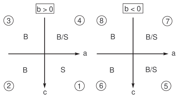
Figure 1: The octants of the space $(a,b,c)$ are illustrated in the two planes corresponding to $b>0$ (left panel) and $b<0$ (right panel). Also the phases in the various regions are indicated. $S$ is the symmetric phase, whereas $B$ is the broken one.

Notice that the structure of the minima is not changed by dividing by the parameter $\delta$ since it is assumed to be strictly positive. Therefore our phase space is a three-dimensional one. We want to determine the regions of this space corresponding to first and second order transitions. Their intersection will fix the tricritical lines. We start analyzing the roots of eq. (34) different from zero. The type of solutions with their sign is given in Table 1. Keeping in mind that we have the constraint $x>0$ for not zero roots, we can easily determine the kind of symmetry in each octant, and the result is shown in Fig. 1.

	$a$	$b$	$c$	Solutions	Phases
1	$+$	$+$	$+$	3 negative	symmetric
				1 negative, 2 complex	symmetric
2	$-$	$+$	$+$	2 negative, 1 positive	broken
				2 complex, 1 positive	broken
3	$-$	$+$	$-$	3 positive	broken
				2 complex, 1 positive	broken
4	$+$	$+$	$-$	2 positive, 1 negative	broken
				2 complex, 1 negative	symmetric
5	$+$	$-$	$+$	2 positive, 1 negative	broken
				2 complex, 1 negative	symmetric
6	$-$	$-$	$+$	2 negative, 1 positive	broken
				2 complex, 1 positive	broken
7	$-$	$-$	$-$	2 negative, 1 positive	broken
				2 complex, 1 positive	broken
8	$+$	$-$	$-$	2 positive, 1 negative	broken
				2 complex, 1 negative	symmetric

Table 1: The table shows the character of the solutions of the cubic according to the sign of the coefficients. Also shown are the phases corresponding to the various type of solutions.

In particular we see that for $a<0$ the symmetry is always broken. This is confirmed also by looking at the second derivative of $\bar{\Omega}$:

$$\Delta_{0}^{2}\frac{\partial^{2}\bar{\Omega}}{\partial\Delta^{2}}=2a+3bx+5cx^{2}+7x^{3}.$$ (35)

The point $x=0$ for $a<0$ is always a maximum, whereas for $a>0$ is a minimum, and we have to decide which is the absolute minimum. If we evaluate the second derivative at a root $x_{r}\not=0$ we find

$$\Delta_{0}^{2}\frac{\partial^{2}\bar{\Omega}}{\partial\Delta^{2}}\Big{|}_{x_{r}}=-12a-4bx_{r}-2cx_{r}^{2},$$ (36)

which is negative in the octant 1 ($a,b,c>0$). Therefore in this octant the true minimum is at $x=0$ and we are in the symmetric phase as seen from the analysis in Table 1. To decide what happens in the octants 4, 5 and 8, the ones with mixed symmetry, it is enough to look at the first order points. These are the points where, for $a\not=0$, we have a change in the symmetry. Since $a\not=0$, the only possible minimum in zero is the trivial one, and these points are determined by a change in the number of the real solutions of the cubic

$$\frac{\bar{\Omega}}{x}=a+\frac{b}{4}x+\frac{c}{6}x^{2}+\frac{1}{8}x^{3}=0,$$ (37)

as already evident from Table 1. Therefore the first order surface is made up by the points of the regions 4,5 and 8 where the discriminant of the cubic equation (37) is zero. Before discussing this point let us notice that the second order transitions are characterized by $a=0$, but not all this plane is a second order surface. Regions that correspond certainly to second order transitions is the part of the plane $a=0$ separating region 1 from region 2. In the other cases, that is 3-4, 5-6 and 7-8 one has first to discuss the region of the first order transitions.

To discuss the solutions of (37) we bring it to the normal form

$$y^{3}+py+q=0,$$ (38)

where

$$y=\frac{4c}{9}+x$$ (39)

and

$$p=2b-\frac{16}{27}c^{2},\leavevmode\nobreak\ \leavevmode\nobreak\ \leavevmode\nobreak\ q=\frac{128}{729}c^{3}-\frac{8}{9}bc+8a.$$ (40)

The discriminant of the cubic is then given by

$$D=\frac{q^{2}}{4}+\frac{p^{3}}{27}$$ (41)

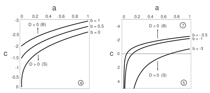
Figure 2: We show the points where $D=0$ in the region 4, $a>0,b>0,c<0$ (left panel) and in the regions 5 and 7 , $a>0,b<0$ (right panel). In the part of the octants below these curves we have $D>0$, therefore there are 2 complex and one negative root (see Table 1), and we are in the symmetric phase. By continuity the region above the curves $D=0$ belongs to the broken phase.

and we have one real and two complex solutions for $D>0$ and three real solutions for $D<0$. Therefore for $D<0$ we are typically in the broken phase. The situation is made clear in Figure 2 where we show the curves $D=0$ in the regions 4, 5 and 7 for different values of $b$.

We can now identify the tricritical lines noticing that they are necessarily at the intersection of the plane $a=0$ with the surface $D=0$ passing through the regions 4, 5 and 7. Evaluating $D$ at $a=0$ we get:

$$D|_{a=0}=\frac{2}{27}b^{2}\left(b-\frac{2}{9}c^{2}\right).$$ (42)

The line $a=0$ and $b=0$ for $c>0$ is certainly a tricritical line, since it belongs to both to the first order and the second order surfaces. As far as the line $b=2c^{2}/9$ it can be critical only for $b>0$ and $c<0$ (region 4). In fact, in this case the first order lines touch the surface $a=0$, as shown in Fig. 2, whereas in the regions 5 and 7 this does not happen (see again Fig. 2). Summarizing the tricritical lines are defined by

$$\alpha=\beta=0,\leavevmode\nobreak\ \leavevmode\nobreak\ \leavevmode\nobreak\ \leavevmode\nobreak\ \gamma>0$$ (43)

and

$$9b-2c^{2}=0,\leavevmode\nobreak\ \leavevmode\nobreak\ b>0,\leavevmode\nobreak\ \leavevmode\nobreak\ c<0.$$ (44)

The first and second order critical surfaces with their intersections are shown in the three dimensional plot of Fig. 3.

4 The second tricritical point for the two antipodal plane waves

We have now all the elements to analyze what happens in the case of two antipodal plane waves along the second order transition line starting from $T=0$. These points, as we have discussed in the previous Section are defined by the condition

$$\alpha(\delta\mu,T,Q)=0,$$ (45)

supplemented by the condition of optimality for $Q$ which amounts to require the stationarity of the grand potential $\Omega$

$$\frac{\partial\alpha(\delta\mu,T,Q)}{\partial Q}=0.$$ (46)

We can solve these two equations finding the values of $Q$ along the second order transition line and a relation between $T$ and $\delta\mu$. Of course, the result is the same as in the case of a single plane wave, since as noticed before, the expression of $\alpha$ does not depend on the number $P$ of plane waves. The transition line in the plane $(\delta\mu,T)$ is given for small values of $T$ in Fig. 4. What is different now from the case of the single plane wave is the behavior of the coefficients $\beta$ and $\gamma$. In fact, looking at Fig. 3, for the single plane wave one has a path going from $C$ ($T=0$) to $A$ (the tricritical point) staying along the second order surface, whereas in the actual case one moves from the region $\beta>0$ and $\gamma>0$ to the region $\beta>0$ and $\gamma<0$ where the second tricritical line (see eq. (44))

$$9\beta\delta-2\gamma^{2}=0$$ (47)

is met. This is shown in Fig. 5 where the behavior of $\beta$ and $\gamma$ along the second order transition line is shown as a function of the temperature. In particular we see that for $0.045\Delta_{0}\lesssim T\lesssim 0.071$, $\beta$ is positive and $\gamma$ is negative. Therefore in this region another tricritical point is found. The transition becomes first order and stays like that till the first tricritical point $A$. The location of the second tricritical point is given by equation (47) and the results are illustrated in Fig. 6. This Figure shows that the location of the tricritical point does not depend very much on the dimensionless parameter $\delta\Delta_{0}^{6}$. In fact when it varies between zero and one, the temperature of the second tricritical point varies of about 25%, whereas the value of $\delta\mu$ changes of about 1.6%. The optimal value of $Q$ stays practically constant in this range.

We can compare our results with the one obtained in [14]. In this paper it has been found, by using the method of the quasi-classical Green’s function, that the second tricritical point for the two antipodal plane waves is located at $T\approx 0.075\,T_{c}\approx 0.043\,\Delta_{0}$. By looking at Figure 6, this suggests that the actual value of $\delta$ at small temperature is rather small, but this conclusion should be confirmed by an explicit evaluation of this parameter. Also it should be noticed that the analysis made here using the Ginzburg-Landau expansion along a second order line puts this result in a more firm basis, and clarifies on a general ground the existence of a second order transition point.

5 Conclusions

In this paper we have discussed the phase structure of the LOFF phase in the configuration of two antipodal plane waves at low temperature. The interest in this study is because it is known that at $T=0$ the system undergoes a second order phase transition at a critical value of the chemical potential separation $\delta\mu$ of the two pairing species of fermions. On the other hand the transition is first order at the tricritical point $P_{tric}$. Here we clarify the reasons for this behavior as due to the existence of a second tricritical point. The most important point of the paper is that, in the case of a Ginzburg-Landau expansion up to the eighth order in the gap, the phase space is essentially three-dimensional and that two tricritical lines exist. In fact we have studied in full generality the critical points in this space, under the assumption that the eighth term in the Ginzburg-Landau expansion is strictly positive. The existence of the second tricritical point is then a simple consequence of the general structure of the phase space when the eighth order term becomes important, and it comes about since starting from $T=0$ and increasing the temperature along the second order transition line, one follows a path in the physical phase space which crosses the second tricritical line. The study made in this paper, although motivated by a particular situation (the two antipodal plane wave of the LOFF phase), is in fact much more general and it is conceivable that it can be applied to other interesting physical situations.

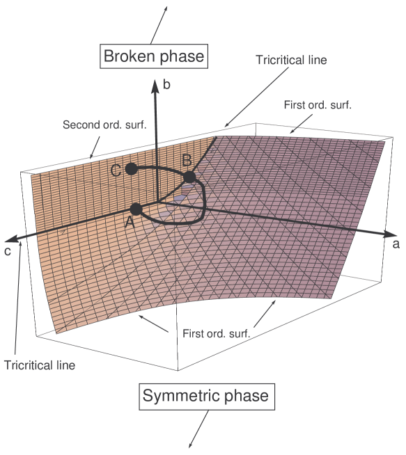
Figure 3: This three dimensional plot shows the surface of first order points in the relevant regions 4, 5 and 7 and the surface of the second order points which lies in the plane $a>0$ for $b$ and $c$ positive and in the part of the plan $b>0$ and $c<0$ delimited by the surface of the first order points. Also shown are the tricritical lines. In this figure we show also roughly the path along the critical line starting at the tricritical point (A) of the LOFF phase down to zero temperature, point C. In the path the other tricritical point B is found. The rest of the path between B and C is along the second order surface. The arrows in the boxes containing broken and symmetric phases indicate that these two phases are respectively behind and in front of the critical surfaces.

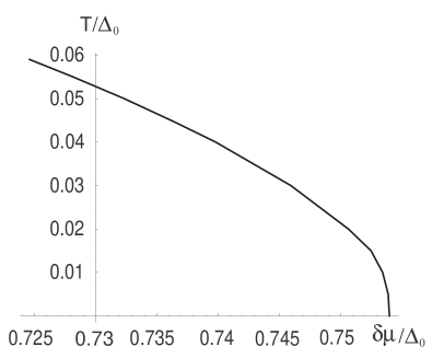
Figure 4: This figure shows the second order transition line in the plane $(\delta\mu/\Delta_{0},T/\Delta_{0})$.

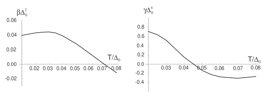
Figure 5: The dimensionless quantities $\beta\Delta_{0}^{2}$ (left panel) and $\gamma\Delta_{0}^{2}$ (right panel) vs. $T/\Delta_{0}$ along the second order transition line.

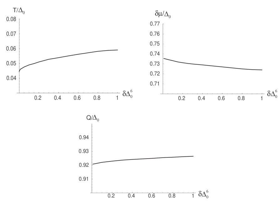
Figure 6: The figure shows the variation of the position of the second tricritical point obtained by solving eq. (47) in $T$ (left-upper panel) and $\delta\mu$ (right-upper panel). Also shown is the optimal value for the wave vector $Q$ at the tricritical point vs. $\delta$ (lower panel).

References

- [1] A.M. Clogston, Phys. Rev. Lett. 9 (1962) 266; B.S. Chandrasekhar, Appl. Phys. Lett. 1 (1962) 7.
- [2] P. Fulde and R.A. Ferrell, Phys. Rev. 135 (1964) A550.
- [3] A.I. Larkin and Y.N. Ovchinnikov, ZhETF 47 (1964) 1136 [Sov. Phys. JETP 20 (1965) 762.
- [4] H. Muther and A. Sedrakian, Phys. Rev. Lett. 88 (2002) 252503, cond-mat/0202409; W.V. Liu and F. Wilczek, Phys. Rev. Lett. 90 (2003),hep-ph/0208052; E. Gubankova, W.V. Liu and F. Wilczek, Phys. Rev. Lett. 91 (2003),hep-ph/0304016.
- [5] R. Casalbuoni and G. Nardulli, hep-ph/0305069, to be published in Rev. of Mod. Phys.
- [6] J.A. Bowers, hep-ph/0305301.
- [7] M.G. Alford, J.A. Bowers and K. Rajagopal, Phys. Rev. D63 (2001) 074016, hep-ph/0008208.
- [8] J.A. Bowers and K. Rajagopal, Phys. Rev. D66 (2002) 065002, hep-ph/0204079.
- [9] G. Sarma, J. Phys. Chem. Solids, 24 (1963) 1029; see also: D. Saint-James, G. Sarma and E.J. Thomas, Type II Superconductivity, Pergamon Press, Oxford (1969).
- [10] A.I. Buzdin and H. Kachkachi, Phys. Lett. A225 (1997) 341.
- [11] R. Combescot and C. Mora, Eur. P. J., B28 (2002) 397, cond-mat/0203031.
- [12] H. Shimahara, J. Phys. Soc. Japan 67 (1998) 736, cond-mat/9711017.
- [13] C. Morat and R. Combescot, cond-mat/0306575.
- [14] S. Matsuo, S. Higashitani, Y. Nagato and K. Nagai, J. Phys. Soc. Japan 67 (1998) 280.
- [15] M. Ashida, S. Aoyama, J. Hara and K. Nagai, Phys. Rev. B40 (1989)8673.