Dual superconductor models of color confinement

Chapter 1 Introduction

These lectures were delivered at the ECT* in Trento (Italy) in 2002 and 2003. They are addressed to physicists who wish to acquire a minimal background to understand present day attempts to model the confinement of QCD in terms of dual superconductors. The lectures focus more on the models than on attempts to derive them from QCD.

It is speculated that the QCD vacuum can be described in terms of a Landau-Ginzburg model of a dual superconductor. Particle physicists often refer to it as the Dual Abelian Higgs model. A dual superconductor is a superconductor in which the roles of the electric and magnetic fields are exchanged. Whereas, in usual superconductors, electric charges are condensed (in the form of Cooper pairs, for example), in a dual superconductor, magnetic charges are condensed. Whereas no QED magnetic charges have as yet been observed, the occurrence of color-magnetic charges in QCD, and the contention that their condensation would lead to the confinement of quarks was speculated by various authors in the early seventies, namely in the pioneering 1973 paper Nielsen and Olesen [1], the 1974 papers of Nambu [2] and Creutz [3], the 1975 papers of ’t Hooft [4], Parisi [5], Jevicki and Senjanovic [6], and the 1976 paper of Mandelstam [7]. Qualitatively, the confinement of quarks embedded in a dual superconductor can be understood as follows. The quarks carry color charge (see App.D). Consider a static quark-antiquark $\left(q\bar{q}\right)$ configuration in which the particles are separated by a distance $R$. The quark and anti-quark have opposite color-charges so that they create a static color-electric field. The field lines stem from the positively charged particle and terminate on the negatively charged particle. If the $q\bar{q}$ pair were embedded in a normal (non-superconducting) medium, the color-electric field would be described by a Coulomb potential and the energy of the system would vary as $-e^{2}/R$ where $e$ is the color-electric charge of the quarks. However, if the $q\bar{q}$ pair is embedded in a dual superconductor, the Meissner effect will attempt to eliminate the color-electric field. (Recall that, in usual superconductors, the Meissner effect expels the magnetic field.) In the presence of the color-electric charges of the quarks, Gauss’ law prevents the color-electric field from disappearing completely because the flux of the electric field must carry the color-electric charge from the quark (antiquark) to the antiquark (quark). The best the Meissner effect can do is to compress the color-electric field lines into a minimal space, thereby creating a thin flux tube which joins the quark and the antiquark in a straight line. As the distance between the quark and antiquark increases, the flux tube becomes longer but it maintains its minimal thickness. The color-electric field runs parallel to the flux tube and maintains a constant profile in the perpendicular direction. The mere geometry of the flux tube ensures that the energy increases linearly with $R$ thereby creating a linearly confining potential between the quark and the antiquark. This qualitative description hides, in fact, many problems, which relate to abelian projection (described in Chap.4), Casimir scaling, etc. As a result, attempts to model quark confinement in terms of dual superconductors are still speculative and somewhat ill defined.

The dual superconductor is described by the Landau-Ginzburg (Dual Abelian Higgs) model [8]. Because the roles of the electric and magnetic fields are exchanged in a dual superconductor, it is natural to express the lagrangian of the model in terms of a gauge potential $B^{\mu}$ associated to the dual field tensor $\bar{F}^{\mu\nu}=\partial^{\mu}B^{\nu}-\partial^{\nu}B^{\mu}$. Indeed, when the field tensor $F$ is expressed in terms of the electric and magnetic fields , as in Eq.(2.1), the corresponding expression (2.2) of the dual field tensor $\bar{F}^{\mu\nu}=\varepsilon^{\mu\nu\alpha\beta}F_{\alpha\beta}$ is obtained by the exchange $\vec{E}\rightarrow\vec{H}$ and $\vec{H}\rightarrow-\vec{E}$ of the electric and magnetic fields. (Recall that electrodynamics is usually expressed in terms of the gauge potential $A^{\mu}$ associated to the field tensor $F^{\mu\nu}=\partial^{\mu}A^{\nu}-\partial^{\nu}A^{\mu}$.) When a system is described by the gauge potential $B^{\mu}$, associated to the dual field tensor $\bar{F}$, the coupling of electric charges (such as quarks) to the gauge field $B^{\mu}$ is analogous to the problem of coupling of magnetic charges in QED to the gauge potential $A^{\mu}$. Such a coupling was formulated by Dirac in 1931 and 1948 [9] and it requires the use of a Dirac string. The Dirac theory of magnetic monopoles is reviewed in Chap.2. In Sect.2.11, it is applied to the coupling of electric charges to the gauge field $B^{\mu}$ associated to the dual field tensor $\bar{F}$.

For a system consisting of a $q\bar{q}$ pair, the Dirac string stems from the quark (or antiquark) and terminates on the antiquark (or quark). The string should not, however, be confused with the flux tube which joins the two particles in a straight line. Indeed, as explained in Sect.2.9, the Dirac string can be deformed at will by a gauge transformation. The latter does not modify the flux tube, because it is formed by the electric field and the magnetic current, both of which are gauge invariant. We refer here to the residual $U\left(1\right)$ symmetry which remains after the abelian gauge fixing (or projection), discussed in Chap.4. However, as explained in Chapt.3, there is one gauge, the so-called unitary gauge, in which the flux tube forms around the Dirac string. Calculations of flux tubes have all been performed in this gauge.

One attempt [10] to apply the dual superconductor model to a system of three quarks is discussed in Chap.5. Ultimately, this is the goal aimed at by these lectures. We would like to formulate a workable model of baryons and mesons, which would incorporate both confinement and spontaneous chiral symmetry breaking and which could be confronted to bona fide experimental data and not only to lattice data. Presently available models of hadrons incorporate either confinement or chiral symmetry, but not both. It is likely that models, such as the one described in Chap.5, will have to be implemented by an interaction between quarks and a scalar chiral field, for which there is also lattice evidence [11].

The model is inspired by (but not derived from) several observations made in lattice calculations. The first is the so-called abelian dominance, which is the observation that, in lattice calculations performed in the maximal abelian gauge, the confining string tension $\sigma$, which defines the asymptotic confining potential $\sigma R$, can be extracted from the Abelian link variables alone [12, 13],[14],[15],[16],[17],[18]. Abelian gauge fixing is discussed in Chap.4 both in the continuum and on the lattice.

The second observation, made in lattice calculations, is that the confining phase of the $SU\left(N\right)$ theory is related to the condensation of monopoles [19, 20, 21], [22, 23]. Such a statement can only be expressed in terms of an abelian gauge projection. The condensation of monopoles and confinement are found to disappear at the same temperature and it does not depend on the chosen abelian projection [25, 22]. However, confinement may well depend on the choice of the abelian gauge. In the abelian Polyakov gauge, for example, monopole condensation is observed but not confinement [26]. In Chap.4, we show how monopoles can be formed in the process of abelian projection. It is often difficult to assess the reliability and the relevance of lattice data. For example, on the lattice, even the free $U\left(1\right)$ gauge theory displays a confining phase in which magnetic monopoles are condensed [27, 28]. This confining phase disappears in the continuum limit [29] as it should, since a $U\left(1\right)$ gauge theory describes a system of free photons. However, non-abelian gauge theory is better behaved than $U\left(1\right)$ gauge theory (it is free of Landau poles) and lattice calculations point to the fact that, in the non-abelian theory, the confining phase, detected by the area law of a Wilson loop, survives even in the continuum limit.

The third observation, which favors, although perhaps not exclusively, the dual superconductor model, is the lattice measurement of the electric field and the magnetic current, which form the flux tube joining two equal and opposite static color-charges, in the maximal abelian gauge [30],[35], [31, 32, 33],[34]. They are nicely fitted by the flux tube calculated with the Landau-Ginzburg (Abelian Higgs) model, as discussed in Sect.3.4.

The model is, however, easily criticized and it has obvious failures. For example, it confines color charges, in particular quarks, which form the fundamental representation of the $SU\left(N\right)$ group and therefore carry non-vanishing color-charge. However, it does not confine every color source in the adjoint representation: for example, it would not confine abelian gluons. (Color charges of quarks and gluons are listed in App.D.) Because it is expressed in an abelian gauge, the model also predicts the existence of particles, with masses the order of $1-2\;GeV$, which are not color singlets.

In addition, there is lattice evidence for competing scenarios of color confinement, which involve the use of the maximal center gauge and center projection, described in Sect.4.3. They are usefully reviewed in the 1998 and 2003 papers of Greensite [36, 37]. They account for the full asymptotic string tension as well as Casimir scaling. In fact, both the monopole and center vortex mechanisms of the confinement are supported by the results of lattice simulations. They are related in the sense that the main part of the monopole trajectories lie on center projected vortices [38], [39]. We do not describe the center-vortex model of confinement in these lectures because it does not, as yet, lead to a classical model, such as the Landau-Ginzburg (Abelian Higgs) model. Instead, it describes confinement in terms of (quasi) randomly distributed magnetic fluxes in the vacuum. It is however, numerically simpler on the lattice and flux tubes formed by both static $q\bar{q}$ and $2q2\bar{q}$ have been computed [40]. Further scenarios, such as the Gribov coulomb gauge scenario developed by Zwanziger, Cucchieri [41, 42] and Swanson [43], and the gluon chain model of Greensite and Thorn [44, 45] are not covered by these lectures.

The relevant mathematical identities are listed in the appendices.

Chapter 2 The symmetry of electromagnetism with respect to electric and magnetic charges

The possible existence of magnetic charges and the corresponding electromagnetic theory was investigated by Dirac in 1931 and 1948 [46, 9]. The reading of his 1948 paper is certainly recommended. A useful introduction to the electromagnetic properties of magnetic monopoles can be found in Sect.6.12 and 6.13 of Jackson’s Classical Electrodynamics [47]. The Dirac theory of magnetic monopoles, which is briefly sketched in this chapter, will be incorporated into the Landau-Ginzburg model of a dual superconductor, in order to couple electric charges, which ultimately become confined. This will be done in Chapt.3.

2.1 The symmetry between electric and magnetic charges at the level of the Maxwell equations

”The field equations of electrodynamics are symmetrical between electric and magnetic forces. The symmetry between electricity and magnetism is, however, disturbed by the fact that a single electric charge may occur on a particle, while a single magnetic pole has not been observed on a particle. In the present paper a theory will be developed in which a single magnetic pole can occur on a particle, and the dissymmetry between electricity and magnetism will consist only in the smallest pole which can occur, being much greater than the smallest charge.” This is how Dirac begins his 1948 paper [9].

The electric and magnetic fields $\vec{E}$ and $\vec{H}$ can be expressed as components of the field tensor $F^{\mu\nu}$:

$$F^{\mu\nu}=\left(\begin{array}[]{cccc}0&-E_{x}&-E_{y}&-E_{z}\\ E_{x}&0&-H_{z}&H_{y}\\ E_{y}&H_{z}&0&-H_{x}\\ E_{z}&-H_{y}&H_{x}&0\end{array}\right)$$ (2.1)

They may equally well be expressed as the components of the dual field tensor $\bar{F}^{\mu\nu}$:

$$\overline{F}^{\mu\nu}=\frac{1}{2}\varepsilon^{\mu\nu\alpha\beta}F_{\alpha\beta}=\left(\begin{array}[]{cccc}0&-H_{x}&-H_{y}&-H_{z}\\ H_{x}&0&E_{z}&-E_{y}\\ H_{y}&-E_{z}&0&E_{x}\\ H_{z}&E_{y}&-E_{x}&0\end{array}\right)$$ (2.2)

where $\varepsilon^{\mu\nu\alpha\beta}$ is the antisymmetric tensor with $\varepsilon^{0123}=1$. Thus, the cartesian components of the electric and magnetic fields can be expressed as components of either the field tensor $F$ or its dual $\bar{F}$:

$$E^{i}=-F^{0i}=\frac{1}{2}\varepsilon^{0ijk}\bar{F}_{jk}\;\;\;\;\;\;\;\;H^{i}=-\bar{F}^{0i}=-\frac{1}{2}\varepsilon^{0ijk}F_{jk}$$ (2.3)

The appendix A summarizes the properties of vectors, tensors and their dual forms. In the duality transformation $F\rightarrow\overline{F}$, the electric and magnetic fields are interchanged as follows:

$$F\rightarrow\overline{F}\;\;\;\;\;\;\vec{E}\rightarrow\vec{H}\;\;\;\;\;\vec{H}\rightarrow-\vec{E}$$ (2.4)

The electric charge $\rho$ and the electric current $\vec{j}$ are components of the 4-vector $j^{\mu}$:

$$j^{\mu}=\left(\rho,\vec{j}\right)$$ (2.5)

Similarly, the magnetic charge $\rho_{mag}$ and the magnetic current $\vec{j}_{mag}$ are components of the 4-vector $j_{mag}^{\mu}$:

$$j_{mag}^{\mu}=\left(\rho_{mag},\vec{j}_{mag}\right)$$ (2.6)

At the level the Maxwell equations, there is a complete symmetry between electric and magnetic currents and the coexistence of electric and magnetic charges does not raise problems. The equations of motion for the electric and magnetic fields $\vec{E}$ and $\vec{H}$ are the Maxwell equations which may be cast into the symmetric form:

$$\partial_{\nu}F^{\nu\mu}=j^{\mu}\;\;\;\;\;\;\;\;\;\;\partial_{\nu}\overline{F}^{\nu\mu}=j_{mag}^{\mu}$$ (2.7)

It is this symmetry which impressed Dirac, who probably found it upsetting that the usual Maxwell equations are obtained by setting the magnetic current $j_{mag}^{\mu}$ to zero. The Maxwell equations can also be expressed in terms of the electric and magnetic fields $\vec{E}$ and $\vec{H}$. Indeed, if we use the definitions (2.1) and (2.2), the Maxwell equations (2.7) read:

$$\partial_{\nu}F^{\nu\mu}=j^{\mu}\;\;\rightarrow\;\;\vec{\nabla}\cdot\vec{E}=\rho\;\;\;\;\;\;-\partial_{t}\vec{E}+\vec{\nabla}\times\vec{H}=\vec{j}$$

$$\partial_{\nu}\overline{F}^{\nu\mu}=j_{mag}^{\mu}\;\;\rightarrow\;\;\vec{\nabla}\cdot\vec{H}=\rho_{mag}\;\;\;\;\;\;\;-\partial_{t}\vec{H}-\vec{\nabla}\times\vec{E}=\vec{j}_{mag}$$ (2.8)

2.2 Electromagnetism expressed in terms of the gauge field $A^{\mu}$ associated to the field tensor $F^{\mu\nu}$

So far so good. Problems however begin to appear when we attempt to express the theory in terms of vector potentials, alias gauge potentials. Why should we? In the very words of Dirac [9]: ”To get a theory which can be transferred to quantum mechanics, we need to put the equations of motion into a form of an action principle, and for this purpose we require the electromagnetic potentials.”

This is usually done by expressing the field tensor $F^{\mu\nu}$ in terms of a vector potential $A^{\mu}=\left(\phi,\vec{A}\right)$:

$$F^{\mu\nu}=\partial^{\mu}A^{\nu}-\partial^{\nu}A^{\mu}\;\;\;\;\;\;\;\vec{E}=-\partial_{t}\vec{A}-\vec{\nabla}\phi\;\;\;\;\;\;\;\vec{H}=\vec{\nabla}\times\vec{A}$$ (2.9)

However, this expression leads to the identity $\partial_{\nu}\overline{F}^{\nu\mu}=0$ which contradicts the second Maxwell equation $\partial_{\nu}\overline{F}^{\nu\mu}=j_{mag}^{\mu}$. The expression $F=\partial\wedge A$ therefore precludes the existence of magnetic currents and charges. In electromagnetic theory, this is a bonus which comes for free since no magnetic charges have ever been observed. Dirac, however, was apparently more seduced by symmetry than by this experimental observation.

Let us begin to use the compact notation, defined in App.A, and in which $\partial\wedge A$ represents the antisymmetric tensor $\left(\partial\wedge A\right)^{\mu\nu}=\partial^{\mu}A^{\nu}-\partial^{\nu}A^{\mu}$. The reader is earnestly urged to familiarize himself with this notation by checking the formulas given in the appendix A, lest he become irretrievably entangled in endless and treacherous strings of indices.

Dirac proposed to modify the expression $F=\partial\wedge A$ by adding a term $-\bar{G}$:

$$F=\partial\wedge A-\bar{G}\;\;\;\;\;\;\bar{F}=\overline{\partial\wedge A}+G$$ (2.10)

where $G^{\mu\nu}=-G^{\nu\mu}$ is an antisymmetric tensor field. The latter satisfies the equation:

$$\partial\cdot G=j_{mag}$$ (2.11)

The field tensor $F^{\mu\nu}$ then satisfies both Maxwell equations, namely: $\partial\cdot F=j$ and $\partial\cdot\bar{F}=j_{mag}$. In the expressions above, the bar above a tensor denotes the dual tensor. For example, $\bar{G}_{\mu\nu}=\frac{1}{2}\varepsilon_{\mu\nu\alpha\beta}G^{\alpha\beta}$ (see App.A). For reasons which will become apparent in Sect. 2.5, we shall refer to the antisymmetric tensor $G_{\mu\nu}$ as a Dirac string term.

The string term $G_{\mu\nu}$ is not a dynamical variable. It simply serves to couple the magnetic current $j_{mag}^{\mu}$ to the system. It acts as a source term. Note that both $G$ and the equation $\partial\cdot G=j_{mag}$ are independent of the gauge potential $A^{\mu}$.

An equation for $A^{\mu}$ is provided by the Maxwell equation $\partial\cdot F=j$. When the field tensor $F$ has the form (2.10), the equation reads:

$$\partial\cdot\left(\partial\wedge A\right)-\partial\cdot\bar{G}=j$$ (2.12)

The Maxwell equation (2.12) may be obtained from an action principle. Indeed, since the string term $G$ does not depend on the gauge field $A$, the variation of the action:

$$I_{j,j_{mag}}\left(A\right)=\int d^{4}x\left(-\frac{1}{2}F^{2}-j\cdot A\right)=\int d^{4}x\left(-\frac{1}{2}\left(\left(\partial\wedge A\right)-\bar{G}\right)^{2}-j\cdot A\right)$$ (2.13)

with respect to the gauge field $A^{\mu}$, leads to the equation (2.12). The action (2.13) is invariant with respect to the gauge transformation $A\rightarrow A+\left(\partial\alpha\right)$ provided that $\partial\cdot j=0$.

The source term $G$ has to satisfy two conditions. The first is the equation $\partial\cdot G=j_{mag}$. The second is that $\partial\cdot\bar{G}\neq 0.$ If the second condition is not satisfied, the magnetic current decouples from the system. This is the reason why $G$ cannot simply be expressed as $G=\partial\wedge B$, in terms of another gauge potential $B^{\mu}$. String solutions (see Sect.2.4) of the equation $\partial\cdot G=j_{mag}$ are constructed in order to satisfy the condition $\partial\cdot\bar{G}\neq 0$.

The string term $G^{\mu\nu}$ can be expressed in terms of two vectors, which we call $\vec{E}_{st}$ and $\vec{H}_{st}$:

$$\vec{H}_{st}^{i}=-G^{0i}=\frac{1}{2}\varepsilon^{0ijk}\bar{G}_{jk}=\;\;\;\;\;\;\vec{E}_{st}^{i}=-\bar{G}^{0i}=-\frac{1}{2}\varepsilon^{0ijk}G_{jk}$$ (2.14)

The equation $\partial\cdot\bar{F}=\partial\cdot G=j_{mag}$ then translates to:

$$\vec{\nabla}\cdot\vec{H}^{st}=\rho_{mag}\;\;\;\;\;\;-\partial_{t}\vec{H}^{st}+\vec{\nabla}\times\vec{E}^{st}=\vec{j}_{mag}$$ (2.15)

Let us express the electric and magnetic fields $\vec{E}$ and $\vec{H}$ in terms of the vector potential and the string term. We define:

$$A^{\mu}=\left(\phi,\vec{A}\right)$$ (2.16)

When the field tensor $F$ has the form (2.10), the electric and magnetic fields can be obtained from (2.3), with the result:

$$\vec{E}=-\partial_{t}\vec{A}-\vec{\nabla}\phi+\vec{E}_{st}\;\;\;\;\;\;\vec{H}=\vec{\nabla}\times\vec{A}+\vec{H}_{st}$$ (2.17)

and we have:

$$-\frac{1}{2}F^{2}=-\frac{1}{2}\left(\partial\wedge A-\bar{G}\right)^{2}=\frac{1}{2}\left(-\partial_{t}\vec{A}-\vec{\nabla}\chi-\vec{E}_{st}\right)^{2}-\frac{1}{2}\left(\vec{\nabla}\times\vec{A}+\vec{H}_{st}\right)^{2}$$ (2.18)

• Exercise: Consider the following expression of the field tensor $F$ :

  $$F=\partial\wedge A-\overline{\partial\wedge B}$$ (2.19)

  in terms of two potentials $A^{\mu}$ and $B^{\mu}$. Show that $F$ will satisfy the Maxwell equations $\partial\cdot F=j$ and $\partial\cdot\bar{F}=j_{mag}$ provided that the two potentials $A$ and $B$ satisfy the equations:

  $$\partial\cdot\left(\partial\wedge A\right)=j\;\;\;\;\;\;\partial\cdot\left(\partial\wedge B\right)=j_{mag}$$ (2.20)

  Check that the variation of the action:

  $$I_{j,j_{mag}}\left(A,B\right)=\int d^{4}x\left(-\frac{1}{2}F^{2}-j\cdot A+j_{mag}\cdot B\right)$$ (2.21)

  with respect to $A$ and $B$ leads to the correct Maxwell equations. What is wrong with this suggestion? A possible expression of the field tensor in terms of two potentials is given in a beautiful 1971 paper of Zwanziger [48] (see Sect.3.11).

2.3 The current and world line
of a charged particle.

When we describe the trajectory of a point particle in terms of a time-dependent position $\vec{R}\left(t\right)$, the Lorentz covariance is not explicit because $t$ and $\vec{R}$ are different components of a Lorentz 4-vector. The function $\vec{R}\left(t\right)$ describes the trajectory in 3-dimensional euclidean space. Lorentz covariance can be made explicit if we embed the trajectory in a 4-dimensional Minkowski space, where it is described by a world line $Z^{\mu}\left(\tau\right)$, which is a 4-vector parametrized by a scalar parameter $\tau$. The parameter $\tau$ may, but needs not, be chosen to be the proper-time of the particle. This is how Dirac describes trajectories of magnetic monopoles in his 1948 paper and much of the subsequent work is cast in this language, which we briefly sketch below.

Let $Z^{\mu}\left(\tau\right)$ be the world line of a particle in Minkowski space. A point $\tau$ on the world line $Z^{\mu}\left(\tau\right)=\left(T\left(\tau\right),\vec{R}\left(\tau\right)\right)$ indicates the position $\vec{R}\left(\tau\right)$ of the particle at the time $T\left(\tau\right),$as illustrated in Fig2.1. The current $j^{\mu}\left(x\right)$ produced by a point particle with a magnetic charge $g$ can be written in the form of a line integral:

$$j^{\mu}\left(x\right)=g\int_{L}dZ^{\mu}\delta^{4}\left(x-Z\right)$$ (2.22)

along the world line of the particle. A more explicit form of the current is:

$$j^{\mu}\left(x\right)=g\int_{\tau_{0}}^{\tau_{1}}d\tau\frac{dZ^{\mu}}{d\tau}\delta^{4}\left(x-Z\left(\tau\right)\right)$$ (2.23)

where $\tau_{0}$ and $\tau_{1}$ denote the extremities of the world line, which can, but need not, extend to infinity.

Figure 2.1: The world line of a particle. For any value of $\tau$, the 4-vector $Z^{\mu}\left(\tau\right)$ indicates the position $\vec{R}\left(\tau\right)$ of the particle at the time $T\left(\tau\right)$.

In order to exhibit the content of the current (2.23), we express it in terms of a density $\rho$ and a current $\vec{j}$:

$$j^{\mu}=\left(\rho,\vec{j}\right)$$ (2.24)

Let $x^{\mu}=\left(t,\vec{r}\right)$. The current (2.23), at the position $\vec{r}$ and at the time $t$, has the more explicit form:

$$j^{\mu}\left(t,\vec{r}\right)=g\int_{\tau_{0}}^{\tau_{1}}d\tau\frac{dZ^{\mu}}{d\tau}\delta\left(t-T\left(\tau\right)\right)\delta_{3}\left(\vec{r}-\vec{R}\left(\tau\right)\right)$$ (2.25)

The expression (2.23) of the current is independent of the parametrization $Z^{\mu}\left(\tau\right)$ which is chosen to describe the world line. We can choose $\tau=T$. The density $\rho\left(t,\vec{r}\right)$ is then:

$$\rho\left(t,\vec{r}\right)=j^{0}\left(t,\vec{r}\right)=g\int_{\tau_{0}}^{\tau_{1}}d\tau\frac{dT}{d\tau}\delta\left(t-T\left(\tau\right)\right)\delta\left(\vec{r}-\vec{R}\left(\tau\right)\right)$$

$$=g\int_{\tau_{0}}^{\tau_{1}}d\tau\delta\left(t-\tau\right)\delta\left(\vec{r}-\vec{R}\left(\tau\right)\right)=g\delta\left(\vec{r}-\vec{R}\left(t\right)\right)$$ (2.26)

and the current $\vec{j}\left(t,\vec{r}\right)$ is:

$$\vec{j}\left(t,\vec{r}\right)=g\int_{\tau_{0}}^{\tau_{1}}d\tau\frac{d\vec{R}}{d\tau}\delta\left(t-\tau\right)\delta\left(\vec{r}-\vec{R}\left(\tau\right)\right)=g\frac{d\vec{R}}{dt}\delta\left(\vec{r}-\vec{R}\left(t\right)\right)$$ (2.27)

The expressions (2.26) and (2.27) are the familiar expressions of the density and current produced by a point particle with magnetic charge $g$.

2.4 The world sheet swept out by a Dirac string in Minkowski space

The Dirac string, which is added to the field tensor $F^{\mu\nu}$ in the expression (2.10), is an antisymmetric tensor $G^{\mu\nu}\left(x\right)$ which satisfies the equation:

$$\partial\cdot G=j$$ (2.28)

As stated above, not any solution of this equation will do. For example, if we attempted to express the string term in terms of a potential $B^{\mu}$ by writing, for example, $G=\partial\wedge B$, we would have $\partial\cdot\bar{G}=0$ and the string term would decouple from the action (2.13). For this reason, string solutions of the equation $\partial\cdot G=j_{mag}$ have been proposed.

The string solution can be expressed as a surface integral over a world-sheet $Z^{\mu}\left(\tau,s\right)$:

$$G^{\mu\nu}\left(x\right)=g\int d\tau ds\;\frac{\partial\left(Z_{\mu},Z_{\nu}\right)}{\partial\left(s,\tau\right)}\delta^{4}\left(x-Z\right)$$ (2.29)

The world sheet $Z^{\mu}\left(\tau,s\right)$ is parametrized by two scalar parameters $\tau$ and $s$ and:

$$\frac{\partial\left(Z_{\mu},Z_{\nu}\right)}{\partial\left(s,\tau\right)}=\frac{\partial Z_{\mu}}{\partial s}\frac{\partial Z_{\nu}}{\partial\tau}-\frac{\partial Z_{\mu}}{\partial\tau}\frac{\partial Z_{\nu}}{\partial s}$$ (2.30)

is the Jacobian of the parametrization. A point $\left(\tau,s\right)$ on the world sheet $Z^{\mu}\left(\tau,s\right)$ indicates the position $\vec{R}\left(\tau,s\right)$ at the time $T\left(\tau,s\right)$ of a particle on the world sheet. The expression (2.29) for the string $G$ is independent of the parametrization of the world sheet $Z^{\mu}\left(\tau,s\right)$ and it can be written in a compact form as a surface integral over the world sheet $Z$:

$$G_{\mu\nu}\left(x\right)=g\int_{S}d\sigma_{\mu\nu}\;\delta\left(x-Z\right)$$ (2.31)

The surface element is:

$$d\sigma_{\mu\nu}=d\tau ds\frac{\partial\left(Z_{\mu},Z_{\nu}\right)}{\partial\left(s,\tau\right)}=d\tau ds\left(\frac{\partial Z_{\mu}}{\partial s}\frac{\partial Z_{\nu}}{\partial\tau}-\frac{\partial Z_{\mu}}{\partial\tau}\frac{\partial Z_{\nu}}{\partial s}\right)$$ (2.32)

Figure 2.2: The world sheet $Z^{\mu}\left(s,\tau\right)$ swept out by a Dirac string, which stems from a particle with magnetic charge $g$ and terminates on a particle with magnetic charge $-g$. The world line of the positively charged particle is the segment joining the points $\left(s_{0},\tau_{0}\right)$ and $\left(s_{0},\tau_{1}\right)$. The world line of the negatively charged particle is the joins the points $\left(s_{1},\tau_{0}\right)$ and $\left(s_{1},\tau_{1}\right)$.

Figure 2.2 is an illustration of the world sheet which is swept out by a Dirac string which stems from a particle with magnetic charge $g$ and terminates on a particle with magnetic charge $-g$. The word line of the positively charged particle is the border of the world sheet extending from the point $\left(s_{0},\tau_{0}\right)$ to the point $\left(s_{0},\tau_{1}\right)$. The world line of the negatively charged particle is the border of the world sheet extending from the point $\left(s_{1},\tau_{0}\right)$ to the point $\left(s_{1},\tau_{1}\right)$. For any value of $\tau$, we can view the string as a line on the world sheet, which stems from the point $\left(s_{0},\tau\right)$ on the world line of the positively charged particle to the point $\left(s_{1},\tau\right)$ of the world line of the negatively charged particle (see Fig.2.1). Often authors choose to work with a world sheet with a minimal surface. This is equivalent to the use of straight line Dirac strings. An observable, which is independent of the shape of the Dirac string, is independent of the shape of the surface which defines the world sheet. If the system is composed of a single magnetic monopole, that is, of a single particle with magnetic charge $g$, then the attached string extends to infinity. The corresponding world sheet has $s_{1}\rightarrow\infty$ and it becomes an infinite surface.

Let us check that the string form (2.29) satisfies the equation $\partial\cdot G=j$:

$$\partial_{\alpha}G^{\alpha\mu}\left(x\right)=g\int_{S}d\tau ds\;\left(\frac{\partial Z^{\alpha}}{\partial s}\frac{\partial Z^{\mu}}{\partial\tau}-\frac{\partial Z^{\alpha}}{\partial\tau}\frac{\partial Z^{\mu}}{\partial s}\right)\frac{\partial}{\partial x^{\alpha}}\delta\left(x-Z\right)$$

$$=-g\int_{S}d\tau ds\;\;\left(\frac{\partial Z^{\alpha}}{\partial s}\frac{\partial Z^{\mu}}{\partial\tau}-\frac{\partial Z^{\alpha}}{\partial\tau}\frac{\partial Z^{\mu}}{\partial s}\right)\frac{\partial}{\partial Z^{\alpha}}\delta\left(x-Z\right)$$ (2.33)

We have:

$$\frac{\partial}{\partial\tau}\delta\left(x-Z\right)=\frac{\partial Z^{\alpha}}{\partial\tau}\frac{\partial}{\partial Z^{\alpha}}\delta\left(x-Z\right)$$ (2.34)

and a similar expression holds for $\frac{\partial}{\partial s}\delta\left(x-Z\right)$. We obtain thus:

$$\partial_{\alpha}G^{\alpha\mu}\left(x\right)=-g\int_{S}d\tau ds\;\left(\frac{\partial Z^{\mu}}{\partial\tau}\frac{\partial}{\partial s}\delta\left(x-Z\right)-\frac{\partial Z^{\mu}}{\partial s}\frac{\partial}{\partial\tau}\delta\left(x-Z\right)\right)$$ (2.35)

We can use Stoke’s theorem which states that, for any two functions $U\left(\tau,s\right)$ and $V\left(\tau,s\right)$, defined on the world sheet, we have:

$$\int_{S}\left(\frac{\partial U}{\partial\tau}\frac{\partial V}{\partial s}-\frac{\partial U}{\partial s}\frac{\partial V}{\partial\tau}\right)=\oint_{C}U\left(\frac{\partial V}{\partial s}ds+\frac{\partial V}{\partial\tau}d\tau\right)$$ (2.36)

where the line integral is taken along the closed line $C$ which borders the surface $S$. A more compact form of Stoke’s theorem is:

$$\int_{S}\frac{\partial\left(U,V\right)}{\partial\left(\tau,s\right)}=\oint_{C}UdV$$ (2.37)

We apply the theorem to the functions $U=\delta^{4}\left(x-Z\right)$ and $V=Z^{\mu}$ so as to obtain:

$$\partial_{\alpha}G^{\alpha\mu}\left(x\right)=g\oint_{C}\delta\left(x-Z\right)\left(\frac{\partial Z^{\mu}}{\partial\tau}d\tau+\frac{\partial Z^{\mu}}{\partial s}ds\right)=g\oint_{C}dZ^{\mu}\delta\left(x-Z\right)$$ (2.38)

We can choose, for example, the world sheet to be such that the path $C$ begins at the point $\left(s_{0},\tau_{0}\right)$ and passes successively through the points $\left(s_{0},\tau_{1}\right)$, $\left(s_{1},\tau_{1}\right)$, $\left(s_{1},\tau_{0}\right)$ before returning to the point $\left(s_{0},\tau_{0}\right)$. Then if the world line of the charged particle begins at $\left(s_{0},\tau_{0}\right)$ and ends at $\left(s_{0},\tau_{1}\right)$, the other points being at infinity, the expression (2.38) reduces to:

$$\partial_{\alpha}G^{\alpha\mu}\left(x\right)=g\int_{\tau_{0}}^{\tau_{1}}d\tau\frac{dZ^{\mu}}{d\tau}\delta^{4}\left(x-Z\left(\tau\right)\right)$$ (2.39)

which, in view of (2.23), is the current $j^{\mu}\left(x\right)$ produced by the magnetically charged particle.

2.5 The Dirac string joining equal and opposite magnetic charges

The string term $G^{\mu\nu}\left(x\right)$ can be expressed in terms of the two vectors $\vec{H}_{st}$ and $\vec{E}_{st}$ defined in (2.14). We can use (2.29) to obtain an explicit expression for these vectors. Thus:

$$H_{st}^{i}\left(t,\vec{r}\right)=G^{i0}\left(t,\vec{r}\right)=g\int_{S}d\tau ds\delta\left(t-T\right)\delta_{3}\left(\vec{r}-\vec{R}\right)\left(\frac{\partial\vec{R}_{i}}{\partial s}\frac{\partial T}{\partial\tau}-\frac{\partial\vec{R}_{i}}{\partial\tau}\frac{\partial T}{\partial s}\right)$$

For a given value of $s$, we can choose $\tau=T\left(\tau,s\right)$ in which case we have $\frac{\partial T}{\partial\tau}=1$ and $\frac{\delta\tau}{\delta s}=0$. The string term $\vec{H}_{st}$ reduces to:

$$\vec{H}_{st}\left(t,\vec{r}\right)=g\int_{L}ds\frac{\partial\vec{R}}{\partial s}\delta\left(\vec{r}-\vec{R}\left(t\right)\right)=g\int_{L}d\vec{R}\delta\left(\vec{r}-\vec{R}\left(t\right)\right)$$ (2.40)

The expression for $\vec{E}_{st}$ is:

$$E_{st}^{i}\left(t,\vec{r}\right)=\frac{1}{2}\varepsilon^{0ijk}G_{jk}=\varepsilon^{0ijk}g\int_{S}d\tau ds\;\delta\left(t-T\right)\delta_{3}\left(\vec{r}-\vec{R}\right)\left(\frac{\partial\vec{R}_{j}}{\partial s}\frac{\partial\vec{R}_{k}}{\partial\tau}\right)$$ (2.41)

so that:

$$\vec{E}_{st}\left(t,\vec{r}\right)=g\int_{L}ds\frac{\partial\vec{R}}{\partial s}\times\frac{\partial\vec{R}}{\partial t}\delta_{3}\left(\vec{r}-\vec{R}\left(t,\tau\right)\right)=g\int_{L}d\vec{R}\times\frac{\partial\vec{R}}{\partial t}\delta\left(\vec{r}-\vec{R}\left(t\right)\right)$$ (2.42)

The string terms $\vec{H}_{st}$ and $\vec{E}_{st}$ satisfy the equations (2.15). Let us calculate :

$$\vec{\nabla}_{r}\cdot\vec{H}_{st}\left(t,\vec{r}\right)=g\int_{L}d\vec{R}\cdot\vec{\nabla}_{r}\delta\left(\vec{r}-\vec{R}\right)=-g\int_{L}d\vec{R}\cdot\vec{\nabla}_{R}\delta\left(\vec{r}-\vec{R}\right)$$ (2.43)

Now, for any function $f\left(\vec{R}\right)$ we have $d\vec{R}\cdot\vec{\nabla}_{R}f\left(\vec{R}\right)=f\left(\vec{R}+\delta\vec{R}\right)-f\left(\vec{R}\right)$. Let $\vec{R}_{1}\left(t\right)$ and $\vec{R}_{2}\left(t\right)$ be the points where the string $L$ originates and terminates. We see that the expression (2.43) is equal to:

$$\vec{\nabla}_{r}\cdot\vec{H}_{st}\left(t,\vec{r}\right)=g\delta\left(\vec{r}-\vec{R}_{1}\left(t\right)\right)-g\delta\left(\vec{r}-\vec{R}_{2}\left(t\right)\right)$$ (2.44)

The right hand side is equal to the magnetic density of a magnetic charge $g$ located at $\vec{R}_{1}$ and a magnetic charge $-g$ located at $\vec{R}_{2}$. For such a system, we can choose a string which stems from the monopole $g$ and terminates at the monopole $-g$.

2.6 Dirac strings with a constant orientation

Many calculations are made with the following solution to the equation $\partial\cdot G=j_{mag}$, namely:

$$G=\frac{1}{n\cdot\partial}n\wedge j_{mag}\;\;\;\;\;\;\;\;\;G^{\mu\nu}=\frac{1}{n\cdot\partial}\left(n^{\mu}j_{mag}^{\nu}-n^{\nu}j_{mag}^{\mu}\right)$$ (2.45)

where $n^{\mu}$ is a given fixed vector and $n\cdot\partial=n_{\mu}\partial^{\mu}$. We can check that this form also satisfies the equation $\partial\cdot G=j_{mag}$:

$$\partial_{\alpha}G^{\alpha\mu}=\frac{1}{n\cdot\partial}\partial_{\alpha}\left(n^{\alpha}j_{mag}^{\mu}-n^{\mu}j_{mag}^{\alpha}\right)=j_{mag}^{\mu}$$ (2.46)

where we assumed that the current $j_{mag}$ is conserved: $\partial_{\mu}j_{mag}^{\mu}=0$. The solution (2.45) is used in many applications because it is simple and we shall call it a straight line string.

Let us choose $n^{\mu}$ to be space-like:

$$n^{\mu}=\left(0,\vec{n}\right)\;\;\;\;\;\;n\cdot\partial=\vec{n}\cdot\vec{\nabla}$$ (2.47)

The string terms $\vec{E}_{st}$ and $\vec{H}_{st}$, defined in (2.14) are then:

$$\vec{E}_{st}=-\frac{1}{\vec{n}\cdot\vec{\nabla}}\vec{n}\times\vec{j}_{mag},\;\;\;\;\;\;\vec{H}_{st}=\frac{\vec{n}}{\vec{n}\cdot\vec{\nabla}}\rho_{mag}$$ (2.48)

• Exercise: Use (A.80) to check explicitly that the form (2.48) of the string terms satisfies the form (2.15) of the equation $\partial\cdot G=j_{mag}$.

Consider first the case of a single magnetic monopole sitting at the point $\vec{R}_{1}$. The monopole is described by the following magnetic current $j_{mag}^{\mu}$:

$$j_{mag}^{\mu}=\left(\rho_{mag},\vec{j}_{mag}\right)\;\;\;\;\;\rho_{mag}=g\delta\left(\vec{r}-\vec{R}_{1}\right)\;\;\;\;\;\vec{j}_{mag}=0$$ (2.49)

The equations (2.48) show that:

$$\vec{\nabla}\cdot\vec{H}_{st}=\rho_{mag}=g\delta\left(\vec{r}-\vec{R}_{1}\right)\;\;\;\;\;\;\vec{E}_{st}=0$$ (2.50)

The Fourier transform of $\vec{H}_{st}$ is:

$$\vec{H}_{st}\left(\vec{k}\right)=g\int d^{3}r\;e^{i\vec{k}\cdot\vec{r}}\;\frac{\vec{n}}{\vec{n}\cdot\vec{\nabla}}\delta\left(\vec{r}-\vec{R}_{1}\right)=ig\frac{\vec{n}}{\vec{n}\cdot\vec{k}}e^{i\vec{k}\cdot\vec{R}_{1}}$$ (2.51)

Let us choose the $z$-axis parallel to $\vec{n}$ so that $\frac{\vec{n}}{\vec{n}\cdot\vec{k}}=\vec{e}_{\left(z\right)}\frac{1}{k_{z}}$ where $\vec{e}_{\left(z\right)}$ is a unit vector pointing in the $z$ direction. We then have $\vec{H}_{st}\left(\vec{k}\right)=ig\vec{e}_{\left(z\right)}\frac{1}{k_{z}}e^{i\vec{k}\cdot\vec{R}_{1}}$. The inverse Fourier transform is:

$$\vec{H}_{st}\left(\vec{r}\right)=\frac{ig}{\left(2\pi\right)^{3}}\vec{e}_{\left(z\right)}\int d^{3}k\;e^{-i\vec{k}\left(\cdot\vec{r}-\vec{R}_{1}\right)}\frac{1}{k_{z}}=\frac{g}{\left(2\pi\right)^{3}}\vec{e}_{\left(z\right)}\int d^{3}k\;e^{-i\vec{k}\cdot\left(\vec{r}-\vec{R}_{1}\right)}\int_{0}^{\infty}dz^{\prime}e^{ik_{z}z^{\prime}}$$ (2.52)

Let us define a vector $\vec{R}\left(z^{\prime}\right)=\left(X_{1},Y_{1},Z_{1}+z^{\prime}\right)$. We have:

$$\vec{k}\cdot\left(\vec{r}-\vec{R}_{1}\right)-k_{z}z^{\prime}=\vec{k}\cdot\left(\vec{r}-\vec{R}\left(z^{\prime}\right)\right)\;\;\;\;\;\;d\vec{R}\left(z^{\prime}\right)=\vec{e}_{\left(z\right)}dz^{\prime}$$ (2.53)

so that:

$$\vec{H}_{st}\left(\vec{r}\right)=\vec{e}_{\left(z\right)}g\;\int_{0}^{\infty}dz^{\prime}\;\delta\left(\vec{r}-\vec{R}\left(z^{\prime}\right)\right)=g\int_{L}d\vec{R}\;\delta\left(\vec{r}-\vec{R}\right)$$ (2.54)

where the path $L$ starts at the point $\vec{R}_{1}$ and runs to infinity parallel to the positive $z$-axis.

Thus, when the density $\rho\left(\vec{r}\right)$ represents a single monopole at the point $\vec{R}_{1}$, the straight line solution (2.48) is identical to a Dirac string which stems from the monopole and continues to infinity in a straight line parallel to the vector $\vec{n}$. If the system consists of two equal and opposite magnetic charges, located respectively at positions $\vec{R}_{1}$ and $\vec{R}_{2}$, then the straight line solution (2.48) represents two strings emanating from the charges and running to infinity parallel to the $z$-axis. Straight line strings, such as (2.48) with a fixed vector $n_{\mu}$, are used in the Zwanziger formalism discussed in Sect.3.11.

2.7 The vector potential $\vec{A}$ in the vicinity of a magnetic monopole

Let us calculate the vector potential in the presence of the magnetic monopole. Since $j=0$, the equation (2.12) for the vector potential $A^{\mu}$ is:

$$\partial\cdot\left(\partial\wedge A\right)-\partial\cdot\bar{G}=0$$ (2.55)

Let us write:

$$A^{\mu}=\left(\phi,\vec{A}\right)$$ (2.56)

The equation (2.55) can then be broken down to:

$$\vec{\nabla}\cdot\left(-\vec{\nabla}\phi-\partial_{t}\vec{A}\right)=0$$

$$\partial_{t}\left(\partial_{t}\vec{A}+\vec{\nabla}\phi\right)+\vec{\nabla}\times\left(\vec{\nabla}\times\vec{A}\right)=\vec{\nabla}\times\vec{H}_{st}$$ (2.57)

For a static monopole, it is natural to seek a static (time-independent) solution. We can choose $\phi=0$. The equation for $\vec{A}$ reduces to:

$$\vec{\nabla}\times\left(\vec{\nabla}\times\vec{A}\right)=\vec{\nabla}\times\vec{H}_{st}$$ (2.58)

Let us distinguish the longitudinal and transverse parts of the vector potential, respectively $\vec{A}_{L}$ and $\vec{A}_{T}$:

$$\vec{A}_{L}=\frac{1}{\nabla^{2}}\vec{\nabla}\left(\vec{\nabla}\cdot\vec{A}\right)\;\;\;\;\;\;\;\vec{A}_{T}=\vec{A}-\frac{1}{\nabla^{2}}\vec{\nabla}\left(\vec{\nabla}\cdot\vec{A}\right)\;\;\;\;\;\;\vec{\nabla}\times\vec{A}_{L}=0\;\;\;\;\;\;\vec{\nabla}\cdot\vec{A}_{T}=0$$ (2.59)

The equation (2.58) determines only the transverse part $\vec{A}_{T}$ of the vector potential $\vec{A}$ because $\vec{\nabla}\times\vec{A}=\vec{\nabla}\times\vec{A}_{T}$. It leaves the longitudinal part undetermined. Since the transverse part has $\vec{\nabla}\cdot\vec{A}_{T}=0$, we have $\vec{\nabla}\times\left(\vec{\nabla}\times\vec{A}_{T}\right)=-\nabla^{2}\vec{A}_{T}$. Substituting for $\vec{H}_{st}$ the string (2.54), the expression for $\vec{A}_{T}$ becomes:

$$-\nabla^{2}\vec{A}_{T}=g\vec{\nabla}\times\int_{L}d\vec{R}\;\delta\left(\vec{r}-\vec{R}\right)$$ (2.60)

At this point, a useful trick consists in using the identity (2.69) to rewrite the $\delta$-function. We obtain thus:

$$\nabla^{2}\vec{A}_{T}=\frac{g}{4\pi}\vec{\nabla}\times\int_{L}d\vec{R}\;\nabla^{2}\frac{1}{\left|\vec{r}-\vec{R}\right|}$$ (2.61)

so that we can take:

$$\vec{A}_{T}\left(\vec{r}\right)=\frac{g}{4\pi}\vec{\nabla}\times\int_{L}d\vec{R}\;\frac{1}{\left|\vec{r}-\vec{R}\right|}$$ (2.62)

In a gauge such that $\vec{\nabla}\cdot\vec{A}=0$, the expression above becomes an expression for $\vec{A}$, but no matter. The expression (2.62) gives the vector potential $\vec{A}_{T}$ for a Dirac string defined by the path $L$.

An analytic expression for $\vec{A}_{T}$ may be obtained when the path $L$ is a straight line, as, for example the straight line string (2.54) which runs along the positive $z$-axis. In this case the expression (2.62) reads:

$$\vec{A}_{T}\left(\vec{r}\right)=\frac{g}{4\pi}\vec{\nabla}\times\vec{e}_{\left(z\right)}\int_{0}^{\infty}dz^{\prime}\;\frac{1}{\sqrt{\rho^{2}+\left(z-z^{\prime}\right)^{2}}}$$ (2.63)

In cylindrical coordinates (Appendix A.6.2), $\vec{A}_{T}$ can be expressed in the form:

$$\vec{A}_{T}\left(\vec{r}\right)=\vec{e}_{\left(\theta\right)}A\left(\rho,z\right)$$ (2.64)

and (A.105) shows that this form is consistent with $\vec{\nabla}\cdot\vec{A}_{T}=0$. Using again (A.106) we obtain:

$$\vec{A}_{T}\left(\vec{r}\right)=-\frac{g}{4\pi}\vec{e}_{\left(\theta\right)}\int_{0}^{\infty}dz^{\prime}\;\frac{\partial}{\partial\rho}\frac{1}{\sqrt{\rho^{2}+\left(z-z^{\prime}\right)^{2}}}$$ (2.65)

After performing the derivative with respect to $\rho$, the integral over $z^{\prime}$ becomes analytic and we obtain the vector potential in the form:

$$\vec{A}_{T}\left(\rho,\theta,z\right)=\vec{e}_{\left(\theta\right)}\frac{g}{4\pi}\frac{1}{\rho}\left(1+\frac{z}{\sqrt{\left(\rho^{2}+z^{2}\right)}}\right)$$ (2.66)

In spherical coordinates (Appendix A.6.3), the vector potential has the form:

$$\vec{A}_{T}\left(\rho,\theta,z\right)=\vec{e}_{\left(\varphi\right)}\frac{g}{4\pi}\frac{1+\cos\theta}{r\sin\theta}$$ (2.67)

We shall see in Sect. 4.1 that the abelian gluon field acquires such a form in the vicinity of points where gauge fixing becomes undetermined.

• Exercise: Use (A.105) to check that (2.66) is transverse: $\vec{\nabla}\cdot\vec{A}_{T}=0$. Use (A.106) to calculate the magnetic field from (2.66). Check that, at all points which are not on the positive $z$-axis (where $\vec{H}_{st}=0$), the magnetic field is equal to:

  $$\vec{H}=\frac{g}{4\pi r^{2}}\;\frac{\vec{r}}{r}$$ (2.68)

• Exercise: Calculate the Coulomb potential produced by a charge situated at the point $\vec{r}=\vec{R}$ and deduce the identity:

  $$\delta\left(\vec{r}-\vec{R}\right)=-\nabla^{2}\frac{1}{4\pi\left|\vec{r}-\vec{R}\right|}$$ (2.69)

2.8 The irrelevance of the shape of the Dirac string

Let us calculate the electric and magnetic fields $\vec{E}$ and $\vec{H}$ generated by the monopole. They are given by the field tensor (2.1). There are two ways to calculate them. The complicated, although instructive, way consists in starting from the expression (2.10) of the field tensor in terms of the vector potential and the string term. The dual string term $\bar{G}$ is then:

$$E_{st}^{i}=-\bar{G}^{0i}=0\;\;\;\;\;\;H_{st}^{i}=\varepsilon^{0ijk}\bar{G}_{ij}$$ (2.70)

If we use (2.1) , the electric and magnetic fields become:

$$\vec{E}=0\;\;\;\;\;\;\vec{H}=\vec{\nabla}\times\vec{A}+\vec{H}_{st}$$ (2.71)

Now $\vec{\nabla}\times\vec{A}$ can be calculated from (2.62):

$$\vec{\nabla}_{r}\times\vec{A}=-\frac{g}{4\pi}\int_{L}\;\vec{\nabla}_{r}\times\left(\vec{\nabla}_{r}\times d\vec{R}\frac{1}{\left|\vec{r}-\vec{R}\right|}\right)$$ (2.72)

We use $\vec{\nabla}\times\left(\vec{\nabla}\times\vec{a}\right)=\vec{\nabla}\left(\vec{\nabla}\cdot\vec{a}\right)-\nabla^{2}\vec{a}$ to calculate:

$$\vec{\nabla}_{r}\times\left(\vec{\nabla}_{r}\times d\vec{R}\frac{1}{\left|\vec{r}-\vec{R}\right|}\right)=\vec{\nabla}_{r}\left(\vec{\nabla}_{r}\cdot d\vec{R}\frac{1}{\left|\vec{r}-\vec{R}\right|}\right)-d\vec{R}\;\nabla_{r}^{2}\frac{1}{\left|\vec{r}-\vec{R}\right|}$$

$$=-\vec{\nabla}\left(\vec{\nabla}_{R}\cdot d\vec{R}\frac{1}{\left|\vec{r}-\vec{R}\right|}\right)+4\pi d\vec{R}\;\delta\left(\vec{r}-\vec{R}\right)$$ (2.73)

Substituting back into the expression for $\vec{\nabla}\times\vec{A}$, we obtain:

$$\vec{\nabla}_{r}\times\vec{A}=-\frac{g}{4\pi}\vec{\nabla}\frac{1}{r}-g\int_{L}d\vec{R}\;\delta\left(\vec{r}-\vec{R}\right)=\frac{g}{4\pi r^{2}}\vec{e}_{\left(r\right)}-\vec{H}_{st}\;\;\;\;\;\;\left(\vec{e}_{\left(r\right)}=\frac{\vec{r}}{r}\right)$$ (2.74)

where we used (2.54). Substituting these results into (2.71) we find that the electric and magnetic fields are:

$$\vec{E}=0\;\;\;\;\;\;\;\;\;\;\;\;\vec{H}=\vec{\nabla}\times\vec{A}+\vec{H}_{st}=\frac{g}{4\pi r^{2}}\vec{e}_{\left(r\right)}$$ (2.75)

The fields (2.75) could, of course, also have been obtained by simply solving the Maxwell equations (2.8) with the magnetic current (2.49), without appealing to the Dirac string. We have calculated them the hard way in order to show that the string term, which breaks rotational invariance, does not contribute to the electric and magnetic fields. As a result, the trajectory of an electrically or magnetically charged particle, flying by, will not feel be Dirac string. However, we shall see that the string term can modify the phase of the wavefunction of, say, an electron flying by, and this effect leads to Dirac’s charge quantization.

• Exercise: Start from the action (2.13) and derive an expression for the energy of the system. Show that is does not depend on the Dirac string term.

• Exercise: Equation (2.58) states that $\vec{\nabla}\times\left(\vec{\nabla}\times\vec{A}\right)=-\vec{\nabla}\times\vec{H}_{st}$. What would we have missed if we had concluded that $\vec{\nabla}\times\vec{A}=-\vec{H}_{st}$ ?

2.9 Deformations of Dirac strings and charge quantization

Although the electric and magnetic fields are independent of the string term, the vector potential is not. What happens to the vector potential if we deform the Dirac string? Let us show that a deformation of the Dirac string is equivalent to a gauge transformation. This is, of course, why the magnetic field is not affected by the string term.

The vector potential is given by (2.62). Let us deform only a segment of the path, situated between two points $A$ and $B$ on the string. The difference $\delta\vec{A}\left(\vec{r}\right)$ between the vector potentials, calculated with the two different paths, is the contour integral:

$$\delta\vec{A}\left(\vec{r}\right)=-\frac{g}{4\pi}\vec{\nabla}\times\int_{C}d\vec{R}\;\frac{1}{\left|\vec{r}-\vec{R}\right|}$$ (2.76)

where the contour $C$ follows the initial path from $A$ to $B$ and then continues back from $B$ to $A$ along the deformed path, as shown on Fig.2.3. Using the identity (A.94), we can transform the contour integral into an integral over a surface $S$ whose boundary is the path $C$:

$$\delta\vec{A}\left(\vec{r}\right)=-\frac{g}{4\pi}\vec{\nabla}\times\int_{S}d\vec{s}\times\vec{\nabla}_{R}\frac{1}{\left|\vec{r}-\vec{R}\right|}=-\frac{g}{4\pi}\vec{\nabla}\times\left(\vec{\nabla}\times\int_{S}d\vec{s}\frac{1}{\left|\vec{r}-\vec{R}\right|}\right)$$ (2.77)

Using the identity $\vec{\nabla}\times\left(\vec{\nabla}\times\vec{a}\right)=\vec{\nabla}\left(\vec{\nabla}\cdot\vec{a}\right)-\nabla^{2}\vec{a}$, we obtain:

$$\delta\vec{A}\left(\vec{r}\right)=-\frac{g}{4\pi}\vec{\nabla}\left(\int_{S}d\vec{s}\cdot\vec{\nabla}\frac{1}{\left|\vec{r}-\vec{R}\right|}\right)+\frac{g}{4\pi}\nabla^{2}\left(\int_{S}d\vec{s}\frac{1}{\left|\vec{r}-\vec{R}\right|}\right)$$

$$=\frac{g}{4\pi}\vec{\nabla}\left(\int_{S}d\vec{s}\cdot\vec{\nabla}_{R}\frac{1}{\left|\vec{r}-\vec{R}\right|}\right)-g\int_{S}d\vec{s}\;\delta\left(\vec{r}-\vec{R}\right)$$ (2.78)

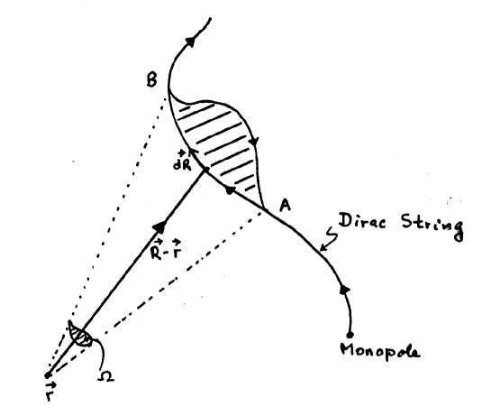
Figure 2.3: The effect on the vector potential of deforming a Dirac string.

The second term vanishes at any point $\vec{r}$ not on the surface and can be dropped. The first term is the gradient of the solid angle $\Omega$, subtended by the surface $S$, when viewed from the point $\vec{r}$:

$$\delta\vec{A}\left(\vec{r}\right)=\frac{g}{4\pi}\vec{\nabla}\left(\int_{S}d\vec{s}\cdot\vec{\nabla}_{R}\frac{1}{\left|\vec{r}-\vec{R}\right|}\right)=-\frac{g}{4\pi}\vec{\nabla}\int_{S}\;d\vec{s}\cdot\left(\vec{r}-\vec{R}\right)\frac{1}{\left|\vec{r}-\vec{R}\right|^{3}}=-\frac{g}{4\pi}\vec{\nabla}\Omega\left(\vec{r}\right)$$ (2.79)

To see why, consider first a very small surface $\delta\vec{s}$, such that $\left|\vec{r}-\vec{R}\right|$ remains essentially constant. Then $\delta\vec{s}\cdot\left(\vec{r}-\vec{R}\right)\frac{1}{\left|\vec{r}-\vec{R}\right|^{3}}=\frac{1}{\left|\vec{r}-\vec{R}\right|^{2}}\left(\delta\vec{s}\cdot\frac{\vec{r}-\vec{R}}{\left|\vec{r}-\vec{R}\right|}\right)=\delta\Omega_{s}$. A finite surface $S$ can be decomposed into small surfaces bounded by small contours which overlap (and therefore cancel each other) everywhere except on the boundary of the surface, that is, on the path $C$. The result (2.79) follows.

The expression (2.79) shows that $\delta\vec{A}$ is a gradient. The deformation of the string therefore adds a gradient to the vector potential $\vec{A}$ and this corresponds to a gauge transformation. A deformation of the Dirac string can therefore be compensated by a gauge transformation.

This is, however, only true at points which do not lie on the surface $S$. Indeed, the solid angle $\Omega\left(\vec{r}\right)$ is a discontinuous function of $\vec{r}$. The vector $\vec{r}-\vec{R}$ changes sign as the point $\vec{r}$ crosses the surface. If the point $\vec{r}$ lies close to and on one side of the surface $S$ (the shaded area in Fig. 2.3), the solid angle $\Omega\left(\vec{r}\right)$ is equal to $2\pi$ (half a sphere). As soon as point $\vec{r}$ crosses the surface, the solid angle switches to $-2\pi$. Thus the solid angle $\Omega\left(\vec{r}\right)$ undergoes a discontinuous variation of $4\pi$ as the point crosses the surface $S$. As a result, the gauge transformation which compensates a deformation of the Dirac string is a singular gauge transformation. This point will be further discussed in Sect. 3.3.2.

Consider the wavefunction $\psi\left(\vec{r}\right)$ of an electron. (We consider an electron because it is a particle with the smallest observed electric charge.) When the vector potential undergoes a gauge transformation $\vec{A}\rightarrow\vec{A}-\frac{g}{4\pi}\vec{\nabla}\Omega$, the electron wavefunction undergoes the gauge transformation $\psi\rightarrow e^{ie\frac{g\Omega}{4\pi}}\psi$. This means that, on either side of the surface $S$, the electron wavefunction differs by a phase $e^{ie\frac{g\Omega}{4\pi}}=e^{ieg}$. This would make the Dirac string observable, unless we impose the condition:

$$eg=2n\pi$$ (2.80)

where $n$ is an integer. The expression (2.80) is the charge quantization condition proposed by Dirac. In his own words, ”the mere existence of one [magnetic] pole of strength $g$ would require all electric charges to be quantized in units of $2\pi n/g$ and similarly, the existence of one [electric] charge would require all [magnetic] poles to quantized. The quantization of electricity is one of the most fundamental and striking features of atomic physics, and there seems to be no explanation of it apart from the theory of poles. This provides some grounds for believing in the existence of these poles” [9]. This was written in 1948. Dirac used a different argument to prove the quantization rule (2.80). The proof given above is taken from Chap. 6 of Jackson’s Classical Electrodynamics [47]. There have been many other derivations [48, 49]. For a late 2002 reflection of Jackiw on the subject, see reference [50].

The discontinuity of the solid angle $\Omega\left(\vec{r}\right)$ implies that, on the surface $S$, we have $\vec{\nabla}\times\left(\vec{\nabla}\Omega\right)\neq 0$, so that, for example, $\left(\partial_{x}\partial_{y}-\partial_{y}\partial_{x}\right)\Omega\neq 0$. To see this, consider the line integral $\oint_{L}\left(\vec{\nabla}\Omega\right)\cdot d\vec{l}$ taken along a path $L$ which crosses the surface $S$ (the shaded area on Fig. 2.3). The integral is, of course, equal to the discontinuity of $\Omega$ across the surface $S$. It is therefore equal to $4\pi$. However, in view of Stoke’s theorem (A.93, we have:

$$\oint_{L}\left(\vec{\nabla}\Omega\right)\cdot d\vec{l}=\int_{S\left(L\right)}d\vec{s}\cdot\left(\vec{\nabla}\times\left(\vec{\nabla}\Omega\right)\right)=4\pi$$ (2.81)

where $S\left(L\right)$ is the surface bounded by the path $L$. It follows that $\vec{\nabla}\times\left(\vec{\nabla}\Omega\right)\neq 0$ on the surface $S$.

2.10 The way Dirac originally argued for the string

In his 1948 paper [9], Dirac had an elegant way of conceiving the string term in order to accommodate magnetic monopoles. He first noted that the relation $F_{\mu\nu}=\partial_{\mu}A_{\nu}-\partial_{\nu}A_{\mu}$ implied the absence of magnetic charges. In an attempt to preserve this relation as far as possible, he argued as follows. If the field tensor had the form $F_{\mu\nu}=\partial_{\mu}A_{\nu}-\partial_{\nu}A_{\mu}$, then the magnetic field would be $\vec{H}=\vec{\nabla}\times\vec{A}$. The flux of the magnetic field through any closed surface $S$ would then vanish because of the divergence theorem (A.90):

$$\int_{S}\vec{H}.d\vec{s}=\int_{S}\left(\vec{\nabla}\times\vec{A}\right).d\vec{s}=\int_{V}d^{3}r\;\vec{\nabla}.\left(\vec{\nabla}\times\vec{A}\right)=0$$ (2.82)

where $V$ is the volume enclosed by the surface $S$ and $d\vec{s}$ a surface element directed outward normal to the surface. However, if the surface $S$ encloses a magnetic monopole of charge $g$, then the Maxwell equation $\vec{\nabla}.\vec{H}=g\delta\left(\vec{r}\right)$ states that the total magnetic flux crossing the surface $S$ should equal the magnetic charge $g$ of the monopole:

$$\int_{S}\vec{H}.d\vec{s}=\int_{V}d^{3}r\;\vec{\nabla}.\vec{H}=\int_{V}d^{3}r\;g\delta\left(\vec{r}\right)=g$$ (2.83)

Dirac concluded that ”the equation $F_{\mu\nu}=\partial_{\mu}A_{\nu}-\partial_{\nu}A_{\mu}$ must then fail somewhere on the surface $S$” and he assumed that it fails at only one point on the surface $S$. ”The equation will then fail at one point on every closed surface surrounding the magnetic monopole, so that it will fail on a line of points”, which he called a string. ”The string may be any curved line, extending from the pole to infinity or ending at another monopole of equal and opposite strength. Every magnetic monopole must be at the end of such a string.” Dirac went on to show that the strings are unphysical variables which do not influence physical phenomena and that they must not pass through electric charges. He therefore replaced the expression $\vec{H}=\vec{\nabla}\times\vec{A}$, by the modified expression:

$$\vec{H}=\vec{\nabla}\times\vec{A}+\vec{H}_{st}$$ (2.84)

• Exercise: Try the formulate the theory in terms of two strings, each one carrying a fraction of the flux of the magnetic field. Under what conditions can a monopole be attached to two strings?

2.11 Electromagnetism expressed in terms of the gauge field $B^{\mu}$ associated to the dual field tensor $\bar{F}^{\mu\nu}$

The scheme developed in Sect. 2.2 is useful when a model action is expressed in terms of the vector potential $A^{\mu}$ related to the field tensor $F=\partial\wedge A-\bar{G}$ and when magnetic charges and currents are present. We shall however be interested in the Landau-Ginzburg model of a dual superconductor, which is expressed in terms of the potential $B^{\mu}$ associated to the dual tensor $\bar{F}^{\mu\nu}$ and in which (color) electric charges are present. We cannot write the dual field tensor in the form $\bar{F}=\partial\wedge B$ because that would imply that $\partial\cdot F=-\partial\cdot\overline{\partial\wedge B}=0$, which would preclude the existence of electric charges. The way out, of course, is to modify the expression of $\bar{F}^{\mu\nu}$ by adding a string term $\bar{G}^{\mu\nu}$ and writing the dual field tensor in the form:

$$\bar{F}=\partial\wedge B+\bar{G}\;\;\;\;\;\;F=-\overline{\partial\wedge B}+G$$ (2.85)

We require the string term $G$ to be independent of $B$ and to satisfy the equation:

$$\partial\cdot G=j$$ (2.86)

Note that, in the expression (2.85), the string term $G$ is added to the field tensor $F$, whereas, in the Dirac formulation (2.10), the string term is added to the field tensor $\bar{F}$. The roles of $F$ and $\bar{F}$ are indeed interchanged when we express electromagnetism in terms of the gauge field $B^{\mu}$.

This way, the first Maxwell equation $\partial\cdot F=\partial\cdot G=j$ is satisfied independently of the field $B^{\mu}$. The latter is determined by the second Maxwell equation $\partial\cdot\bar{F}=j_{mag}$, namely:

$$\partial\cdot\left(\partial\wedge B\right)+\partial\cdot\bar{G}=j_{mag}$$ (2.87)

where $j_{mag}^{\mu}$ is a magnetic current, which in the dual Landau-Ginzburg model, is provided by a gauged complex scalar field. The equation for $B^{\mu}$ may be obtained from the variation of the action:

$$I_{j,j_{mag}}\left(B\right)=\int d^{4}x\left(-\frac{1}{2}\bar{F}^{2}-j_{mag}\cdot B\right)=\int d^{4}x\left(-\frac{1}{2}\left(\partial\wedge B+\bar{G}\right)^{2}-j_{mag}\cdot B\right)$$ (2.88)

with respect to the gauge field $B^{\mu}$. The action (2.88) is invariant under the gauge transformation $B\rightarrow B+\left(\partial\beta\right)$ provided that $\partial\cdot j_{mag}=0$.

The source term $G$ has to satisfy two conditions. The first is the equation $\partial\cdot G=j$. The second is: $\partial\cdot\bar{G}\neq 0$. Otherwise, the electric current decouples from the system. String solutions satisfy the second condition, whereas a form, such as $G=\partial\wedge A$ does not.

We define:

$$B^{\mu}=\left(\vec{B},\chi\right)\;\;\;\;\;\;\partial^{\mu}=\frac{\partial}{\partial x_{\mu}}=\left(\partial_{t},-\vec{\nabla}\right)\;\;\;\;\;\;j^{\mu}=\left(\rho,\vec{j}\right)$$ (2.89)

We can express the string term $G^{\mu\nu}$ and its dual $\overline{G}^{\mu\nu}$ in terms of two euclidean 3-vectors $\vec{E}_{st}$ and $\vec{H}_{st}$ in the same way as the field tensor $F^{\mu\nu}$ is expressed in terms of the electric and magnetic fields. In analogy with (2.3) we define:

$$E_{st}^{i}=-G^{0i}=\frac{1}{2}\varepsilon^{0ijk}\bar{G}_{jk}\;\;\;\;\;\;H_{st}^{i}=-\bar{G}^{0i}=-\frac{1}{2}\varepsilon^{0ijk}G_{jk}$$ (2.90)

Be careful not to confuse these definitions with the definitions (2.14)!

With a field tensor of the form (2.85), the electric and magnetic fields can be obtained from (2.3) with the result:

$$\vec{E}=-\vec{\nabla}\times\vec{B}+\vec{E}_{st}\;\;\;\;\;\;\vec{H}=-\partial_{t}\vec{B}-\vec{\nabla}\chi+\vec{H}_{st}$$ (2.91)

The equation $\partial\cdot G=j$ translates to:

$$\vec{\nabla}\cdot\vec{E}_{st}=\rho\;\;\;\;\;\;-\partial_{t}\vec{E}_{st}+\vec{\nabla}\times\vec{H}_{st}=\vec{j}$$ (2.92)

and we have:

$$-\frac{1}{2}\bar{F}^{2}=-\frac{1}{2}\left(\partial\wedge B+\bar{G}\right)^{2}=\frac{1}{2}\left(-\partial_{t}\vec{B}-\vec{\nabla}\chi+\vec{H}_{st}\right)^{2}-\frac{1}{2}\left(-\vec{\nabla}\times\vec{B}+\vec{E}_{st}\right)^{2}$$ (2.93)

The source term $\vec{E}^{st}$ has to satisfy two conditions. The first is the equation $\vec{\nabla}\cdot\vec{E}_{st}=\rho$. The second is that $\vec{\nabla}\times\vec{E}^{st}\neq 0$.

The magnetic charge density and current are given by (2.8):

$$\rho_{mag}=\vec{\nabla}\cdot\vec{H}=\vec{\nabla}\cdot\left(-\partial_{t}\vec{B}-\vec{\nabla}\chi+\vec{H}_{st}\right)$$

$$\vec{j}_{mag}=-\partial_{t}\vec{H}-\vec{\nabla}\times\vec{E}=-\partial_{t}\left(-\partial_{t}\vec{B}-\vec{\nabla}\chi+\vec{H}_{st}\right)-\vec{\nabla}\times\left(-\vec{\nabla}\times\vec{B}+\vec{E}_{st}\right)$$ (2.94)

Consider the case where the system consists of a static point electric charge $e$ at the position $\vec{R}_{1}$ and a static electric charge $-e$ at the position $\vec{R}_{2}$. The charge density is then:

$$\rho\left(\vec{r}\right)=e\delta\left(\vec{r}-\vec{R}_{1}\right)-e\delta\left(\vec{r}-\vec{R}_{2}\right)$$ (2.95)

and the electric current $\vec{j}$ vanishes. In that case, we can use a string term of the form:

$$\vec{E}_{st}\left(\vec{r}\right)=e\int_{L}d\vec{R}\,\,\delta\left(\vec{r}-\vec{R}\right)\;\;\;\;\;\;\;\;\;\vec{H}_{st}\left(\vec{r}\right)=0$$ (2.96)

where the line integral follows a path $L$ (which is the string), which stems from the charge $e$ at the point $\vec{R}_{1}$ and terminates at the charge $-e$ at the point $\vec{R}_{2}$. A point on the path $L$ can be parametrized by a function $\vec{R}\left(s\right)$ such that:

$$\vec{R}_{1}=\vec{R}\left(s_{1}\right)\;\;\;\;\;\;\;\vec{R}_{2}=\vec{R}\left(s_{2}\right)\;\;\;\;\;\;\;\;d\vec{R}=ds\,\frac{d\vec{R}}{ds}$$ (2.97)

in which case the line integral (2.96) acquires the more explicit form:

$$\vec{E}_{st}\left(\vec{r}\right)=e\int_{s_{1}}^{s_{2}}ds\frac{d\vec{R}}{ds}\,\,\delta\left(\vec{r}-\vec{R}\left(s\right)\right)$$ (2.98)

The argument which follows equation (2.43) can be repeated here with the result:

$$\vec{\nabla}_{r}\cdot\vec{E}_{st}=e\int_{L}d\vec{R}\cdot\vec{\nabla}_{r}\,\,\delta\left(\vec{r}-\vec{R}\right)=-e\int_{L}d\vec{R}\cdot\vec{\nabla}_{R}\,\,\delta\left(\vec{r}-\vec{R}\right)=e\delta\left(\vec{r}-\vec{R}_{1}\right)-e\delta\left(\vec{r}-\vec{R}_{2}\right)$$ (2.99)

If we had a single electric charge $e$ at the point $\vec{R}_{1}$ the string would extend out to infinity.

Many calculations are performed with straight line strings, discussed in Sect. 2.6, and which is the following solution of the equation $\partial\cdot G=j$:

$$G=\frac{1}{n\cdot\partial}n\wedge j\;\;\;\;\;\;\;\;\;G^{\mu\nu}=\frac{1}{n\cdot\partial}\left(n^{\mu}j^{\nu}-n^{\nu}j^{\mu}\right)$$ (2.100)

where $n^{\mu}$ is a given fixed vector and $n\cdot\partial=n_{\mu}\partial^{\mu}$. This form solves the equation $\partial\cdot G=j$ if $\partial_{\mu}j^{\mu}=0$, that is, if the electric current is conserved. If we choose $n^{\mu}$ to be space-like, the string terms $\vec{E}_{st}$ and $\vec{H}_{st}$ are given by:

$$n^{\mu}=\left(0,\vec{n}\right),\;\;\;\;\;\;n\cdot\partial=\vec{n}\cdot\vec{\nabla},\;\;\;\;\;\;\vec{E}_{st}=\frac{\vec{n}}{\vec{n}\cdot\vec{\nabla}}\rho,\;\;\;\;\;\;\vec{H}_{st}=-\frac{1}{\vec{n}\cdot\vec{\nabla}}\vec{n}\times\vec{j}$$ (2.101)

Consider the Fourier transform of the source term $\vec{E}_{st}$:

$$\vec{E}_{st}\left(\vec{k}\right)=\int d^{3}r\;e^{i\vec{k}\cdot\vec{r}}\frac{\vec{n}}{\vec{n}\cdot\vec{\nabla}}\rho\left(\vec{r}\right)=-\frac{\vec{n}}{i\vec{n}\cdot\vec{k}}\;\rho\left(\vec{k}\right)$$ (2.102)

The inverse Fourier transform is:

$$\vec{E}_{st}\left(\vec{r}\right)=-\frac{1}{\left(2\pi\right)^{3}}\int d^{3}k\;e^{-i\vec{k}\cdot\vec{r}}\frac{\vec{n}}{i\vec{n}\cdot\vec{k}}\;\int d^{3}r^{\prime}e^{-i\vec{k}\cdot\vec{r}^{\prime}}\rho\left(\vec{r}^{\prime}\right)$$ (2.103)

Let us choose the $z$-axis to be parallel to $\vec{n}$, so that $\frac{\vec{n}\cdot\vec{k}}{n}=k_{z}$ and $\frac{\vec{n}}{n}=\vec{e}_{\left(z\right)}$ where $\vec{e}_{\left(z\right)}$ is the unit vector pointing in the $z$-direction. We obtain:

$$\vec{E}_{st}\left(\vec{r}\right)=-\vec{e}_{\left(z\right)}\frac{1}{\left(2\pi\right)^{3}}\int d^{3}k\;e^{-i\vec{k}\cdot\vec{r}}\frac{1}{ik_{z}}\;\int d^{3}r^{\prime}e^{-i\vec{k}\cdot\vec{r}^{\prime}}\rho\left(\vec{r}^{\prime}\right)$$ (2.104)

We obtain:

$$\vec{E}_{st}\left(\vec{r}\right)=\vec{e}_{\left(z\right)}\int d^{3}r^{\prime}\delta\left(x-x^{\prime}\right)\delta\left(y-y^{\prime}\right)\theta\left(z-z^{\prime}\right)\rho\left(\vec{r}^{\prime}\right)=\vec{e}_{\left(z\right)}\int_{0}^{\infty}dz^{\prime}\;\rho\left(x,y,z-z^{\prime}\right)$$ (2.105)

Let

$$\vec{R}\left(z^{\prime}\right)=\left(0,0,z^{\prime}\right)\;\;\;\;\;\;d\vec{R}=\vec{e}_{\left(z\right)}dz^{\prime}\;\;\;\;\;\;\vec{r}-\vec{R}=\left(x,y,z-z^{\prime}\right)$$ (2.106)

We obtain:

$$\vec{E}_{st}\left(\vec{r}\right)=\int_{0}^{\infty}dz^{\prime}\frac{dR\left(z^{\prime}\right)}{dz^{\prime}}\;\rho\left(\vec{r}-\vec{R}\left(z^{\prime}\right)\right)=\int_{L}d\vec{R}\;\rho\left(\vec{r}-\vec{R}\right)$$ (2.107)

where the path $L$ is a straight line, starting at the origin and running parallel to the $z$-axis. The expression (2.107) provides for a determination of the operator $\frac{\vec{n}}{\vec{n}\cdot\vec{\nabla}}$ used in (2.101). For example, if the system has a single charge $e$ at the point $\vec{R}_{1}$, the density is $\rho\left(\vec{r}\right)=e\delta\left(\vec{r}-\vec{R}_{1}\right)$ and the expression yields a string term $\vec{E}_{st}\left(\vec{r}\right)$ which stems from the point $\vec{R}_{1}$ and extends to infinity parallel to the $z$-axis. If there is an additional charge $-e$ located at the point $\vec{R}_{2}$, then the expression will yield an additional parallel string, stemming from the charge $-e$ and extending to infinity parallel to the $z$-axis. It will not be a string joining the two charges, unless the two charges happen to be located along the $z$-axis. Of course, if the strings can be deformed so as to merge at some point, then the two strings become equivalent to a single string joining the equal and opposite charges.

Chapter 3 The Landau-Ginzburg model of a dual superconductor

We shall describe color confinement in the QCD ground state in terms of a dual superconductor, which differs from usual metallic superconductors in that the roles of the electric and magnetic fields are exchanged. The dual superconductor will be described in terms of a suitably adapted Landau-Ginzburg model of superconductivity. The original model was developed in 1950 by Ginzburg and Landau [8]. Particle physicists refer to it today as the Dual Abelian Higgs model. The crucial property of the dual superconductor will be the Meissner effect [51], which expels the electric field (instead of the magnetic field, as in a usual superconductors). As a result, the color-electric field which is produced, for example, by a quark-antiquark pair embedded in the dual superconductor, acquires the shape of a color flux tube, thereby generating an asymptotically linear confining potential.

It is easy to formulate a model in which the Meissner effect applies to the electric field. All we need to do is to formulate the Landau-Ginzburg theory in terms of a vector potential $B^{\mu}$ associated to the dual field tensor $\bar{F}^{\mu\nu}$, as in Sect.2.11. For an early review and a historical background, see the 1975 paper of Jevicki and Senjanovic [6]. The presentation given below owes a lot to the illuminating account of superconductivity given in Sect.21.6 of vol.2 of Steven Weinberg’s Quantum Theory of Fields [52]. We first study the dual Landau-Ginzburg model with no reference to the color degrees of freedom. The way the latter are incorporated is discussed in Chap.5.

3.1 The Landau-Ginzburg action of a dual superconductor

The Landau-Ginzburg (Abelian Higgs) model is expressed in terms of a gauged complex scalar field $\psi$, which, presumably, represents a magnetic charge condensate. The model action is:

$$I_{j}\left(B,\psi,\psi^{\ast}\right)=\int d^{4}x\left(-\frac{1}{4}\overline{F}_{\mu\nu}\overline{F}^{\mu\nu}+\frac{1}{2}\left(D_{\mu}\psi\right)\left(D_{\mu}\psi\right)^{\ast}-\frac{1}{2}b\left(\psi\psi^{\ast}-v^{2}\right)^{2}\right)$$ (3.1)

where $\psi$ is the complex scalar field and $\bar{F}^{\mu\nu}$ the dual field tensor. The covariant derivative is $D_{\mu}=\partial_{\mu}+igB_{\mu}$, where $B^{\mu}$ is a vector potential, and:

$$\left(D_{\mu}\psi\right)=\left(\partial_{\mu}\psi+igB_{\mu}\psi\right)\;\;\;\;\;\left(D_{\mu}\psi\right)^{\ast}=\left(\partial_{\mu}\psi^{\ast}-igB_{\mu}\psi^{\ast}\right)$$ (3.2)

The dimensionless constant $g$ can be viewed as a magnetic charge. As explained in Sect.2.11, the presence of electric charges and currents can be taken into account by adding a string term $\bar{G}$ to the dual field strength tensor, which is:

$$\bar{F}^{\mu\nu}=\left(\partial\wedge B\right)^{\mu\nu}+\bar{G}^{\mu\nu}\;\;\;\;\;\;F^{\mu\nu}=-\left(\overline{\partial\wedge B}\right)^{\mu\nu}+G^{\mu\nu}$$ (3.3)

The string term is related to the electric current by the equation:

$$\partial_{\alpha}G^{\alpha\mu}=j^{\mu}$$ (3.4)

The Landau-Ginzburg action (3.1) is invariant under the abelian gauge transformation:

$$\Omega\left(x\right)=e^{-ig\beta\left(x\right)}\;\;\;\;\;\;\;D_{\mu}\rightarrow\Omega D_{\mu}\Omega^{\dagger}$$

$$B_{\mu}\rightarrow B_{\mu}+\left(\partial_{\mu}\beta\right)\;\;\;\;\;\;\psi\rightarrow e^{-ig\beta}\psi$$ (3.5)

The last term of the action is a potential which drives the scalar field to a non-vanishing expectation value $\psi\psi^{*}=v^{2}$ in the ground state of the system. The superconducting phase occurs when $\psi\psi^{*}=v^{2}\neq 0$, and it will model the color-confined phase of QCD. The normal phase occurs when $\psi\psi^{*}=0$ and it represents the perturbative phase of QCD. The model parameter $v$ may be temperature and density dependent, and its variation can drive the system to the normal phase. Of course, other processes may also contribute to the phase transition. Note that, when $\psi\psi^{*}\neq 0$, the action (3.8) is not invariant under the gauge transformation $B\rightarrow B+\left(\partial\beta\right)$ of the field $B^{\mu}$ alone because, loosely speaking, the gauge field $B^{\mu}$ acquires a squared mass $g^{2}\psi\psi^{*}$. In the compact notation described in App.A, the action reads:

$$I_{j}\left(B,\psi,\psi^{*}\right)=\int d^{4}x\left(-\frac{1}{2}\left(\partial\wedge B+\bar{G}\right)^{2}+\frac{1}{2}\left|\partial\psi+igB\psi\right|^{2}-\frac{1}{2}b\left(\psi\psi^{*}-v^{2}\right)^{2}\right)$$ (3.6)

The physical content of the model is often more transparent in a polar representation of the complex field $\psi$:

$$\psi\left(x\right)=S\left(x\right)e^{ig\varphi\left(x\right)}\;\;\;\;\;\;\psi^{*}\left(x\right)=S\left(x\right)e^{-ig\varphi\left(x\right)}$$ (3.7)

The Landau-Ginzburg action (3.1) can be expressed in terms of the real fields $S$ and $\varphi$:

$$I_{j}\left(B,\varphi,S\right)=\int d^{4}x\left(-\frac{1}{2}\left(\partial\wedge B+\bar{G}\right)^{2}+\frac{g^{2}S^{2}}{2}\left(B+\partial\varphi\right)^{2}+\frac{1}{2}\left(\partial S\right)^{2}-\frac{1}{2}b\left(S^{2}-v^{2}\right)^{2}\right)$$ (3.8)

The action (3.8) is invariant under the gauge transformation:

$$B\rightarrow B+\left(\partial\beta\right)\;\;\;\;\;\;\varphi\rightarrow\varphi-\beta\;\;\;\;\;\;S\rightarrow S$$ (3.9)

In the ground state of the system, $S=v$, and fluctuations of the scalar field $S$ describe a scalar particle with a mass:

$$m_{H}=2v\sqrt{b}$$ (3.10)

Particle physicists like to refer to $S$ as a Higgs field and to $m_{H}$ as a Higgs mass. The field $\varphi$ remains massless and is sometimes referred to as a Goldstone field. The gauge field develops a mass:

$$m_{V}=gv$$ (3.11)

Properties of superconductors are often described in terms of a penetration depth $\lambda$ and a correlation length $\xi$, which are equal to the inverse vector and Higgs masses:

$$\lambda=\frac{1}{m_{V}}\;\;\;\;\;\;\xi=\frac{1}{m_{H}}$$ (3.12)

In usual metallic superconductors, the penetration length is the distance within which an externally applied magnetic field disappears inside the superconductor. In our dual superconductor, the penetration length $\lambda$ will measure the distance within which the electric field and the magnetic current vanish outside the flux-tube which develops, for example, between a quark and an antiquark. The correlation length is related to the distance within which the scalar field acquires its vacuum value $S=v$. It is also a measure of the energy difference, per unit volume, of the normal and superconducting phase, usually referred to as the bag constant:

$$\mathcal{B}=\frac{1}{8}m_{H}^{2}v^{2}=\frac{v^{2}}{8\xi^{2}}=\frac{m_{V}^{2}}{8g^{2}\xi^{2}}$$ (3.13)

In type I superconductors (pure metals except niobium) $\xi>\lambda$ and $m_{V}>m_{H}$. In type II superconductors (alloys and niobium) $\lambda>\xi$ and $m_{H}>m_{V}$. In Sect. 3.4 we shall see that the dual superconductors which model the confinement of color charge have $m_{H}\preceq m_{V}$. They are close to the boundary which separates type I and type II superconductors. The London limit (Sect. 3.6), in which it is assumed that $b\rightarrow\infty$ so that $m_{H}\gg m_{V}$, is an extreme example of a type II superconductor. In type II superconductors, the only stable vortex lines are those with minimum flux. In type I superconductors, vortices attract each other whereas they repel each other in type II superconductors. Useful reviews of these properties can be found in Chap.21.6 (volume 2) of Weinberg’s ”Quantum Theory of Fields” [52] and in Chap.4.3 of Vilenkin and Shellard’s ”Cosmic Strings and Other Topological Defects” [53].

3.2 The Landau-Ginzburg action in terms of euclidean fields

Let us write:

$$B^{\mu}=\left(\chi,\vec{B}\right)$$ (3.14)

and let us express the antisymmetric source term $G^{\mu\nu}$ in terms of the two vectors $\vec{E}^{st}$ and $\vec{H}^{st}$ as in (2.90). The action (3.1) can then be broken down to the form:

$$I_{j}\left(\psi,\psi^{*},\vec{B},\chi\right)=\int d^{4}x$$

$$\left[\frac{1}{2}\left(-\partial_{t}\vec{B}-\vec{\nabla}\chi+\vec{H}_{st}\right)^{2}-\frac{1}{2}\left(-\vec{\nabla}\times\vec{B}+\vec{E}_{st}\right)^{2}+\frac{1}{2}\left(\partial_{t}\psi+ig\chi\psi\right)\left(\partial_{t}\psi^{*}-ig\chi\psi^{*}\right)\right.$$

$$\left.-\frac{1}{2}\left(\vec{\nabla}\psi-ig\vec{B}\psi\right)\left(\vec{\nabla}\psi^{*}+ig\vec{B}\psi^{*}\right)-\frac{1}{2}b\left(\psi\psi^{*}-v^{2}\right)^{2}\right]$$ (3.15)

Since no time derivative acts on the field $\chi$, it acts as the constraint $\frac{\delta I}{\delta\chi}=0$, namely:

$$\vec{\nabla}\cdot\left(-\partial_{t}\vec{B}-\vec{\nabla}\chi+\vec{H}_{st}\right)+\frac{ig}{2}\left(\psi\partial_{t}\psi^{*}-\psi^{*}\partial_{t}\psi\right)+g^{2}\chi\psi\psi^{*}=0$$ (3.16)

The Eq.(3.4) which relates the source terms to the electric charge density and current reads:

$$\vec{\nabla}\cdot\vec{E}_{st}=\rho\;\;\;\;\;\;-\partial_{t}\vec{E}_{st}+\vec{\nabla}\times\vec{H}_{st}=\vec{j}$$ (3.17)

3.3 The flux tube joining two equal and opposite electric charges

Consider a system composed of two static equal and opposite electric charges $\pm e$ placed on the $z$-axis at equal distances from the origin and separated by a distance $R$. The charge density is then:

$$\rho\left(\vec{r}\right)=e\delta\left(\vec{r}-\vec{R}_{1}\right)-e\delta\left(\vec{r}-\vec{R}_{2}\right)\;\;\;\;\;\;\vec{R}_{1}=\left(0,0,-\frac{R}{2}\right)\;\;\;\;\;\;\vec{R}_{2}=\left(0,0,\frac{R}{2}\right)$$ (3.18)

The electric current is then $j^{\mu}=\delta^{\mu 0}\rho$ with $\vec{j}=0$. As shown in Sect.2.11, the string terms satisfy the equations:

$$\vec{\nabla}\cdot\vec{E}^{st}=\rho\;\;\;\;\;\;\;\vec{\nabla}\times\vec{E}^{st}\neq 0\;\;\;\;\;\;\vec{H}_{st}\left(\vec{r}\right)=0$$ (3.19)

Note the condition $\vec{\nabla}\times\vec{E}^{st}\neq 0$. If this condition is not satisfied, the electric density decouples from the system, as can be seen on the expression (3.22) of the energy. String solutions are designed to avoid this.

The string term $\vec{E}^{st}$ has the form (2.96):

$$\vec{E}_{st}\left(\vec{r}\right)=e\int_{\vec{R}_{1}}^{\vec{R}_{2}}d\vec{Z}\,\,\delta\left(\vec{r}-\vec{Z}\right)$$ (3.20)

where the integral follows a path $L$ (the string), which stems from the point $\vec{R}_{1}$ and terminates at the point $\vec{R}_{2}$. Following the steps described in Sect. 2.5, we can easily check that the form (3.20) satisfies the equation $\vec{\nabla}\cdot\vec{E}_{st}=\rho$ with $\rho$ given by (3.18).

When the fields are time-independent, the energy density is equal to minus the action density given by (3.15). The energy of the system is thus:

$$\mathcal{E}_{\rho}\left(\psi,\psi^{*},\vec{B},\chi\right)=\int d^{3}r\left[-\frac{1}{2}\left(\vec{\nabla}\chi\right)^{2}+\frac{1}{2}\left(-\vec{\nabla}\times\vec{B}+\vec{E}_{st}\right)^{2}-\frac{1}{2}g^{2}\chi^{2}\psi\psi^{*}\right.$$

$$\left.+\frac{1}{2}\left(\vec{\nabla}\psi-ig\vec{B}\psi\right)\left(\vec{\nabla}\psi^{*}+ig\vec{B}\psi^{*}\right)+\frac{1}{2}b\left(\psi\psi^{*}-v^{2}\right)^{2}\right]$$ (3.21)

The constraint (3.16) is satisfied with $\chi=0$. The energy becomes the following sum of positive terms:

$$\mathcal{E}_{\rho}\left(\psi,\psi^{*},\vec{B}\right)=\int d^{3}r\left[\frac{1}{2}\left(-\vec{\nabla}\times\vec{B}+\vec{E}_{st}\right)^{2}\right.$$

$$\left.+\frac{1}{2}\left(\vec{\nabla}\psi-ig\vec{B}\psi\right)\left(\vec{\nabla}\psi^{*}+ig\vec{B}\psi^{*}\right)+\frac{1}{2}b\left(\psi\psi^{*}-v^{2}\right)^{2}\right]$$ (3.22)

This expression can also be derived from the classical energy (3.168) by making the energy stationary with respect to the conjugate momenta $\vec{H}$ and $P$, as becomes time-independent fields.

3.3.1 The Ball-Caticha expression of the string term

The string term (3.20) does not depend on the fields $B,\psi$ and $\psi^{*}$. A useful trick, introduced by Ball and Caticha [54], and used in all subsequent work, consists in expressing the string term $\vec{E}^{st}$ in terms of the electric field $\vec{E}^{0}$ and the dual vector potential $\vec{B}^{0}$, which are produced by the electric charges when they are embedded in the normal vacuum where $\psi=0$. It is a way to express the longitudinal and transverse parts of the string term $\vec{E}^{st}$ in terms of the known fields $\vec{E}^{0}$ and $\vec{B}^{0}$.

The electric field $\vec{E}^{0}$ produced by the electric charges embedded in the normal vacuum is the well known Coulomb field:

$$\vec{E}^{0}\left(\vec{r}\right)=-\frac{e}{4\pi}\vec{\nabla}\left(\frac{1}{\left|\vec{r}-\vec{R}_{1}\right|}-\frac{1}{\left|\vec{r}-\vec{R}_{2}\right|}\right)=\frac{e}{4\pi}\left(\frac{\vec{r}-\vec{R}_{1}}{\left|\vec{r}-\vec{R}_{1}\right|^{3}}-\frac{\vec{r}-\vec{R}_{2}}{\left|\vec{r}-\vec{R}_{2}\right|^{3}}\right)$$ (3.23)

This electric field $\vec{E}^{0}$ can, however, also be expressed in terms of the dual potential $\vec{B}^{0}$ and the string term $\vec{E}^{st}$, using the expression (2.91):

$$\vec{E}^{0}=-\vec{\nabla}\times\vec{B}^{0}+\vec{E}^{st}$$ (3.24)

The idea is to use this equation in order to express the string term $\vec{E}^{st}$ in terms of $\vec{E}^{0}$ and $\vec{B}^{0}$.

We can calculate the dual vector potential $\vec{B}^{0}$ as in Sect. 2.7. Since no magnetic current $\vec{j}_{mag}$ occurs in the normal vacuum, the field $\vec{B}^{0}$ is given by (2.94):

$$\vec{\nabla}\times\left(\vec{\nabla}\times\vec{B}^{0}\right)=\vec{\nabla}\times\vec{E}^{st}$$ (3.25)

The string term $\vec{E}^{st}$ is given by the line integral (3.20) so that:

$$\vec{\nabla}\times\left(\vec{\nabla}\times\vec{B}^{0}\right)=e\vec{\nabla}_{r}\times\int_{L}d\vec{Z}\,\,\delta\left(\vec{r}-\vec{Z}\right)$$ (3.26)

This is an equation for the transverse part $\vec{B}_{T}^{0}$ which is the only part we need. We have $\vec{\nabla}\times\left(\vec{\nabla}\times\vec{B}^{0}\right)=-\nabla^{2}\vec{B}_{T}^{0}$ and we can use (2.69) to write the equation above in the form:

$$-\nabla_{r}^{2}\vec{B}_{T}^{0}=-\frac{e}{4\pi}\vec{\nabla}_{r}\times\int_{L}d\vec{Z}\;\nabla_{r}^{2}\frac{1}{\left|\vec{r}-\vec{Z}\right|}$$ (3.27)

so that we can take:

$$\vec{B}^{0}\left(\vec{r}\right)=\frac{e}{4\pi}\vec{\nabla}_{r}\times\int_{L}d\vec{Z}\;\frac{1}{\left|\vec{r}-\vec{Z}\right|}$$ (3.28)

From (3.24) we see that we can write the string term in the form $\vec{E}^{st}=\vec{E}^{0}+\vec{\nabla}\times\vec{B}^{0}$. We substitute this expression into the energy (3.22), with the result:

$$\mathcal{E}_{\rho}\left(\psi,\psi^{*},\vec{B}\right)=\int d^{3}r\left[\frac{1}{2}\left(-\vec{\nabla}\times\vec{B}+\vec{E}^{0}+\vec{\nabla}\times\vec{B}^{0}\right)^{2}\right.$$

$$\left.+\frac{1}{2}\left(\vec{\nabla}\psi-ig\vec{B}\psi\right)\left(\vec{\nabla}\psi^{*}+ig\vec{B}\psi^{*}\right)+\frac{1}{2}b\left(\psi\psi^{*}-v^{2}\right)^{2}\right]$$ (3.29)

Since $\vec{E}^{0}$ is a gradient, the mixed term $\vec{E}^{0}\cdot\left(\vec{\nabla}\times\left(-\vec{B}+\vec{B}^{0}\right)\right)$ vanishes. The field $\vec{E}^{0}$ contributes a simple Coulomb term to the energy:

$$\int d^{3}r\frac{1}{2}\;\vec{E}_{0}^{2}=-\frac{e^{2}}{4\pi R}\;+\;\left(terms\;independent\;of\;R\right)$$ (3.30)

In the following, we neglect the (albeit infinite) self-energy terms which are independent of $R$. The energy can thus be written in the form:

$$\mathcal{E}_{\rho}\left(\psi,\psi^{*},\vec{B}\right)=-\frac{e^{2}}{4\pi R}\;+\int d^{3}r\left[\frac{1}{2}\left(-\vec{\nabla}\times\vec{B}+\vec{\nabla}\times\vec{B}^{0}\right)^{2}\right.$$

$$\left.+\frac{1}{2}\left(\vec{\nabla}\psi-ig\vec{B}\psi\right)\left(\vec{\nabla}\psi^{*}+ig\vec{B}\psi^{*}\right)+\frac{1}{2}b\left(\psi\psi^{*}-v^{2}\right)^{2}\right]$$ (3.31)

where $\vec{B}^{0}$ is given by (3.28).

3.3.2 Deformations of the string and charge quantization

Consider the effect of deforming the string, that is, the path $L$ which defines the vector $\vec{B}^{0}\left(\vec{r}\right)$ in the expression (3.28). Let us deform a segment of the path, situated between two points $A$ and $B$ on the path. The corresponding change of $\vec{B}^{0}$ is:

$$\vec{B}^{0}\left(\vec{r}\right)\rightarrow\vec{B}^{0}\left(\vec{r}\right)+\frac{e}{4\pi}\vec{\nabla}_{r}\times\int_{C}d\vec{Z}\;\frac{1}{\left|\vec{r}-\vec{Z}\right|}$$ (3.32)

where the contour $C$ follows the initial path from $A$ to $B$ and then continues back from $B$ to $A$ along the modified path, as illustrated on Fig.2.3. The expression (3.32) is the same as the expression (2.76) and we can therefore repeat the argument given in Sect.2.9 to show that the deformation of the string $L$ adds a gradient to $\vec{B}^{0}$:

$$\vec{B}^{0}\left(\vec{r}\right)\rightarrow\vec{B}^{0}\left(\vec{r}\right)+\frac{e}{4\pi}\vec{\nabla}\Omega$$ (3.33)

where $\Omega$ is the solid angle subtended by the surface $S$, bounded by the contour $C$, viewed from the point $\vec{r}$. The energy (3.31) is changed to:

$$\mathcal{E}_{\rho}\left(\psi,\psi^{\ast},\vec{B}\right)=-\frac{e^{2}}{4\pi R}\;+\int d^{3}r\left[\frac{1}{2}\left(-\vec{\nabla}\times\vec{B}+\vec{\nabla}\times\vec{B}^{0}+\frac{e}{4\pi}\vec{\nabla}\times\left(\vec{\nabla}\Omega\right)\right)^{2}\right.$$

$$\left.+\frac{1}{2}\left(\vec{\nabla}\psi-ig\vec{B}\psi\right)\left(\vec{\nabla}\psi^{\ast}+ig\vec{B}\psi^{\ast}\right)+\frac{1}{2}b\left(\psi\psi^{\ast}-v^{2}\right)^{2}\right]$$ (3.34)

We have purposely not set to zero the term $\vec{\nabla}\times\left(\vec{\nabla}\Omega\right)$ because, as shown in Sect.2.9, the solid angle $\Omega\left(\vec{r}\right)$ is a discontinuous function of $\vec{r}.$ It undergoes a sudden change of $4\pi$ as $\vec{r}$ crosses the surface $S$ bordered by the path $C$ (the shaded area in Fig. 2.3). The Eq. (2.81) shows that $\vec{\nabla}\times\left(\vec{\nabla}\Omega\right)$ is non-vanishing on the surface $S$. We can, however, compensate for the extra term $\frac{e}{4\pi}\vec{\nabla}\times\left(\vec{\nabla}\Omega\right)$ in the energy (3.34) by performing the following singular gauge transformation:

$$\vec{B}\rightarrow\vec{B}+\frac{e}{4\pi}\left(\vec{\nabla}\Omega\right)\;\;\;\;\;\;\psi\rightarrow e^{ige\frac{\Omega}{4\pi}}\psi$$ (3.35)

which reduces the energy (3.34) to its original form (3.31). The energy (3.31) becomes thus independent of the shape of the string. The gauge transformation (3.35) is not well defined because the transformed field $e^{-ige\frac{\Omega}{4\pi}}\psi$ is a discontinuous function of $\vec{r}$ thereby making the gradient $\vec{\nabla}e^{-ige\frac{\Omega}{4\pi}}\psi$ ill defined. However, we can impose the condition:

$$eg=2n\pi$$ (3.36)

which makes the field $e^{-ige\frac{\Omega}{4\pi}}\psi$ a continuous and differentiable function of $\vec{r}$. We recover the Dirac quantization condition (2.80). Thus, deformations of the string can be compensated by singular gauge transformations.

3.3.3 The relation between the Dirac string
and the flux tube in the unitary gauge

It is convenient to express the energy (3.31) in terms of the polar representation (3.7) of the complex scalar field:

$$\mathcal{E}_{\rho}\left(\vec{B},\varphi,S\right)=-\frac{e^{2}}{4\pi R}\;+\int d^{3}r\left[\frac{1}{2}\left(-\vec{\nabla}\times\vec{B}+\vec{\nabla}\times\vec{B}^{0}\right)^{2}\right.$$

$$\left.+\frac{g^{2}S^{2}}{2}\left(\vec{B}-\vec{\nabla}\varphi\right)^{2}+\frac{1}{2}\left(\vec{\nabla}S\right)^{2}+\frac{1}{2}b\left(S^{2}-v^{2}\right)^{2}\right]$$ (3.37)

As shown in Sect.3.3.2, a modification of the shape of the string, which defines $\vec{B}_{0}$ in Eq.(3.28), adds the gradient $\frac{e}{4\pi}\vec{\nabla}\Omega$ to $\vec{B}_{0}$. The corresponding modification of the energy can be compensated by the gauge transformation

$$\vec{B}\rightarrow\vec{B}+\frac{e}{4\pi}\left(\vec{\nabla}\Omega\right)\;\;\;\;\;\;\varphi\rightarrow\varphi+ige\frac{\Omega}{4\pi}$$ (3.38)

Because the energy (3.37) is invariant under the gauge transformation:

$$\vec{B}\rightarrow\vec{B}-\vec{\nabla}\beta\;\;\;\;\;\;\varphi\rightarrow\varphi-\beta$$ (3.39)

we can choose the gauge $\beta=\varphi$, which is usually referred to as the unitary gauge. In this gauge, the field $\varphi$ vanishes and the energy (3.37) is equal to:

$$\mathcal{E}_{\rho}\left(\vec{B},S\right)=-\frac{e^{2}}{4\pi R}\;+\int d^{3}r\left[\frac{1}{2}\left(-\vec{\nabla}\times\vec{B}+\vec{\nabla}\times\vec{B}^{0}\right)^{2}\right.$$

$$\left.+\frac{g^{2}S^{2}}{2}\vec{B}^{2}+\frac{1}{2}\left(\vec{\nabla}S\right)^{2}+\frac{1}{2}b\left(S^{2}-v^{2}\right)^{2}\right]$$ (3.40)

The energy (3.40), expressed in the unitary gauge, is not independent of the shape of the string which defines the field $\vec{B}^{0}$, nor should it be, because modifications of the shape of the string are compensated by modifications of the phase $\varphi$. When, for example, flux tubes joining electric charges are calculated by minimizing the energy (3.40) expressed in the unitary gauge, the flux tubes follow and develop around the Dirac strings. For example, in Sect.3.3.5, we shall see that the string term represents the longitudinal part of the electric field. In the unitary gauge, the shapes of the Dirac strings can be chosen so as to minimize the energy. They can subsequently be deformed, by re-introducing the field $\varphi$, as in the expression (3.37) for example.

3.3.4 The flux tube calculated in the unitary gauge

When the system consists of two static equal and opposite charges, the charge density is given by (3.18) and the Dirac string is a straight line joining the two charges. The field $\vec{B}^{0}\left(\vec{r}\right)$ is given by the expression (3.28) with $d\vec{Z}=\vec{e}_{\left(z\right)}dz$, where $\vec{e}_{\left(z\right)}$ is a unit vector parallel to the $z$-axis. The explicit expression can be written in cylindrical coordinates (App.A.6.2):

$$\vec{B}^{0}\left(\vec{r}\right)=\frac{e}{4\pi}\vec{\nabla}_{r}\times\vec{e}_{\left(z\right)}\int_{-\frac{R}{2}}^{\frac{R}{2}}dz^{\prime}\;\frac{1}{\sqrt{\rho^{2}+\left(z-z^{\prime}\right)^{2}}}$$ (3.41)

Use (A.106) to get:

$$\vec{B}^{0}\left(\vec{r}\right)=\frac{e}{4\pi}\vec{e}_{\left(\theta\right)}\int_{-\frac{R}{2}}^{\frac{R}{2}}dz^{\prime}\frac{\rho}{\left(\rho^{2}+\left(z-z^{\prime}\right)^{2}\right)^{\frac{3}{2}}}$$

$$=-\vec{e}_{\left(\theta\right)}\frac{e}{4\pi}\frac{1}{\rho}\left(\frac{z-\frac{R}{2}}{\sqrt{\left(\rho^{2}+\left(z-\frac{R}{2}\right)^{2}\right)}}-\frac{z+\frac{R}{2}}{\sqrt{\left(\rho^{2}+\left(z+\frac{R}{2}\right)^{2}\right)}}\right)\equiv\vec{e}_{\left(\theta\right)}B^{0}\left(\rho,z\right)$$ (3.42)

This is an analytic expression for the field $\vec{B}^{0}$ in cylindrical coordinates. From (A.105) we can check directly that $\vec{\nabla}.\vec{B}^{0}=0$ so that $\vec{B}^{0}$ is transverse. Near the $z$-axis, where $\rho$ is small, the field $B^{0}\left(\rho,z\right)$ becomes singular:

$$B^{0}\left(\rho,z\right)\mathrel{\mathop{\rightarrow}\limits_{\rho\rightarrow 0}}=-\frac{e}{4\pi}\frac{1}{\rho}\left(\frac{z-\frac{1}{2}R}{\left|z-\frac{1}{2}R\right|}-\frac{z+\frac{1}{2}R}{\left|z+\frac{1}{2}R\right|}\right)$$

$$\;\begin{array}[]{l}=\frac{e}{2\pi\rho}\;\;\;when\;\;-\frac{1}{2}R<z<\frac{R}{2}\\ =0\;\;\;\;when\;\;z<-\frac{R}{2}\;\;\;and\;\;\;z>\frac{R}{2}\end{array}$$ (3.43)

The fields which make the energy (3.40) stationary satisfy the equations:

$$\vec{\nabla}\times\left(\vec{\nabla}\times\vec{B}\right)-\vec{\nabla}\times\left(\vec{\nabla}\times\vec{B}^{0}\right)+g^{2}S^{2}\vec{B}=0$$

$$\left[-\vec{\nabla}^{2}+2b\left(S^{2}-v^{2}\right)+g^{2}\vec{B}^{2}\right]S=0$$ (3.44)

When $\vec{B}^{0}$ has the form (3.42), a solution exists, in cylindrical coordinates, in which the fields $S$ and $\vec{B}$ have the form:

$$S\left(\vec{r}\right)=S\left(\rho,z\right)\;\;\;\;\;\;\;\;\;\;\vec{B}\left(\vec{r}\right)=\vec{e}_{\left(\theta\right)}B\left(\rho,z\right)$$ (3.45)

The field equations (3.44) reduce to the following set of coupled equations for the functions $B\left(\rho,z\right)$ and $S\left(\rho,z\right)$:

$$-\frac{\partial^{2}\left(B-B_{0}\right)}{\partial z^{2}}-\frac{\partial}{\partial\rho}\frac{1}{\rho}\left(\frac{\partial}{\partial\rho}\rho\left(B-B_{0}\right)\right)+g^{2}S^{2}B=0$$

$$-\frac{1}{\rho}\frac{\partial}{\partial\rho}\left(\rho\frac{\partial}{\partial\rho}S\right)+2b\left(S^{2}-v^{2}\right)S+g^{2}C^{2}B=0$$ (3.46)

Using (A.106), we can express the energy (3.40) in terms of the functions $S\left(\rho,z\right)$, $B\left(\rho,z\right)$ and $B^{0}\left(\rho,z\right)$:

$$\mathcal{E}_{\rho}\left(\vec{B},S\right)=-\frac{e^{2}}{4\pi R}\;+2\pi\int_{0}^{\infty}\rho d\rho\int_{-\infty}^{\infty}dz\left[\frac{1}{2}\left(\frac{\partial\left(B-B^{0}\right)}{\partial z}\right)^{2}+\frac{1}{2\rho^{2}}\left(\frac{\partial}{\partial\rho}\rho\left(B-B^{0}\right)\right)^{2}\right.$$

$$\left.+\frac{g^{2}S^{2}}{2}B^{2}+\frac{1}{2}\left(\frac{\partial S}{\partial\rho}\right)^{2}+\frac{1}{2}\left(\frac{\partial S}{\partial z}\right)^{2}+\frac{1}{2}b\left(S^{2}-v^{2}\right)^{2}\right]$$ (3.47)

We require that, far from the sources ($\rho\rightarrow\infty,\;z\rightarrow\pm\infty$), the fields should recover their ground state values $S=v$ and $B=0$. Close to the $z$-axis, the field $B\left(\rho,z\right)\approx\frac{1}{\rho}$ thereby making the electric field finite in this region. However, such a behavior would make the contribution of the term $\frac{g^{2}S^{2}}{2}B^{2}$ diverge, unless $S\rightarrow 0$ in the vicinity of the string. This is reason why the energy (as well as the string tension), calculated in the London limit, has an ultraviolet divergence (see Sect.3.3.6).

The role of the model parameters is made more explicit, if we work with the following dimensionless fields and distances:

$$B\left(\rho,z\right)-B^{0}\left(\rho,z\right)=vl\left(x,y\right)\;\;\;\;\;\;S\left(\rho,z\right)=vs\left(x,y\right)\;\;\;\;\;\;B^{0}\left(\rho,z\right)=vb_{0}\left(x,y\right)$$

$$x=gv\rho=m_{V}\rho\;\;\;\;\;\;\;\;y=gvz=m_{V}z$$ (3.48)

where $m_{H}$ and $m_{V}$ are the Higgs and vector masses (3.10) and 3.11), respectively equal to the inverse penetration and correlation lengths (3.12). The energy acquires the form:

$$\mathcal{E}_{R}\left(l,s\right)=-\frac{e^{2}}{4\pi R}+\frac{m_{V}}{g^{2}}2\pi\int_{0}^{\infty}xdx\int_{-\infty}^{\infty}dy\left[\frac{1}{2}\left(\frac{\partial l}{\partial y}\right)^{2}+\frac{1}{2x^{2}}\left(\frac{\partial}{\partial x}xl\right)^{2}+\frac{1}{2}s^{2}\left(c-b_{0}\right)^{2}\right.$$

$$\left.+\frac{1}{2}\left(\frac{\partial s}{\partial x}\right)^{2}+\frac{1}{2}\left(\frac{\partial s}{\partial y}\right)^{2}+\frac{m_{H}^{2}}{8m_{V}^{2}}\left(s^{2}-1\right)^{2}\right]$$ (3.49)

where $\frac{m_{V}}{g^{2}}=\frac{v}{g}$.

The flux tube obtained by minimizing the energy (3.49) is calculated and displayed in the 1990 paper of Maedan, Matsubara and Suzuki [55]. The flux tube is very similar to the one obtained in lattice calculations, illustrated in Fig.3.1. A more detailed comparison to lattice data is made in Sect.3.4. More recently, progress towards analytic forms for the solutions has been reported in the 1998 paper of Baker, Brambilla, Dosch and Vairo [56].

Figure 3.1: The lines of force of the electric field between two static color-electric $SU\left(2\right)$ sources obtained from a lattice calculation in the maximal abelian projection [31].

3.3.5 The electric field and the magnetic current

The electric and magnetic fields are given by (2.91):

$$\vec{E}=-\vec{\nabla}\times\vec{B}+\vec{E}^{st}\;\;\;\;\;\;\;\vec{H}=0$$ (3.50)

The longitudinal part of the electric field is the string term $\vec{E}^{st}$ and it is given by:

$$\vec{\nabla}\cdot\vec{E}=\vec{\nabla}\cdot\vec{E}^{st}=\rho$$ (3.51)

A magnetic current (2.94) is produced by the transverse part of the electric field:

$$\vec{j}_{mag}=-\vec{\nabla}\times\vec{E}$$ (3.52)

The relation $\vec{j}_{mag}=-\vec{\nabla}\times\vec{E}$ is sometimes referred to as the ”Ampere law”.

When the fields have the cylindrical symmetry (3.45), the electric field $\vec{E}$ and the magnetic current $\vec{j}_{mag}$, given by (3.50) and (3.52), are:

$$\vec{E}\left(\rho,z\right)=-\vec{\nabla}\times\vec{B}+\vec{\nabla}\times\vec{B}^{0}+\vec{E}^{0}=\vec{e}_{\left(\rho\right)}\frac{\partial B}{\partial z}-\vec{e}_{\left(z\right)}\frac{1}{\rho}\left(\frac{\partial}{\partial\rho}\rho B\right)+\vec{E}^{0}$$

$$\vec{j}_{mag}\left(\rho,z\right)=\vec{\nabla}\times\left(\vec{\nabla}\times\vec{B}\right)-\vec{\nabla}\times\left(\vec{\nabla}\times\vec{B}_{0}\right)$$

$$=-\vec{e}_{\left(\theta\right)}\left(\frac{\partial^{2}\left(B-B^{0}\right)}{\partial z^{2}}+\frac{\partial}{\partial\rho}\frac{1}{\rho}\frac{\partial}{\partial\rho}\rho\left(B-B^{0}\right)\right)$$ (3.53)

We see that the magnetic current circulates around the $z$-axis. This is why the flux tube is often called a vortex.

3.3.6
The Abrikosov-Nielsen-Olesen vortex

When $m_{V}R\gg 1$ and $m_{H}R\gg 1$, that is, when the distance which separates the electric charges is much larger than the width of the flux tube, in regions of space where both $\rho$ and $z$ are much smaller than $R$, the source term (3.42) reduces to $\vec{B}^{0}=-\vec{e}_{\left(\theta\right)}\frac{e}{2\pi\rho}$, and this in turn implies that $\vec{\nabla}\times\vec{B}^{0}=0$. In this region of space, the fields (3.45), which are solutions of the equations (3.44), become independent of $z$ and they acquire the simpler form:

$$S\left(\vec{r}\right)=S\left(\rho\right)\;\;\;\;\;\;\;\;\;\;\vec{B}\left(\vec{r}\right)=\vec{e}_{\left(\theta\right)}B\left(\rho\right)$$ (3.54)

The electric field (3.53) points in the $z$-direction:

$$\vec{E}\left(\vec{r}\right)=-\vec{\nabla}\times\vec{B}=-\vec{e}_{\left(z\right)}\frac{1}{\rho}\frac{\partial}{\partial\rho}\left(\rho B\right)$$ (3.55)

and a magnetic current $\vec{j}_{mag}$ circulates around the $z$-axis:

$$\vec{j}_{mag}=-\vec{\nabla}\times\vec{E}=-\vec{e}_{\left(\theta\right)}\frac{\partial}{\partial\rho}\frac{1}{\rho}\frac{\partial}{\partial\rho}\rho B$$ (3.56)

A flux tube is formed which is referred to as the Abrikosov-Nielsen-Olesen vortex, studied in the 1973 paper of Nielsen and Olesen [1]. It is the analogue of the vortex lines, which were predicted to occur in superconductors by Abrikosov [57]. Being particularly simple, the Abrikosov-Nielsen-Olesen vortex has been extensively studied. In Sect. 3.4, we shall see that lattice simulations confirm the formation of an Abrikosov-Nielsen-Olesen vortex between equal and opposite charges.

The energy density becomes independent of both $z$ and $\theta$, so that, in terms of the dimensionless fields and distances (3.48), the energy per unit length along the $z$-axis reduces to:

$$\frac{\partial\mathcal{E}_{R}\left(b,s\right)}{\partial z}=2\pi v^{2}\int_{0}^{\infty}xdx\left(\frac{1}{2x^{2}}\left(\frac{\partial}{\partial x}xb\right)^{2}+\frac{1}{2}s^{2}b^{2}+\frac{1}{2}\left(\frac{\partial s}{\partial x}\right)^{2}+\frac{m_{H}^{2}}{8m_{V}^{2}}\left(s^{2}-1\right)^{2}\right)$$ (3.57)

where $b\left(x\right)=vB\left(z\right)$ and where $v^{2}=\frac{m_{V}^{2}}{g^{2}}.$ The fields $s\left(x\right)$ and $b\left(x\right)$ which make the energy stationary are the solutions of the equations:

$$-\frac{d}{dx}\frac{1}{x}\frac{d}{dx}\left(xb\right)+s^{2}b=0$$

$$-\frac{1}{x}\frac{d}{dx}x\frac{d}{dx}s+s^{2}b+\frac{m_{H}^{2}}{2m_{V}^{2}}\left(s^{2}-1\right)s=0$$ (3.58)

The boundary conditions are:

$$b\mathrel{\mathop{\rightarrow}\limits_{x\rightarrow 0}}\frac{a}{x}\;\;\;\;\;\;s\mathrel{\mathop{\rightarrow}\limits_{x\rightarrow 0}}0\;\;\;\;\;\;b\mathrel{\mathop{\rightarrow}\limits_{x\rightarrow\infty}}0\;\;\;\;\;\;s\mathrel{\mathop{\rightarrow}\limits_{x\rightarrow 0}}1$$ (3.59)

The constant $a$ can be determined from the flux of the electric field crossing a surface normal to the vortex.

The expression (3.57) is interpreted as the string tension, that is, the coefficient $\sigma$ of the asymptotically linear potential $\sigma R$ which develops between static electric charges embedded in the dual superconductor. The string tension depends on the two parameters $v$ and $\frac{m_{H}}{m_{V}}$, the ratio of the Higgs and vector masses. When $m_{H}=m_{V}$, that is, when the system is on the borderline between a type I and II superconductor, analytic solutions of the equations of motion have been found by Bogomolnyi [58]. In this Bogomolnyi limit, the string tension is given by the expression:

$$\sqrt{\sigma}=\sqrt{\frac{\pi}{g^{2}}m^{2}}\;\;\;\;\;\;m=m_{H}=m_{V}$$ (3.60)

The stability and extensions to supersymmetry have also been investigated. For a review, see the Sect.4.1 of the useful book by Vilenkin and Shellard [53]. The interaction between vortices is discussed in Sect.4.3 of that book. When $m_{H}\gg m_{V}$ (type II superconductors), vortices repel each other. When $m_{H}\ll m_{V}$ (type I superconductors) an attraction between vortices occurs.

• Exercise: Consider two equal and opposite electric charges $\pm e$ embedded in a dual superconductor. Assume that they are separated by a large distance $L$, such that a flux tube is formed, the energy of which is proportional to its length $L$. We can then write the energy of the flux tube in the form $\mathcal{E}=\alpha e^{2}L$. Study how the energy of the system varies as a function of the electric charge $e$, for a fixed value of $L$. Show that, on the average, the energy increases linearly (and not quadratically) with $e$, because several flux tubes can form.

3.3.7 Divergencies of the London limit

The London limit is the extreme case $m_{H}\gg m_{V}$ of a type II superconductor. In this limit, the energy (3.57) is be minimized when the field $s\left(x\right)$ maintains its ground state value $s=1$ ($S=v$) for all values of $x$. The equation for $b\left(x\right)$ reduces then to:

$$-\frac{d}{dx}\frac{1}{x}\frac{d}{dx}\left(xb\right)+b=0$$

which is equivalent to the following equation for the field $C\left(z\right):$

$$-\frac{d}{d\rho}\frac{1}{\rho}\frac{d}{d\rho}\left(\rho B\right)+m_{V}^{2}B=0$$ (3.61)

The solution, which vanishes far from the vortex is:

$$b\left(x\right)=aK_{1}\left(x\right)\;\;\;or\;\;\;B\left(z\right)=\frac{a}{v}K_{1}\left(m_{V}\rho\right)$$ (3.62)

However, for small values of $x$, we have:

$$x\left(K_{1}\left(x\right)\right)^{2}=\allowbreak x^{-1}+\left(-\ln\frac{1}{x}-\ln 2+\gamma-\frac{1}{2}\right)x+O\left(x^{3}\right)$$ (3.63)

so that the integral of $\frac{1}{2}s^{2}b^{2}$, in the string tension (3.57), produces a logarithmic divergence at small $x$. This is the origin of the divergence obtained in the analytic expression (3.106) of the string tension in the London limit. The electric field, far from the sources, is $\vec{E}=-\vec{\nabla}\times\vec{B}$ and it has the singular behavior $\vec{E}\left(\vec{r}\right)\simeq-\vec{e}_{\left(z\right)}\frac{a}{v}\ln\left(m_{V}\rho\right)$ when $\rho\rightarrow 0$. This singular behavior does not occur in the Landau-Ginzburg model and Fig. 3.2 shows that it is also not observed in lattice simulations.

Figure 3.2: The profiles of the electric field $E$ and of the magnetic current, marked $k_{\theta}$ on the figure, are plotted as a function of the the distance $x$ from the center of the flux tube. The results are obtained from a pure gauge $SU\left(2\right)$ lattice calculation in the maximal abelian gauge [33]. The curves are obtained from the Landau-Ginzburg model of a dual superconductor.

3.4 Comparison of the Landau-Ginzburg model with lattice data

In 1998, Bali, Schlichter and Schilling [33] compared the flux tube formed by two static sources in a $SU\left(2\right)$ lattice calculation in the maximal abelian gauge (see Chapt.4) with the Abrikosov-Nielsen-Olesen vortex formed in the Landau-Ginzburg model of a dual superconductor. They measured both the electric field and magnetic current. The flux tube is depicted in Fig.3.1. Figure 3.3 shows that the relation $\vec{j}_{mag}=-\vec{\nabla}\times\vec{E}$ between the electric field (3.55) and the magnetic current (3.56) is satisfied, and they checked that a magnetic current circulates around the flux tube. They also measured the profiles of the electric field and of the magnetic current and compared it to the corresponding expressions (3.55) and (3.56) obtained for the Abrikosov-Nielsen-Olesen vortex. Figure 3.2 shows the fit obtained with the parameters:

$$m_{V}=gv=1.23\;GeV,\;\;\;\;m_{H}=2v\sqrt{b}=1.04\;GeV$$ (3.64)

The values of $m_{V}$ and $m_{H}$ show that system is a type I superconductor, but close to the border separating type I and type II superconductors. A similar conclusion was reached by Matsubara, Ejiri and Suzuki in an earlier 1994 paper [59] for both color $SU\left(2\right)$ and $SU\left(3\right)$. The fit appears to be good enough to be significant. Note that the electric field behaves quite regularly when $x\rightarrow 0$, that is, close to the $z$-axis. This is in contradiction with the electric field calculated in the London limit. In a 1999 paper [34], Gubarev, Ilgenfritz, Polikarpov and Suzuki fitted the same lattice data with the parameters:

$$g=5.\,827\pm 0.004\;\;\;\;\;\;m_{V}=1.31\pm 0.07\;GeV\;\;\;\;\;\;m_{H}=1.36\pm 0.01\;GeV$$ (3.65)

The data are taken with a lattice spacing fitted to the observed string tension $\sqrt{\sigma_{SU\left(2\right)}}=440\;MeV$. The Landau-Ginzburg dual superconductor gives a string tension equal to:

$$\sqrt{\sigma}=400.1\pm 53.0\;MeV\approx 0.91\sqrt{\sigma_{SU\left(2\right)}}$$ (3.66)

A more recent fit reported in the 2003 paper by Koma, Ilgenfritz and Suzuki [60] yields the following parameters:

$$m_{V}=953(20)\;MeV\;\;\;\;\;\;\;m_{H}=1091(7)\;MeV$$ (3.67)

In this paper, the authors find a small dependence of the fitted coupling constant $g$ on the distance separating the quark and antiquark, which is compatible with antiscreening of the effective QCD coupling constant, derived from the Dirac quantization condition $e_{eff}=\frac{4\pi}{g}$.

Suganuma and Toki [61] argue in favor of a different set of model parameters, namely:

$$m_{V}=0.5\;GeV\;\;\;\;\;\;\;\;\;m_{H}=1.26\;MeV$$ (3.68)

which would make the QCD ground state is a type II superconductor. They do not, however, fit the profiles of the Abrikosov-Nielsen-Olesen vortex.

Figure 3.3: The figure is a lattice confirmation of the ”Ampere law” $\vec{j}_{mag}=-\vec{\nabla}\times\vec{E}$. The profiles of the magnetic current, marked $k$ on the figure and of $\vec{\nabla}\times\vec{E}$, marked $curlE$ on the figure, are plotted as a function of the distance $x$ from the center of the flux tube. The results are obtained from a pure gauge $SU\left(2\right)$ lattice calculation in the maximal abelian gauge [33].

The scalar field $S=\left|\psi\right|$, which acts as an order parameter in the Landau-Ginzburg model, does not, as such, specify the nature of the monopole condensation, assumed to occur in the QCD ground state. Similarly, the Landau-Ginzburg model of usual superconductors was not direct evidence of electron-pair condensation, which was postulated and discovered six years later [62, 63].

3.5 The dielectric function of the color-dielectric model

The Abrikosov-Nielsen-Olesen vortex may also be described in terms of the color dielectric model of T.D.Lee [64]. The model is described by the action:

$$I_{j}\left(A,\sigma\right)=\int d^{4}x\left(-\frac{1}{2}\kappa\left(\sigma\right)\left(\partial\wedge A\right)^{2}+\frac{1}{2}\left(\partial\sigma\right)^{2}-\frac{b}{2}\left(\sigma^{2}-v^{2}\right)^{2}-j\cdot A\right)$$ (3.69)

where $\kappa\left(\sigma\right)$ is a dielectric constant chosen such that is decreases regularly from $1$ to $0$ as $\sigma$ varies from zero to $v$ and where $j^{\mu}$ is a source for electric charges and currents. The equations of motion are:

$$\partial\cdot\kappa\left(\partial\wedge A\right)=j$$

$$-\partial^{2}\sigma-\frac{1}{2}\left(\partial\wedge A\right)^{2}\kappa^{\prime}\left(\sigma\right)-2b\left(\sigma^{2}-v^{2}\right)\sigma=0\;\;\;\;\;\;\left(\kappa^{\prime}\left(x\right)=\frac{\delta\kappa\left(\sigma\right)}{\delta\sigma\left(x\right)}\right)$$ (3.70)

If we define the field strength tensor to be $F^{\mu\nu}=\kappa\left(\sigma\right)\left(\partial\wedge A\right)$ then the equation of motion for $A^{\mu}$ becomes equivalent to the Maxwell equation $\partial\cdot F=j$. The system also develops a magnetic current, given by:

$$j_{mag}=\partial\cdot\bar{F}=\left(\partial\kappa\right)\cdot\overline{\partial\wedge A}$$ (3.71)

Let us write:

$$A^{\mu}=\left(\phi,\vec{A}\right)\;\;\;\;\;\;j^{\mu}=\left(\rho,\vec{j}\right)$$ (3.72)

The action can be broken down to:

$$I_{j}\left(A,\phi,\sigma\right)=\int d^{4}x\left\{\frac{1}{2}\kappa\left(-\partial_{t}\vec{A}-\vec{\nabla}\phi\right)^{2}-\frac{1}{2}\kappa\left(\vec{\nabla}\times A\right)^{2}\right.$$

$$\left.+\frac{1}{2}\left(\partial_{t}\sigma\right)^{2}-\frac{1}{2}\left(\vec{\nabla}\sigma\right)^{2}-\frac{b}{2}\left(\sigma^{2}-v^{2}\right)^{2}-\rho\phi+\vec{j}\cdot\vec{A}\right\}$$ (3.73)

The field $\phi$ imposes the constraint:

$$\vec{\nabla}\cdot\kappa\left(-\partial_{t}\vec{A}-\vec{\nabla}\phi\right)=\rho$$ (3.74)

In the presence of static charges:

$$\rho\left(x\right)=\rho\left(\vec{r}\right)\,\,\,\,\,\;\;\;\;\;\vec{j}\left(x\right)=0$$

the source $j^{\mu}$ is time independent and the fields $A^{\mu}$ and $\sigma$ may also be assumed to be time independent. The energy in the presence of static sources is:

$$\mathcal{E}_{\rho}\left(A,\phi,\sigma\right)=\int d^{3}r\left(-\frac{1}{2}\kappa\left(\vec{\nabla}\phi\right)^{2}+\frac{1}{2}\kappa\left(\vec{\nabla}\times A\right)^{2}+\frac{1}{2}\left(\vec{\nabla}\sigma\right)^{2}+\frac{b}{2}\left(\sigma^{2}-v^{2}\right)^{2}-\rho\phi\right)$$ (3.75)

and the constraint is:

$$-\kappa^{\prime}\left(\vec{\nabla}\sigma\right)\cdot\left(\vec{\nabla}\phi\right)-\kappa\nabla^{2}\phi=\rho$$ (3.76)

The energy is minimized when:

$$\vec{\nabla}\times\vec{A}=0$$ (3.77)

in which case the energy reduces to:

$$\mathcal{E}_{\rho}\left(\phi,\sigma\right)=\int d^{3}r\left(-\frac{1}{2}\kappa\left(\vec{\nabla}\phi\right)^{2}+\frac{1}{2}\left(\vec{\nabla}\sigma\right)^{2}+\frac{b}{2}\left(\sigma^{2}-v^{2}\right)^{2}-\rho\phi\right)$$ (3.78)

The field $\sigma$ which minimizes the energy satisfies the equation:

$$-\nabla^{2}\sigma+2b\left(\sigma^{2}-v^{2}\right)\sigma-\frac{1}{2}\kappa^{\prime}\left(\vec{\nabla}\phi\right)^{2}=0$$ (3.79)

Consider two static charges on the $z$-axis, placed symmetrically with respect to the origin:

$$\rho\left(\vec{r}\right)=-e\delta\left(\vec{r}-\vec{R}_{1}\right)+e\delta\left(\vec{r}-\vec{R}_{2}\right)$$ (3.80)

If the charges are far apart, then, close to the $x-y$ plane, we expect the electric field to be constant and directed along $\vec{e}_{\left(z\right)}$. A solution of equations (3.76) and (3.79) exists in cylindrical coordinates, of the form:

$$\sigma\left(\vec{r}\right)=\sigma\left(\rho\right)\;\;\;\;\;\;\phi\left(\vec{r}\right)=az$$ (3.81)

and the function $\sigma\left(\rho\right)$ is the solution of the equation:

$$-\frac{1}{\rho}\frac{d}{d\rho}\left(\rho\frac{d\sigma}{d\rho}\right)+2b\left(\sigma^{2}-v^{2}\right)\sigma-\frac{1}{2}a^{2}\kappa^{\prime}=0$$ (3.82)

In this region, the electric and magnetic fields are:

$$\vec{E}\left(\rho\right)=-\kappa\vec{\nabla}\phi=-\vec{e}_{\left(z\right)}a\kappa\left(\rho\right)\;\;\;\;\;\;\;\;\;\vec{H}=0$$ (3.83)

In this sense, lattice calculations, as well as the Landau-Ginzburg model which agrees with them, determine the function $\kappa\left[\sigma\left(\rho\right)\right]$ of the dielectric model. The magnetic current $j_{mag}^{\mu}=\left(\rho_{mag},\vec{j}_{mag}\right)$ is such that $\rho_{mag}=0$ and:

$$\;\vec{j}_{mag}=-\vec{\nabla}\times\vec{E}=\left(\vec{\nabla}\kappa\right)\times\left(\vec{\nabla}\phi\right)=\kappa^{\prime}\left(\vec{\nabla}\sigma\right)\times\left(\vec{\nabla}\phi\right)=-\vec{e}_{\left(\theta\right)}a\kappa^{\prime}\frac{d\sigma}{d\rho}$$ (3.84)

so that a magnetic current flows around the vortex which may be viewed as an Abrikosov-Nielsen-Olesen vortex.

There is however an important difference between the color-dielectric model described by the action (3.69) and the Landau-Ginzburg model. If the system, described by the color-dielectric model, is perturbed or raised to a finite temperature, the expectation value of the field $\sigma$ may be shifted to, typically, a lower value and the color dielectric function no longer vanishes, in spite of having been fine-tuned to do so in the vacuum at zero temperature. The model therefore describes the physical vacuum in terms of an unstable phase, which is not the case of the Landau-Ginzburg model which describes the superconducting phase within a finite range of temperatures.

3.6 The London limit of the Landau-Ginzburg model

The London limit of the Landau Ginzburg model is obtained by letting $b\rightarrow\infty$, which means that the Higgs mass $m_{H}$ is much larger than the vector meson mass $m_{V}.$ In that limit, the scalar field maintains its vacuum value $S=v$ and the model action (3.8) reduces to:

$$I_{j}\left(B,\varphi\right)=\int d^{4}x\left(-\frac{1}{2}\left(\partial\wedge B+\bar{G}\right)^{2}+\frac{m_{V}^{2}}{2}\left(B+\partial\varphi\right)^{2}\right)$$ (3.85)

where $m_{V}$, the mass of the vector boson, is equal to the inverse penetration depth (3.12), and where the source term $G$ is related to the electric current $j$ by the equation:

$$\partial\cdot G=j$$ (3.86)

Because of its simplicity (the action is a quadratic form of the single field $B^{\mu}$), the London limit has been extensively studied. It yields simple analytic forms for the confining potential, field strength correlators, and more. However, as explained in Sect. 3.3.4, the linear confining potential develops an ultraviolet divergence because, in the London limit, the scalar field $S$ is not allowed to vanish in the center of the flux tube. For the same reason, the electric field develops a singularity in the center of the flux tube and this is not observed in lattice simulations (see Sect. 3.4).

We shall study the London limit for a system consisting of two static electric charges. The electric current is then:

$$j^{\mu}=\left(\rho\left(\vec{r}\right),0,0,0\right)\;\;\;\;\;\;\partial^{2}j^{\mu}=-\delta_{0}^{\mu}\vec{\nabla}^{2}\rho$$

$$\rho\left(\vec{r}\right)=e\delta\left(\vec{r}-\vec{r}_{1}\right)-e\delta\left(\vec{r}-\vec{r}_{2}\right)$$ (3.87)

We work in the unitary gauge and we assume a straight line Dirac string, running from one charge to the other. In this case, we can use the form (2.100):

$$G=\frac{1}{n\cdot\partial}n\wedge j$$ (3.88)

with a space-like vector $n^{\mu}=\left(0,\vec{n}\right)$ and with $\vec{n}$ parallel to the line joining the charges:

$$\vec{n}=\vec{r}_{2}-\vec{r}_{1}$$

$$n^{\mu}=\left(0,\vec{n}\right)\;\;\;\;\;\;n^{2}=-\vec{n}^{2}\;\;\;\;\;\;n\cdot j=0\;\;\;\;\left(n\cdot\partial\right)j=\vec{n}\cdot\vec{\nabla}\rho$$ (3.89)

The equation of motion for the field $B^{\mu}$ is:

$$\partial\cdot\left(\partial\wedge B+\overline{G}\right)+m_{V}^{2}B=0$$ (3.90)

If we decompose $B^{\mu}$ into longitudinal and transverse parts using the projectors (A.10), we find that $B^{\mu}$ is transverse and equal to:

$$B=-\frac{1}{\partial^{2}+m_{V}^{2}}\partial\cdot\overline{G}$$ (3.91)

We can then eliminate the field $B^{\mu}$ from the action, which reduces to:

$$I_{j}=\int d^{4}x\left(-\frac{1}{2}\left(\partial\cdot\bar{G}\right)\frac{1}{\partial^{2}+m_{V}^{2}}\left(\partial\cdot\bar{G}\right)-\frac{1}{2}\bar{G}^{2}\right)$$ (3.92)

3.6.1 The gluon propagator

When $G$ has the form (3.88), we have:

$$\left(\partial\cdot\overline{G}\right)^{\mu}=\frac{1}{n\cdot\partial}\left(\partial\cdot\overline{n\wedge j}\right)^{\mu}=-\frac{1}{n\cdot\partial}\varepsilon^{\mu\alpha\beta\gamma}\partial_{\alpha}n_{\beta}j_{\gamma}\;\;\;\;\;\;\overline{G}^{2}=-\left(\frac{1}{n\cdot\partial}\left(n\wedge j\right)\right)^{2}$$ (3.93)

Substituting, the action (3.92) becomes:

$$I_{j}=\int d^{4}x\;\left(\frac{1}{2}j_{3}\left(\varepsilon^{\mu 123}\partial_{1}n_{2}\right)\frac{1}{\left(n\cdot\partial\right)^{2}}\frac{1}{\partial^{2}+m_{V}^{2}}\left(\varepsilon_{\mu 456}\partial^{4}n^{5}j^{6}\right)-\frac{1}{2}\left(n\wedge j\right)\frac{1}{\left(n\cdot\partial\right)^{2}}\left(n\wedge j\right)\right)$$

We can use (A.8) to evaluate $\varepsilon^{\mu 123}\varepsilon_{\mu 456}$. Remembering that $\partial_{\mu}j^{\mu}=0$, a straightforward, albeit risky calculation yields the action:

$$I_{j}=\int d^{4}x\left(\frac{1}{2}j\;\frac{1}{\left(n\cdot\partial\right)^{2}}\left(\partial^{2}n^{2}-\left(n\cdot\partial\right)^{2}\right)\frac{1}{\partial^{2}+m_{V}^{2}}j-\frac{1}{2}\left(n\cdot j\right)\frac{\partial^{2}}{\left(n\cdot\partial\right)^{2}}\frac{1}{\partial^{2}+m_{V}^{2}}\left(n\cdot j\right)\right)$$ (3.94)

$$-\int d^{4}x\left(-\frac{1}{2}\left(n\cdot j\right)\;\frac{1}{\left(n\cdot\partial\right)^{2}}\left(n\cdot j\right)\right)$$ (3.95)

We group together the terms which depend on $n\cdot\partial$ and those which do not, to get:

$$I_{j}=\int d^{4}x\;j_{\mu}\left(-\frac{1}{2}\frac{g^{\mu\nu}}{\partial^{2}+m_{V}^{2}}-\frac{1}{2}\frac{n^{2}}{\left(n\cdot\partial\right)^{2}}\left(\frac{m_{V}^{2}}{\partial^{2}+m_{V}^{2}}\right)\left(g^{\mu\nu}-\frac{n^{\mu}n^{\nu}}{n^{2}}\right)\right)j_{\nu}$$ (3.96)

Since $j^{\mu}$ is a source term for the gluon field $A_{\mu}$, the London limit of the gluon propagator in the dual superconductor can be read off the expression (3.96):

$$D^{\mu\nu}=-\frac{1}{2}\frac{g^{\mu\nu}}{\partial^{2}+m_{V}^{2}}-\frac{1}{2}\frac{n^{2}}{\left(n\cdot\partial\right)^{2}}\left(\frac{m_{V}^{2}}{\partial^{2}+m_{V}^{2}}\right)\left(g^{\mu\nu}-\frac{n^{\mu}n^{\nu}}{n^{2}}\right)$$ (3.97)

3.6.2 The energy in the presence of static electric charges in the London limit

When the system consists of static electric charges, the fields are time-independent and the energy density is equal to minus the lagrangian. The energy obtained from the action 3.96 is thus:

$$\mathcal{E}_{\rho}=\int d^{3}r\;j_{\mu}\left(\frac{1}{2}\frac{g^{\mu\nu}}{\partial^{2}+m_{V}^{2}}+\frac{1}{2}\frac{n^{2}}{\left(n\cdot\partial\right)^{2}}\left(\frac{m_{V}^{2}}{\partial^{2}+m_{V}^{2}}\right)\left(g^{\mu\nu}-\frac{n^{\mu}n^{\nu}}{n^{2}}\right)\right)j_{\nu}$$

$$=\int d^{3}r\frac{1}{2}\rho\left(\;\frac{1}{-\vec{\nabla}^{2}+m_{V}^{2}}-\;\frac{\vec{n}^{2}}{\left(\vec{n}\cdot\vec{\nabla}\rho\right)^{2}}\left(\frac{m_{V}^{2}}{-\vec{\nabla}^{2}+m_{V}^{2}}\right)\right)\rho$$

$$=\frac{1}{\left(2\pi\right)^{3}}\int d^{3}k\;\frac{1}{2}\rho_{\vec{k}}\left(\frac{1}{k^{2}+m_{V}^{2}}+\frac{m_{V}^{2}}{\left(k^{2}+m_{V}^{2}\right)}\frac{\vec{n}^{2}}{\left(\vec{n}\cdot\vec{k}\right)^{2}}\right)\rho_{-\vec{k}}$$ (3.98)

If we substitute the form (3.87) of $\rho$ into the energy (3.98), we obtain:

$$\mathcal{E}_{\rho}=\frac{1}{2}\int d^{3}r_{1}d^{3}r_{2}\rho\left(\vec{r}_{1}\right)v\left(\vec{r}_{1}-\vec{r}_{2}\right)\rho\left(\vec{r}_{2}\right)$$ (3.99)

with:

$$v\left(\vec{r}\right)=\frac{-e^{2}}{\left(2\pi\right)^{3}}\int d^{3}ke^{-i\vec{k}\cdot\vec{r}}\left(\frac{1}{k^{2}+m_{V}^{2}}+\frac{m_{V}^{2}}{\left(k^{2}+m_{V}^{2}\right)}\frac{r^{2}}{\left(\vec{r}\cdot\vec{k}\right)^{2}}\right)$$ (3.100)

where we set $\vec{n}=\vec{r}$ in accordance with (3.89).

3.6.3 The confining potential in the London limit

The first term of the potential (3.100) is a short ranged Yukawa potential:

$$v_{SR}\left(\vec{r}\right)=\frac{-e^{2}}{\left(2\pi\right)^{3}}\int d^{3}ke^{-i\vec{k}\cdot\vec{r}}\frac{1}{k^{2}+m_{V}^{2}}=\frac{-e^{2}}{4\pi r}e^{-m_{V}r}$$ (3.101)

Consider the second (long-range) term:

$$v_{LR}\left(\vec{r}\right)=\frac{-e^{2}}{\left(2\pi\right)^{3}}\int d^{3}ke^{-i\vec{k}\cdot\vec{r}}\frac{m_{V}^{2}}{\left(k^{2}+m_{V}^{2}\right)}\frac{r^{2}}{\left(\vec{r}\cdot\vec{k}\right)^{2}}$$ (3.102)

We write $\vec{k}\cdot\vec{r}=kr\cos\theta$ and the long range potential becomes:

$$v_{LR}\left(\vec{r}\right)=\frac{-e^{2}}{\left(2\pi\right)^{3}}\int d^{3}ke^{-ikr\cos\theta}\frac{m_{V}^{2}}{k^{2}\left(k^{2}+m_{V}^{2}\right)\cos^{2}\theta}$$

$$=\frac{4\pi}{\left(2\pi\right)^{3}}\int_{0}^{\infty}dk\frac{m_{V}^{2}}{\left(k^{2}+m_{V}^{2}\right)}\int_{0}^{1}dx\frac{\cos\left(krx\right)}{x^{2}}$$ (3.103)

The integral diverges both at small $x$ and at large $k$. The divergence at small $x$ contributes an infinite term which is independent of $r$. This can be seen by making a subtraction, that is, by evaluating $v_{LR}\left(\vec{r}\right)-v_{LR}\left(\vec{r}_{0}\right)$. Indeed, we have:

$$\int_{0}^{1}\frac{\cos\left(krx\right)-\cos\left(kr_{0}x\right)}{x^{2}}dx=-\cos kr-krSi\left(kr\right)+\cos kr_{0}+kr_{0}Si\left(kr_{0}\right)$$ (3.104)

so that:

$$v_{LR}\left(\vec{r}\right)=v_{LR}\left(\vec{r}_{0}\right)-\frac{4\pi e^{2}}{\left(2\pi\right)^{3}}m_{V}^{2}r\int_{0}^{\Lambda r}dy\frac{1}{\left(y^{2}+m_{V}^{2}r^{2}\right)}\left(-\cos y-ySi\left(y\right)\right)$$ (3.105)

Except for regions where $m_{V}r\lesssim 1$, we can approximate the function $\cos y+ySi\left(y\right)$ by its asymptotic value $\frac{\pi}{2}y$ and, adding the short range part (3.101), the potential becomes:

$$v_{LR}\left(\vec{r}\right)=v_{LR}\left(\vec{r}_{0}\right)-\frac{e^{2}}{4\pi r}e^{-m_{V}r}+\frac{e^{2}m_{V}^{2}}{8\pi}\;r\;\ln\frac{\Lambda^{2}+m_{V}^{2}}{m_{V}^{2}}$$ (3.106)

where a sharp cut-off $\Lambda$ was introduced to make the $k$-integral converge at large $k$. As discussed in Sects.3.3.7 and 3.6, the ultraviolet divergence is an artifact of the London limit.

Equal and opposite electric charges are thus confined by a linearly rising potential. Let us define the string tension $\sigma$ by writing the potential in the form $V\left(r\right)=-\frac{e^{2}}{4\pi}\frac{e^{-m_{V}r}}{r}+\sigma r$. The London limit of the Landau-Ginzburg model produces a string tension equal to:

$$\sigma=\frac{e^{2}m_{V}^{2}}{8\pi}\ln\frac{\Lambda^{2}+m_{V}^{2}}{m_{V}^{2}}=\frac{n^{2}\pi}{2}v^{2}\ln\frac{\Lambda^{2}+m_{V}^{2}}{m_{V}^{2}}$$ (3.107)

where we used the relation $eg=2n\pi$ between the magnetic and electric charges. The string tension may be compared to the prediction (3.57) obtained in the Landau-Ginzburg model, without taking the London limit, namely:

$$\frac{\partial\mathcal{E}_{R}\left(c,s\right)}{\partial z}=2\pi v^{2}\int_{0}^{\infty}xdx\left(\frac{1}{2x^{2}}\left(\frac{\partial}{\partial x}xc\right)^{2}+\frac{1}{2}s^{2}c^{2}+\frac{1}{2}\left(\frac{\partial s}{\partial x}\right)^{2}+\frac{m_{H}^{2}}{8m_{V}^{2}}\left(s^{2}-1\right)^{2}\right)$$ (3.108)

The latter depends on two parameters, namely $v$ and the ratio $\frac{m_{H}}{m_{V}}$ of the vector and Higgs masses. The cut-off in the expression obtained in the London limit mimics the missing vanishing of the scalar field in the vicinity of the vortex.

3.6.4 Chiral symmetry breaking

The gluon propagator (3.97) has been used by Suganuma and Toki as an input for a Schwinger-Dyson calculation, in which the quark propagator is dressed by a sum of rainbow diagrams in the Landau gauge [65]. The quark gluon propagator was found to be strong enough to produce spontaneous chiral symmetry breaking. The dependence of the gluon propagator (3.97) on the direction of the vector $n^{\mu}$ was averaged out. It was further modified at large euclidean momenta so as to make it merge with the perturbative QCD value, and at small momenta so as eliminate its divergence as $k\rightarrow 0$. As a result, the statement that the Landau-Ginzburg model explains the observed chiral symmetry breaking is only qualitative. However, they did observe that, when the vector mass $m_{V}=gv$ was small enough, both confinement and chiral symmetry vanished. More recently, the relation between monopoles and instantons has been studied in Abelian projected QCD, both analytically and by lattice simulations [66, 67, 68, 69]. The topic is reviewed by Toki and Suganuma [61].

3.7 The field-strength correlator

In these lectures, we have expressed 4-vectors and tensors in a Minkowski space with the metric $g^{\mu\nu}=diag\left(1,-1,-1,-1\right)$, such that $\det g=-1$. Such ”Minkowski actions” are expressed in terms of vectors and tensors in Minkowski space, and they are suitable for canonical quantization and for various representations of the evolution operator $e^{iHt}$, by means of path integrals for example. However, present day lattice calculations are limited to evaluations of the partition function $Tre^{-\beta H}$, which is expressed in terms of a functional integral of a Euclidean action. The latter is written in terms of vectors and tensors in a Euclidean space with a metric $g^{\mu\nu}=diag\left(1,1,1,1\right)=\delta_{\mu\nu}$, such that $\det g=+1$. A Euclidean action is obtained when the functional integral for the partition function is derived from the Hamiltonian of the system. Crudely speaking, the Euclidean action which is thus obtained, is related to the Minkowski action by making the $\mu=0$ components of vectors and tensors imaginary. This is summarized in the table (B.1) of App.B. The reader who is not familiar with the use of Euclidean actions, is referred to standard textbooks [70, 71, 72].

The Euclidean form of the Landau-Ginzburg action (3.8) in the unitary gauge, as given in App.B, has the form:

$$I_{j}\left(B,S\right)=\int d^{4}x\left(\frac{1}{2}\left(\partial\wedge B+\bar{G}\right)^{2}+\frac{g^{2}S^{2}}{2}B^{2}+\frac{1}{2}\left(\partial S\right)^{2}+\frac{1}{2}b\left(S^{2}-v^{2}\right)^{2}\right)$$ (3.109)

In a 1998 paper [56], Baker, Brambilla, Dosch and Vairo suggested to use this Landau-Ginzburg action in order to model the field strength correlator which is observed in lattice calculations, in the absence of quarks. Formally, the source term $\bar{G}$ appearing in the action, can be used as a source term for the dual field tensor $\bar{F}=\partial\wedge B$.

Let us illustrate the method by restricting ourselves to the London limit (Sect. 3.6) in which the field $S$ maintains its ground state value $S=v$. The euclidean action reduces then to:

$$I_{j}\left(B\right)=\int d^{4}x\left(\frac{1}{2}\left(\partial\wedge B+\bar{G}\right)^{2}+\frac{m_{V}^{2}}{2}B^{2}\right)$$ (3.110)

The equation of motion of the field $B^{\mu}$ is:

$$-\partial\cdot\left(\partial\wedge B+\bar{G}\right)+m_{V}^{2}B=0$$ (3.111)

By considering the longitudinal and transverse parts, defined in App. A.3.1), we can solve this equation in the form:

$$B=\frac{1}{-\partial^{2}+m_{V}^{2}}\partial\cdot\bar{G}$$ (3.112)

Substituting back into the action, we obtain:

$$I_{j}=\int d^{4}x\left(-\frac{1}{2}\left(\partial\cdot\bar{G}\right)\frac{1}{-\partial^{2}+m_{V}^{2}}\left(\partial\cdot\bar{G}\right)+\frac{1}{2}\bar{G}^{2}\right)$$ (3.113)

We may drop the second term which is simply due to the fact that the source term appears quadratically in the action. Use (A.48) to write the action in the form:

$$I_{j}=\int d^{4}x\frac{1}{2}\bar{G}\left(\frac{\partial^{2}K}{-\partial^{2}+m_{V}^{2}}\right)\bar{G}=\frac{1}{2\left(2\pi\right)^{4}}\int d^{4}k\;\bar{G}\left(k\right)\left(\frac{-k^{2}K}{k^{2}+m_{V}^{2}}\right)\bar{G}\left(-k\right)$$ (3.114)

where $K_{\mu\nu,\alpha\beta}$ is the differential operator defined in (A.42). In the Euclidean metric, it has the form:

$$K_{\mu\nu,\alpha\beta}=\frac{1}{\partial^{2}}\left(\delta_{\mu\alpha}\partial_{\nu}\partial_{\beta}-\delta_{\nu\alpha}\partial_{\mu}\partial_{\beta}+\delta_{\nu\beta}\partial_{\mu}\partial_{\alpha}-\delta_{\mu\beta}\partial_{\nu}\partial_{\alpha}\right)$$ (3.115)

and its properties are listed in (B.8). From the form (3.110) of the action, we see that $\bar{G}$ may be considered as a source term for the dual field strength $\bar{F}=\partial\wedge B$. The Fourier transform of the dual field strength propagator can be read off (3.114):

$$\int d^{4}xe^{-ik\cdot x}\left\langle T\left[\bar{F}\left(x\right)\bar{F}\left(0\right)\right]\right\rangle=\frac{-k^{2}K}{k^{2}+m_{V}^{2}}$$ (3.116)

Let us define the function:

$$L\left(x\right)=\frac{1}{\left(2\pi\right)^{4}}\int d^{4}k\;e^{ik\cdot x}\frac{1}{k^{2}+m_{V}^{2}}=\frac{1}{\left(2\pi\right)^{4}}\frac{4\pi^{2}}{x}\int_{0}^{\infty}\frac{k^{2}}{k^{2}+m_{V}^{2}}J_{1}\left(kx\right)dk$$

$$=\frac{m_{V}^{2}}{\left(2\pi\right)^{2}}\frac{K_{1}\left(m_{V}x\right)}{m_{V}x}\;\;\;\;\;\;\left(x\equiv\left|x\right|\right)$$ (3.117)

The dual field strength propagator can be written as:

$$\left\langle T\left[\bar{F}\left(x\right)\bar{F}\left(0\right)\right]\right\rangle=\frac{1}{\left(2\pi\right)^{4}}\int d^{4}k\frac{-k^{2}K}{k^{2}+m_{V}^{2}}=K\partial^{2}L\left(x\right)$$ (3.118)

Since $\bar{F}\left(x\right)=\varepsilon F\left(x\right)$ and since, in the euclidean metric, we have $\varepsilon K\varepsilon=E=G-K$, the field strength propagator is:

$$\left\langle T\left[F\left(x\right)F\left(0\right)\right]\right\rangle=\left(G-K\right)\partial^{2}L\left(x\right)$$ (3.119)

where $G_{\mu\nu,\alpha\beta}=\delta_{\mu\alpha}\delta_{\nu\beta}-\delta_{\mu\beta}\delta_{\nu\alpha}$.

In order to conform to the conventional notation found in the literature, we note that $L$ is a function of $x^{2}=x_{\mu}x_{\mu}$ so that $\partial_{\mu}L=2x_{\mu}\frac{dL}{dx^{2}}$. Substituting the form (3.115) into the expression (3.119), we find that the field strength propagator can be written in the form:

$$\left\langle T\left[F_{\mu\nu}\left(x\right)F_{\alpha\beta}\left(0\right)\right]\right\rangle=\left(\delta_{\mu\alpha}\delta_{\nu\beta}-\delta_{\mu\beta}\delta_{\nu\alpha}\right)\partial^{2}L$$

$$-2\left(\delta_{\mu\alpha}\partial_{\nu}x_{\beta}-\delta_{\nu\alpha}\partial_{\mu}x_{\beta}+\delta_{\nu\beta}\partial_{\mu}x_{\alpha}-\delta_{\mu\beta}\partial_{\nu}x_{\alpha}\right)\frac{dL}{dx^{2}}$$ (3.120)

The contention of Baker, Brambilla, Dosch and Vairo [56] is that this field strength propagator can be compared to the gauge invariant field strength correlator $\left\langle g^{2}F_{\mu\nu}\left(x\right)U\left(x,0\right)F_{\alpha\beta}\left(0\right)U\left(0,x\right)\right\rangle$ which is measured on the lattice [73, 74] and which is usually parametrized in terms of two functions $D\left(x^{2}\right)$ and $D_{1}\left(x^{2}\right)$:

$$\left\langle g^{2}F_{\mu\nu}\left(x\right)U\left(x,0\right)F_{\alpha\beta}\left(0\right)U\left(0,x\right)\right\rangle=\left(\delta_{\mu\alpha}\delta_{\nu\beta}-\delta_{\mu\beta}\delta_{\nu\alpha}\right)g^{2}D\left(x^{2}\right)$$

$$+\frac{1}{2}\left(\delta_{\mu\alpha}\partial_{\nu}x_{\beta}-\delta_{\nu\alpha}\partial_{\mu}x_{\beta}+\delta_{\nu\beta}\partial_{\mu}x_{\alpha}-\delta_{\mu\beta}\partial_{\nu}x_{\alpha}\right)g^{2}D_{1}\left(x^{2}\right)$$ (3.121)

By comparing the expressions (3.120) and (3.121), the Landau-Ginzburg model makes the following predictions, in the London limit, for the functions $D\left(x^{2}\right)$ and $D_{1}\left(x^{2}\right)$:

$$g^{2}D\left(x^{2}\right)=\partial^{2}S=\delta\left(x\right)-m_{V}^{2}L\left(x\right)=\delta\left(x\right)-\frac{m_{V}^{4}}{\left(2\pi\right)^{2}}\frac{K_{1}\left(m_{V}x\right)}{m_{V}x}$$

$$=\frac{m_{V}^{2}}{2\pi^{2}x^{2}}\left(\allowbreak\frac{2K_{1}\left(m_{V}x\right)}{m_{V}x}+K_{0}\left(m_{V}x\right)\right)$$ (3.122)

:

$$g^{2}D_{1}\left(x^{2}\right)=-4\frac{dS}{dx^{2}}=\allowbreak\frac{m_{V}^{2}}{2\pi^{2}x^{2}}\left(\allowbreak\frac{2K_{1}\left(m_{V}x\right)}{m_{V}x}+K_{0}\left(m_{V}x\right)\right)$$ (3.123)

The cooled lattice data can be fitted, in the range $0.1\;fm\leq x\leq 1\;fm$ with the parametrization:

$$D\left(x^{2}\right)=Ae^{-\frac{x}{T_{g}}}+\frac{a}{x^{4}}e^{-\frac{x}{T_{p}}}\;\;\;\;\;\;D_{1}\left(x^{2}\right)=Be^{-\frac{x}{T_{g}}}+\frac{b}{x^{4}}e^{-\frac{x}{T_{p}}}\;\;\;\;\;\;x=\left|x\right|$$

$$A=128\;GeV^{4}\;\;\;\;\;\;B=27\;GeV^{4}\;\;\;\;\;\;a=0.69\;\;\;\;\;\;b=0.46$$

$$T_{g}=0.22\;fm\;\;\;\;\;\;T_{p}=0.42\;fm$$ (3.124)

The $\frac{1}{x^{4}}e^{-\frac{x}{T_{p}}}$ terms are negligible when $x>0.2\;fm$ and, since the London limit is unreliable at small $x$, we neglect these terms for the comparison. Even so, the fit to the shape is qualitative at best. The exponential decrease of the correlator allows us to make the identification $m_{V}\simeq\frac{1}{T_{g}}=0.9\;GeV$, which is of the same order of magnitude as the values quoted in Sect.3.4 and obtained by fitting the profiles of the electric field and magnetic currents to lattice data. The reader is referred to the 1998 paper of Baker, Brambilla, Dosch and Vairo [56] for the improvements obtained beyond the London limit.

3.8 The London limit expressed in terms of a Kalb-Ramond field

The confinement of static electric charges was modeled in Sect.3.6 in the London limit of the Landau-Ginzburg model. The same confining force is obtained in terms of the following model action:

$$I_{jJ}\left(A,\Phi\right)=\int d^{4}x\left(-\frac{1}{2}\left(\partial\cdot\bar{\Phi}\right)^{2}-\frac{1}{2}\left(\partial\wedge A-m\Phi\right)^{2}-j\cdot A-mG\cdot\Phi\right)$$ (3.125)

which is expressed in terms of an antisymmetric tensor field $\Phi^{\mu\nu}=-\Phi^{\nu\mu}$ and its dual $\bar{\Phi}$, often referred to as a Kalb-Ramond field. In this action, $m$ is a mass parameter, $A^{\mu}$ is the gauge field which couples to the electric current $j^{\mu}$ and $J^{\mu\nu}=-J^{\nu\mu}$ is an antisymmetric source term for the field $\Phi$. The latter is introduced so as to maintain the gauge invariance discussed below. The action (3.125) was studied in 1974 by Kalb and Ramond in the context of interactions between strings [75]. The duality transformation which leads to the use of Kalb-Ramond fields is proposed in the 1984 and 1994 papers of Orland [76, 77]. Confining lagrangians are also expressed in terms of Kalb-Ramond fields in the 1996 paper of Hosek [78]. In 2001, Ellwanger and Wschebor proposed a similar action to model low energy QCD and they showed that it confines [79, 80]. A linear confining potential was also derived from it in the 2002 paper of Deguchi and Kokubo [81].

Let us show that this action is equivalent to the London limit of the Landau-Ginzburg action. The kinetic term of the action (3.134) is often written in the literature in terms of the antisymmetric tensor:

$$F_{\alpha\beta\gamma}=\partial_{\alpha}\Theta_{\beta\gamma}+\partial_{\beta}\Theta_{\gamma\alpha}+\partial_{\gamma}\Theta_{\alpha\beta}\;\;\;\;\;\;\;\;F^{2}\equiv\frac{1}{6}F_{\alpha\beta\gamma}F^{\alpha\beta\gamma}$$ (3.126)

It is simple to check that:

$$-\frac{1}{2}\left(\partial\cdot\overline{\Theta}\right)^{2}=\frac{1}{12}F_{\alpha\beta\gamma}F^{\alpha\beta\gamma}\equiv\frac{1}{2}F^{2}$$ (3.127)

so that the action (3.134) is often written in the form [75]:

$$I_{j}\left(\Theta\right)=\int d^{4}x\left(\frac{1}{2}F^{2}-\frac{m^{2}}{2}\Theta^{2}-mG\Theta\right)$$ (3.128)

3.8.1 The double gauge invariance

The action (3.125) is invariant under the usual abelian gauge transformation:

$$A\rightarrow A+\left(\partial\alpha\right)$$ (3.129)

It is however, also invariant under the joint gauge transformation:

$$A\rightarrow A+L\;\;\;\;\;\;\Phi\rightarrow\Phi+\frac{1}{m}\left(\partial\wedge L\right)$$ (3.130)

because $\partial\cdot\overline{\partial\wedge L}=0$. In the presence of the sources $j^{\mu}$ and $J^{\mu\nu}$, the double gauge invariance is maintained, provided that the sources satisfy the (compatible) equations:

$$\partial\cdot j=0\;\;\;\;\;\;\;\;\;\partial\cdot G=j$$ (3.131)

The second gauge invariance relates the source term $J$ to the electric current $j$. We can choose $L=-A$ so as to write the action in a form in which the double gauge invariance is explicit:

$$I_{j}\left(A,\Phi\right)=\int d^{4}x\left(-\frac{1}{2}\left(\partial\cdot\bar{\Phi}\right)^{2}-\frac{1}{2}\left(\partial\wedge A-m\Phi\right)^{2}+G\left(\partial\wedge A-m\Phi\right)\right)$$ (3.132)

We can define an antisymmetric field $\Theta^{\mu\nu}$:

$$\partial\wedge A-m\Phi=-m\Theta\;\;\;\;\;\;\Theta=\Phi-\frac{1}{m}\partial\wedge A$$ (3.133)

The field $\Theta^{\mu\nu}$ has the property of being invariant under the gauge transformation (3.130). Noting that $\partial\cdot\bar{\Phi}=\partial\cdot\overline{\Theta}$, the action (3.132) can be written as a functional of $\Theta$ alone, namely:

$$I_{j}\left(\Theta\right)=\int d^{4}x\left(-\frac{1}{2}\left(\partial\cdot\overline{\Theta}\right)^{2}-\frac{m^{2}}{2}\Theta^{2}-mG\Theta\right)$$ (3.134)

This is equivalent to a choice of gauge in which the gauge field $A^{\mu}$ is absorbed by the field $\Theta^{\mu\nu}$.

We can use (A.49) to write the action in the form:

$$I_{j}\left(\Theta\right)=\int d^{4}x\left(\frac{1}{2}\Theta\left(E\partial^{2}-m^{2}\right)\Theta-mG\Theta\right)=\int d^{4}x\left(\frac{1}{2}\Theta\left(E\left(\partial^{2}+m^{2}\right)-m^{2}K\right)\Theta-mG\Theta\right)$$ (3.135)

where $K$ and $E$ are the longitudinal and transverse projectors (A.42). The action is stationary with respect to variations of $\Theta$ if:

$$\left(E\left(\partial^{2}+m^{2}\right)-m^{2}K\right)\Theta=mG\;\;\;\;\;\;\Theta=\left(\frac{E}{\partial^{2}+m^{2}}-\frac{K}{m^{2}}\right)mG$$ (3.136)

We can eliminate $\Theta$ from the action, to get:

$$I_{j}=-\int d^{4}x\frac{1}{2}G\left(\frac{m^{2}E}{\partial^{2}+m^{2}}-K\right)G$$

$$=\int d^{4}x\left(-\frac{1}{2}\left(\partial\cdot\bar{G}\right)\frac{1}{\left(\partial^{2}+m^{2}\right)}\left(\partial\cdot\bar{G}\right)-\frac{1}{2}\bar{G}^{2}\right)$$ (3.137)

This form is identical to the expression (3.92) obtained in the London limit of the Landau-Ginzburg model, with $m=m_{V}$. The source term $G$ satisfies the equation $\partial\cdot G=j$ in both cases, and a straight line string $G=\frac{1}{\left(n\cdot\partial\right)}\left(n\wedge j\right)$ leads to the same confining potential (3.106). This is not a coincidence, because we shall next display a so-called duality transformation, by means of which the Landau-Ginzburg model can be expressed in terms of a Kalb-Ramond field (not only in the London limit).

3.8.2 The duality transformation

Let us show that the Landau-Ginzburg model can be expressed in terms of an antisymmetric tensor field $\Theta$. For this purpose, we add to the Landau-Ginzburg action (3.8) the term:

$$\frac{m^{2}}{2}\left(\bar{\Theta}+\frac{1}{m}\left(\partial\wedge B+\bar{G}\right)\right)^{2}$$ (3.138)

where $m$ is a constant mass. Adding such a term is permissible, because the equation of motion of the field $\Theta$ simply makes the added term vanish. The resulting action is:

$$I_{j}\left(\Theta,B,S,\varphi\right)=\int d^{4}x\left\{-\frac{1}{2}\left(\partial\wedge B+\bar{G}\right)^{2}+\frac{g^{2}S^{2}}{2}\left(B+\partial\varphi\right)^{2}+\frac{1}{2}\left(\partial S\right)^{2}-\frac{1}{2}b\left(S^{2}-v^{2}\right)^{2}\right.$$

$$\left.+\frac{m^{2}}{2}\left(\bar{\Theta}+\frac{1}{m}\left(\partial\wedge B+\bar{G}\right)\right)^{2}\right\}$$ (3.139)

The added term is chosen such that the term $-\frac{1}{2}\left(\partial\wedge B+\bar{G}\right)^{2}$ cancels. We are left with the action:

$$I_{j}\left(\Theta,B,S,\varphi\right)=\int d^{4}x$$

$$\left\{\frac{m^{2}}{2}\bar{\Theta}^{2}+m\bar{\Theta}\left(\partial\wedge B\right)+m\bar{G}\bar{\Theta}+\frac{g^{2}S^{2}}{2}\left(B+\partial\varphi\right)^{2}+\frac{1}{2}\left(\partial S\right)^{2}-\frac{1}{2}b\left(S^{2}-v^{2}\right)^{2}\right\}$$ (3.140)

The identities (A.28) and (A.46) allow us to write:

$$-m\int d^{4}xC\left(\partial\cdot\bar{\Theta}\right)=m\int d^{4}x\left(B+\partial\varphi\right)\left(\partial\cdot\bar{\Theta}\right)$$ (3.141)

so that the action can be cast into the form:

$$I_{j}\left(\Theta,B,S,\varphi\right)=\int d^{4}x\left\{\frac{g^{2}S^{2}}{2}\left(B+\partial\varphi-m\frac{\left(\partial\cdot\bar{\Theta}\right)}{g^{2}S^{2}}\right)^{2}\right.$$

$$\left.-\frac{m^{2}}{2g^{2}S^{2}}\left(\partial\cdot\bar{\Theta}\right)^{2}+\frac{m^{2}}{2}\overline{\Theta}+m\bar{G}\overline{\Theta}^{2}+\frac{1}{2}\left(\partial S\right)^{2}-\frac{1}{2}b\left(S^{2}-v^{2}\right)^{2}\right\}$$ (3.142)

The first term of the action can be dropped because it vanishes when the equation of motion for the field $B$ is satisfied. The remaining action is:

$$I_{j}\left(\Theta,S\right)=\int d^{4}x\left(-\frac{m^{2}}{2g^{2}S^{2}}\left(\partial\cdot\bar{\Theta}\right)^{2}+\frac{m^{2}}{2}\overline{\Theta}+m\bar{G}\overline{\Theta}^{2}+\frac{1}{2}\left(\partial S\right)^{2}-\frac{1}{2}b\left(S^{2}-v^{2}\right)^{2}\right)$$ (3.143)

This action, expressed in terms of the Kalb-Ramond field $\Theta$, is identical to the action (3.8) of the Landau-Ginzburg model. In the London limit, where $S=v$, we can choose $m=v$ and the action becomes identical to the Kalb-Ramond action (3.134).

The transformation of the action $I_{j}\left(\Theta,S\right)$, expressed in terms of a Kalb-Ramond field $\Theta^{\mu\nu}$, into an action $I_{j}\left(\Theta,B,S,\varphi\right)$ which depends on the ”dual” vector field $B^{\mu}$ is called a duality transformation. It is widely used in the literature [82, 83],[80, 81]. [79, 80].

3.8.3 The quantification of the massive Kalb-Ramond field

To visualize the physical content of the action (3.134), let us express the Kalb Ramond field $\Theta^{\mu\nu}$ in terms of two cartesian 3-dimensional fields $\vec{e}$ and $\vec{h}$:

$$e^{i}=-\Theta^{0i}=\frac{1}{2}\varepsilon^{0ijk}\overline{\Theta}_{jk}\;\;\;\;\;\;\;\;\;\;\;h^{i}=-\overline{\Theta}^{0i}=-\frac{1}{2}\varepsilon^{0ijk}\Theta_{jk}$$ (3.144)

It is an easy exercise to check that:

$$-\frac{1}{2}\left(\partial\cdot\overline{\Theta}\right)^{2}=-\frac{1}{2}\left(\vec{\nabla}\cdot\vec{h}\right)^{2}+\frac{1}{2}\left(\partial_{t}\vec{h}+\vec{\nabla}\times\vec{e}\right)^{2}$$ (3.145)

The source term $G^{\mu\nu}$ can, in turn, be written in terms of the two cartesian 3-dimensional vectors $\vec{E}^{st}$ and $\vec{H}^{st}$ defined in (2.90):

$$E_{st}^{i}=-G^{0i}=\frac{1}{2}\varepsilon^{0ijk}\bar{G}_{jk}\;\;\;\;\;\;H_{st}^{i}=-\frac{1}{2}\varepsilon^{0ijk}G_{jk}=-\bar{G}^{0i}$$ (3.146)

$$G\cdot\Phi=-\vec{e}\cdot\vec{E}^{st}+\vec{h}\cdot\vec{H}^{st}\;\;\;\;\;\;\vec{\nabla}\cdot\vec{E}^{st}=\rho\;\;\;\;\;\;-\partial_{t}\vec{E}^{st}-\vec{\nabla}\times\vec{H}^{st}=\vec{j}$$ (3.147)

where $j^{\mu}=\left(\rho,\vec{j}\right)$ is the electric current.

The action (3.134) can thus be broken down to:

$$I_{\rho,\vec{j}}\left(\vec{e},\vec{h}\right)=\int d^{4}x\left\{\frac{1}{2}\left(\partial_{t}\vec{h}+\vec{\nabla}\times\vec{e}\right)^{2}+\frac{m^{2}}{2}\vec{e}^{2}-\frac{1}{2}\left(\vec{\nabla}\cdot\vec{h}\right)^{2}-\frac{m^{2}}{2}\vec{h}^{2}\right.$$

$$\left.+m\vec{e}\cdot\vec{E}^{st}-m\vec{h}\cdot\vec{H}^{st}\right\}$$ (3.148)

No time derivative acts on the field $\vec{e}$ so that it acts as the constraint:

$$\vec{\nabla}\times\left(\partial_{t}\vec{h}+\vec{\nabla}\times\vec{e}\right)+m^{2}\vec{e}=-m\vec{E}^{st}$$ (3.149)

The conjugate of the field $\vec{h}$ is:

$$\vec{\pi}=\partial_{t}\vec{h}+\vec{\nabla}\times\vec{e}$$ (3.150)

and the conjugate of the field $S$ is:

$$P=\left(\partial_{t}S\right)$$ (3.151)

Taking the constraint (3.149) into account, the hamiltonian, or classical energy, is:

$$\mathcal{H}\left(\vec{\pi},\vec{h}\right)=\int d^{3}r\left(\vec{\pi}\cdot\left(\partial_{t}\vec{h}\right)+P\left(\partial_{t}S\right)-L\right)$$

$$=\int d^{3}r\left[\frac{\vec{\pi}^{2}}{2}+\frac{1}{2m^{2}}\left(\vec{\nabla}\times\vec{\pi}+m\vec{E}^{st}\right)^{2}+\frac{1}{2}\left(\vec{\nabla}\cdot\vec{h}\right)^{2}+\frac{1}{2}m^{2}\vec{h}^{2}+m\vec{h}\cdot\vec{H}^{st}\right]$$ (3.152)

In the absence of sources, the classical energy is a sum of positive terms.

3.8.4 The elementary excitations

Let us expand the hamiltonian (3.152) to second order in the fields around their vacuum values $S=v$, $\vec{\pi}=\vec{h}=0$, in the absence of sources. The Hamiltonian reduces to:

$$\mathcal{H}\left(\vec{\pi},\vec{h}\right)=\int d^{3}r\left[\frac{\vec{\pi}^{2}}{2}+\frac{1}{2m^{2}}\left(\vec{\nabla}\times\vec{\pi}\right)^{2}+\frac{1}{2}\left(\vec{\nabla}\cdot\vec{h}\right)^{2}+\frac{1}{2}m^{2}\vec{h}^{2}\right]$$

$$=\int d^{3}r\left[\frac{1}{2m^{2}}\vec{\pi}_{T}\left(-\nabla^{2}+m^{2}\right)\vec{\pi}_{T}+\frac{1}{2}m^{2}\vec{h}_{T}^{2}+\frac{\vec{\pi}_{L}^{2}}{2}+\frac{1}{2}\vec{h}_{L}\left(-\nabla^{2}+m^{2}\right)\vec{h}_{L}\right]$$ (3.153)

where we used (A.84).

As in Sect.3.10, we expand the field $\vec{h}$ and its conjugate $\vec{\pi}$ on the plane wave basis (3.169):

$$h^{i}\left(\vec{r}\right)=\frac{1}{\sqrt{2}}\sum_{ka}\alpha_{ka}\left(\left\langle\vec{r}i\left|\vec{k}a\right.\right\rangle a_{\vec{k}a}+a_{\vec{k}a}^{\dagger}\left\langle\vec{k}a\left|\vec{r}i\right.\right\rangle\right)=\vec{h}_{i}^{L}\left(\vec{r}\right)+\vec{h}_{i}^{T}\left(\vec{r}\right)$$

$$\pi^{i}\left(\vec{r}\right)=\frac{1}{i\sqrt{2}}\sum_{ka}\frac{1}{\alpha_{ka}}\left(\left\langle\vec{r}i\left|\vec{k}a\right.\right\rangle a_{\vec{k}a}-a_{\vec{k}a}^{\dagger}\left\langle\vec{k}a\left|\vec{r}i\right.\right\rangle\right)=\vec{\pi}_{i}^{L}\left(\vec{r}\right)+\vec{\pi}_{i}^{T}\left(\vec{r}\right)$$ (3.154)

where the transverse and longitudinal parts correspond respectively to the $a=1,2$ and $a=3$ contributions. If we assume boson commutation rules $\left[a_{\vec{k}a},a_{\vec{k}^{\prime}b}^{\dagger}\right]=\delta_{\vec{k},\vec{k}^{\prime}}\delta_{ab}$, the fields $\vec{h}$ and $\vec{\pi}$ become quantized:

$$\left[\pi^{i}\left(\vec{r}\right),h^{j}\left(\vec{r}^{\prime}\right)\right]=\delta^{ij}\delta\left(\vec{r}-\vec{r}^{\prime}\right)$$ (3.155)

Upon substitution of the expansion (3.154) into the hamiltonian (3.153), we find that the following coefficients $\alpha_{ka}$ cancel the $\left(a_{\vec{k}a}a_{-\vec{k}a}+a_{\vec{k}a}^{\dagger}a_{-\vec{k}a}^{\dagger}\right)$ terms in the hamiltonian:

$$\alpha_{k,a=1,2}=\frac{1}{\left(\vec{k}^{2}+m^{2}\right)^{\frac{1}{4}}}\;\;\;\;\;\;\alpha_{k,a=3}=\frac{1}{m}\left(\vec{k}^{2}+m^{2}\right)^{\frac{1}{4}}$$ (3.156)

With these coefficients, the hamiltonian (3.153) acquires the diagonal form:

$$\mathcal{H}=\sum_{\vec{k}a}\sqrt{\vec{k}^{2}+m^{2}}\left(a_{\vec{k}^{\prime}b}^{\dagger}a_{\vec{k}a}+\frac{1}{2}\right)$$ (3.157)

so that the elementary excitations of the massive Kalb-Ramond hamiltonian consists of three vector particles of mass $m$, which is exactly the same as the elementary excitations of the Landau-Ginzburg model in the London limit. However, in the limit $m\rightarrow 0$ of vanishing mass, the transverse field disappears and only one particle of mass $m$ subsists.

• Exercise: Let $\bar{F}_{\mu}$ be the vector which is the dual form of the tensor $F_{\alpha\beta\gamma}$:

  $$\bar{F}^{\mu}=\frac{1}{6}\varepsilon^{\mu\alpha\beta\gamma}F_{\alpha\beta\gamma}\;\;\;\;\;\;F^{\alpha\beta\gamma}=\varepsilon^{\alpha\beta\gamma\mu}\bar{F}_{\mu}\;\;\;\;\;\;\bar{F}^{2}=-F^{2}$$ (3.158)

  Note that the duality transformation $F\rightarrow\bar{F}$ of tensors with an odd number of indices is reversible without a change in sign (App. A.5). Show that the components of the vector $\bar{F}^{\mu}$ are:

  $$\bar{F}^{0}=-\vec{\nabla}\cdot\vec{h}\;\;\;\;\;\;\bar{F}^{i}=\partial_{t}h^{i}+\left(\vec{\nabla}\times\vec{e}\right)^{i}$$ (3.159)

  Show that, when $m=0$, the lagrangian (3.148) can be expressed in terms of the four fields $\bar{F}^{\mu}$. The quantification of the fields in this limit is discussed in the 1974 paper of Kalb and Ramond [75].

3.8.5 The Nambu hierarchy of gauge potentials

The kinetic term of the Kalb-Ramond action (3.128) is written in terms of an antisymmetric field tensor $F_{\alpha\beta\gamma}$ and its associated gauge potential $\Theta_{\mu\nu}$. Nambu has displayed a hierarchy of field tensors $F_{\mu\nu,}\;F_{\alpha\beta\gamma},...$ which can be expressed in terms of gauge potentials $A_{\mu},\;A_{\mu\nu},...$ [84]:

$$F_{\mu\nu}=\partial_{\mu}A_{\nu}-\partial_{\nu}A_{\mu}\;\;\;\;\;F_{\mu\nu\lambda}=\sum_{cycl}\partial_{\mu}A_{\nu\lambda}\;\;\;\;\;\;F_{\mu\nu\lambda\rho}=\sum_{cycl}\partial_{\mu}A_{\nu\lambda\rho}$$ (3.160)

The respective lagrangians:

$$L=-\frac{1}{4}F_{\mu\nu}F^{\mu\nu}+gA_{\mu}j^{\mu}$$

$$L=-\frac{1}{12m^{2}}F_{\mu\nu\lambda}F^{\mu\nu\lambda}+gA_{\mu\nu}j^{\mu\nu}$$

$$L=-\frac{1}{48m^{2}}F_{\mu\nu\lambda\rho}F^{\mu\nu\lambda\rho}+gA_{\mu\nu\lambda}j^{\mu\nu\lambda}$$ (3.161)

are invariant under the gauge transformations:

$$A_{\mu}\rightarrow A_{\mu}+\left(\partial_{\mu}\Lambda\right)\;\;\;\;\;\;A_{\mu\nu}\rightarrow A_{\mu\nu}+\left(\partial_{\mu}\Lambda_{\nu}-\partial_{\nu}\Lambda_{\mu}\right)\;\;\;\;\;\;A_{\mu\nu\lambda}\rightarrow A_{\mu\nu\lambda}+\sum_{cycl}\left(\partial_{\mu}\Lambda_{\nu\lambda}\right)$$ (3.162)

provided that the currents are conserved:

$$\partial_{\mu}j^{\mu}=\partial_{\mu}j^{\mu\nu}=\partial_{\mu}j^{\mu\nu\lambda}=0$$ (3.163)

3.9 The hamiltonian of the Landau-Ginzburg model

Consider the action (3.15). In the unitary gauge, $\psi=S$ is a real field and the action reduces to:

$$I_{j}\left(\vec{B},\chi,S\right)=\int d^{4}x\left[\frac{1}{2}\left(-\partial_{t}\vec{B}-\vec{\nabla}\chi+\vec{H}_{st}\right)^{2}-\frac{1}{2}\left(-\vec{\nabla}\times\vec{B}+\vec{E}_{st}\right)^{2}\right.$$

$$\left.-\frac{g^{2}S^{2}}{2}\vec{B}^{2}+\frac{g^{2}S^{2}}{2}\chi^{2}+\frac{1}{2}\left(\partial_{t}S\right)^{2}-\frac{1}{2}\left(\vec{\nabla}S\right)^{2}-\frac{1}{2}b\left(S^{2}-v^{2}\right)^{2}\right]$$ (3.164)

The constraint imposed by $\chi$ is:

$$g^{2}S^{2}\chi+\vec{\nabla}\cdot\left(-\partial_{t}\vec{B}-\vec{\nabla}\chi+\vec{H}_{st}\right)=0$$ (3.165)

The conjugate momentum to the field $\vec{B}$:

$$\frac{\delta I}{\delta\left(\partial_{t}\vec{B}\right)}=\left(\partial_{t}\vec{B}+\vec{\nabla}\chi-\vec{H}^{st}\right)=-\vec{H}$$ (3.166)

The minus sign on the right hand side is inserted in order to conform with the definition (2.91) of the magnetic field. The momentum conjugate of the field $S$ is:

$$P=\frac{\delta I}{\left(\partial_{t}S\right)}=\left(\partial_{t}S\right)$$ (3.167)

Taking the constraint (3.165) into account, the hamiltonian, or classical energy, is:

$$\mathcal{H}\left(\vec{H},\vec{B},P,S\right)=\int d^{3}r\;\left(-\vec{H}\left(\partial_{t}\vec{B}\right)+P\left(\partial_{t}S\right)\right)-I$$

$$=\int d^{3}r\left[\frac{1}{2}\vec{H}^{2}+\frac{1}{2}\left(-\vec{\nabla}\times\vec{B}+\vec{E}^{st}\right)^{2}+\frac{g^{2}S^{2}}{2}\vec{B}^{2}+\frac{1}{2g^{2}S^{2}}\left(\vec{\nabla}\cdot\vec{H}\right)^{2}-\vec{H}\cdot\vec{H}^{st}\right.$$

$$\left.+\frac{1}{2}P^{2}+\frac{1}{2}\left(\vec{\nabla}S\right)^{2}+\frac{1}{2}b\left(S^{2}-v^{2}\right)^{2}\right]$$ (3.168)

In the absence of sources, the energy is a sum of positive terms.

3.10 The elementary excitations of the Landau-Ginzburg model

Vector fields can be expanded in the plane wave basis:

$$\left\langle\vec{r}i\left|\vec{k}a\right.\right\rangle=\frac{1}{\sqrt{V}}e^{i\vec{k}\cdot\vec{r}}e_{\left(a\right)}^{i}\left(\vec{k}\right)\;\;\;\;\;\;\left\langle\vec{k}a\left|\vec{r}i\right.\right\rangle=\frac{1}{\sqrt{V}}e^{-i\vec{k}\cdot\vec{r}}e_{\left(a\right)}^{i}\left(\vec{k}\right)$$ (3.169)

where the vectors $\vec{e}_{\left(a=1,2,3\right)}$ are orthogonal unit vectors with $\vec{e}_{\left(3\right)}$ parallel to $\vec{k}$:

$$\vec{e}_{\left(3\right)}=\frac{\vec{k}}{k}\;\;\;\;\;\;\vec{e}_{\left(a\right)}\times\vec{e}_{\left(b\right)}=\varepsilon_{abc}\vec{e}_{\left(c\right)}\;\;\;\;\;\;\left(\varepsilon_{123}=-\varepsilon_{213}=1\right)$$ (3.170)

and where $V$ is the volume in which the plane waves are normalized. The basis (3.169) is complete and orthogonal:

$$\sum_{\vec{k}a}\left\langle\vec{r}i\left|\vec{k}a\right.\right\rangle\left\langle\vec{k}a\left|\vec{r}^{\prime}j\right.\right\rangle=\delta\left(\vec{r}-\vec{r}^{\prime}\right)\delta_{ij}\;\;\;\;\;\;\int d^{3}r\sum_{i}\left\langle\vec{k}a\left|\vec{r}i\right.\right\rangle\left\langle\vec{r}i\left|\vec{k}^{\prime}b\right.\right\rangle=\delta_{\vec{k}\vec{k}^{\prime}}\delta_{ab}$$ (3.171)

The fields $\vec{B}$ and $\vec{H}$ can be expanded in this basis:

$$B^{i}\left(\vec{r}\right)=\frac{1}{\sqrt{2}}\sum_{ka}\alpha_{ka}\left(\left\langle\vec{r}i\left|\vec{k}a\right.\right\rangle a_{\vec{k}a}+a_{\vec{k}a}^{\dagger}\left\langle\vec{k}a\left|\vec{r}i\right.\right\rangle\right)=C_{L}^{i}\left(\vec{r}\right)+C_{T}^{i}\left(\vec{r}\right)$$

$$H^{i}\left(\vec{r}\right)=\frac{1}{\sqrt{2}}\sum_{ka}\frac{i}{\alpha_{ka}}\left(\left\langle\vec{r}i\left|\vec{k}a\right.\right\rangle a_{\vec{k}a}-a_{\vec{k}a}^{\dagger}\left\langle\vec{k}a\left|\vec{r}i\right.\right\rangle\right)=H_{L}^{i}\left(\vec{r}\right)+H_{T}^{i}\left(\vec{r}\right)$$ (3.172)

The longitudinal and transverse parts $\vec{B}_{L}$ and $\vec{B}_{T}$ of $\vec{B}$ correspond respectively to the contributions of $a=3$ and $a=1,2$. We have $\vec{\nabla}\times\vec{B}_{L}=0$ and $\vec{\nabla}\cdot\vec{B}_{T}=0$. Similarly for the longitudinal and transverse parts of $\vec{H}$.

If we impose boson commutation rules on the $a_{ka}$ and $a_{ka}^{\dagger}$ coefficients:

$$\left[a_{ka},a_{k^{\prime}b}^{\dagger}\right]=\delta_{\vec{k}\vec{k}^{\prime}}\delta_{ab}$$ (3.173)

the fields $\vec{B}$ and $\vec{H}$ become quantized:

$$\left[H^{i}\left(\vec{r}\right),B^{j}\left(\vec{r}^{\prime}\right)\right]=i\left\langle\vec{r}i\left|\vec{r}^{\prime}j\right.\right\rangle=i\delta^{ij}\delta\left(\vec{r}-\vec{r}^{\prime}\right)$$ (3.174)

The scalar field may be similarly quantized:

$$S\left(\vec{r}\right)=\frac{1}{\sqrt{2}}\sum_{k}\alpha_{k}\left(\left\langle\vec{r}\left|\vec{k}\right.\right\rangle b_{\vec{k}}+b_{\vec{k}}^{\dagger}\left\langle\vec{k}\left|\vec{r}\right.\right\rangle\right)\;\;\;\;\;\;\;P\left(\vec{r}\right)=\frac{1}{i\sqrt{2}}\sum_{k}\alpha_{k}\left(\left\langle\vec{r}\left|\vec{k}\right.\right\rangle b_{\vec{k}}-b_{\vec{k}}^{\dagger}\left\langle\vec{k}\left|\vec{r}\right.\right\rangle\right)$$

$$\left[P\left(\vec{r}\right),S\left(\vec{r}^{\prime}\right)\right]=\left\langle\left.\vec{r}\right|\vec{r}^{\prime}\right\rangle=\delta\left(\vec{r}-\vec{r}^{\prime}\right)$$ (3.175)

The elementary excitations of the vacuum, in the Landau-Ginzburg model, may be obtained by expanding the fields to second order in the vicinity of their vacuum values $S=v$, $\vec{B}=\vec{H}=0$ and in setting the sources $\vec{E}_{st}$ and $\vec{H}_{st}$ to zero. To second order in the fluctuating parts, the hamiltonian can be written in the form:

$$\mathcal{H}\left(\vec{H},\vec{C},P,S\right)=\int d^{3}r\left[+\frac{1}{2}\vec{H}_{T}^{2}+\frac{1}{2}\vec{B}^{T}\left(-\vec{\nabla}^{2}+m_{V}^{2}\right)\vec{B}^{T}+\frac{1}{2m_{V}^{2}}\vec{H}^{L}\left(-\nabla^{2}+m_{V}^{2}\right)\vec{H}^{L}+\frac{m_{V}^{2}}{2}\vec{B}_{L}^{2}\right.$$

$$\left.+\frac{1}{2}P^{2}+\frac{1}{2}\left(\vec{\nabla}S\right)^{2}+\frac{1}{2}m_{H}^{2}\left(S-v\right)^{2}\right]$$ (3.176)

where we used (A.84) and where $m_{H}$ and $m_{V}$ are the Higgs and vector masses (3.10) and (3.11). If we substitute the expansions (3.172) into the hamiltonian (3.176), we can choose the coefficients $\alpha_{\vec{k}a}$ such that the terms $\left(a_{\vec{k}a}a_{-\vec{k}a}+a_{\vec{k}a}^{\dagger}a_{-\vec{k}a}^{\dagger}\right)$ vanish, and the hamiltonian reduces to:

$$\mathcal{H}=\sum_{\vec{k}a}\sqrt{\vec{k}^{2}+m_{V}^{2}}\left(a_{\vec{k}a}^{\dagger}a_{\vec{k}a}+\frac{1}{2}\right)+\sum_{\vec{k}}\sqrt{\vec{k}^{2}+m_{H}^{2}}\left(b_{\vec{k}}^{\dagger}b_{\vec{k}}+\frac{1}{2}\right)$$ (3.177)

The elementary excitations of the Landau-Ginzburg model consists of three vector particles with mass $m_{V}$ and a scalar particle with mass $m_{H}$.

The appearance of massive vector particles with masses barely higher than $1\;GeV$ (see the values of the estimated vector and Higgs masses in Sect. 3.4) has been invoked to criticize the dual superconductor model. Indeed, as we shall see in Sect. 5.1, the Higgs field is not a color singlet so that the model predicts the existence of freely propagating particles with non-vanishing color.

• Exercise: show that the coefficients $\alpha_{ka}$ are:

  $$\alpha_{k,a=1,2}=\left(\vec{k}^{2}+m_{V}^{2}\right)^{\frac{1}{4}}\;\;\;\;\;\;\alpha_{k,a=3}=\frac{1}{m}\left(\vec{k}^{2}+m_{V}^{2}\right)^{\frac{1}{4}}$$ (3.178)

  Show that, in the limit $m_{V}\rightarrow 0$, the field $\vec{H}_{L}$ vanishes and that $\vec{\nabla}\cdot\vec{B}=0$ so that only two massless vector particles remain.

3.11 The two-potential Zwanziger formalism

In sections 2.2 and 2.11, we saw that, in the presence of both electric and magnetic currents, electrodynamics could be expressed either in terms of a gauge potential $A^{\mu}$ associated to the field strength $F=\partial\wedge A-\bar{G}$ or a gauge potential $B^{\mu}$ associated to the dual field strength $\bar{F}=\partial\wedge B+\bar{G}$. The corresponding actions (2.13) and (2.88) involve non-local string terms. In 1971, Zwanziger wrote a beautiful paper in which he proposed a local lagrangian which uses two potentials $A^{\mu}$ and $B^{\mu}$ [48]. We shall apply his formalism to the Landau-Ginzburg action of a dual superconductor. The theory was further developed, in particular its Lorentz invariance, by several authors. For a review see the 1979 paper of Brandt, Neri and Zwanziger [85]. The Lorentz invariance is also discussed in the more recent 1998 paper of Gubarev, Polikarpov and Zakharov [86]. Other aspects of the formalism are discussed in the 1976 and 1979 papers of Blagojevic and Senjanovic [87, 88]. We shall show that, when applied to a dual superconductor, the Zwanziger action leads to the form (3.8) of the Landau-Ginzburg action.

3.11.1 The field tensor $F^{\mu\nu}$ expressed in terms of two potentials $A^{\mu}$ and $B^{\mu}$

Zwanziger writes the components $n\cdot F$ and $n\cdot\bar{F}$ of the field strength tensor, along a given fixed 4-vector $n^{\mu}$, in terms of two potentials, namely:

$$n\cdot F=n\cdot\left(\partial\wedge A\right)\;\;\;\;\;\;n\cdot\bar{F}=n\cdot\left(\partial\wedge B\right)$$ (3.179)

He then expresses the field strength tensor $F$ in terms of these components, using the identity (A.38):

$$F=\frac{1}{n^{2}}\left(n\wedge\left(n\cdot F\right)-\overline{n\wedge\left(n\cdot\overline{F}\right)}\right)$$

$$=\frac{1}{n^{2}}\left(n\wedge\left(n\cdot\left(\partial\wedge A\right)\right)-\overline{n\wedge\left(n\cdot\left(\partial\wedge B\right)\right)}\right)$$ (3.180)

and the dual tensor is:

$$\bar{F}=\frac{1}{n^{2}}\left(\overline{n\wedge\left(n\cdot\left(\partial\wedge A\right)\right)}+n\wedge\left(n\cdot\left(\partial\wedge B\right)\right)\right)$$ (3.181)

The Maxwell equations $\partial\cdot F=j$ and $\partial\cdot\bar{F}=j_{mag}$ can be satisfied with potentials $A^{\mu}$ and $B^{\mu}$ which satisfy the equations:

$$\frac{1}{n^{2}}\left(\left(n\cdot\partial\right)^{2}A-\left(n\cdot\partial\right)\partial\left(n\cdot A\right)-n\left(n\cdot\partial\right)\left(\partial\cdot A\right)+n\partial^{2}\left(n\cdot A\right)+\left(n\cdot\partial\right)\left(n\cdot\overline{\partial\wedge B}\right)\right)=j$$

$$\frac{1}{n^{2}}\left(\left(n\cdot\partial\right)^{2}B-\left(n\cdot\partial\right)\partial\left(n\cdot B\right)-n\left(n\cdot\partial\right)\left(\partial\cdot B\right)+n\partial^{2}\left(n\cdot B\right)-\left(n\cdot\partial\right)\left(n\cdot\overline{\partial\wedge A}\right)\right)=j_{mag}$$ (3.182)

where we used successively (A.16), (A.15) and (A.19).

• Exercise: Choose $n^{\mu}$ to be space-like and define:

  $$A^{\mu}=\left(\phi,\vec{A}\right)\;\;\;\;\;\;\;\;B^{\mu}=\left(\chi,\vec{B}\right)\;\;\;\;\;\;n^{\mu}=\left(0,\vec{n}\right)\;\;\;\;\;\;\vec{n}\cdot\vec{n}=1$$ (3.183)

  Show that (3.180) and (3.181) break down to:

  $$-\left(n\cdot F\right)^{0}=\vec{n}\cdot\vec{E}=-\left[n\cdot\left(\partial\wedge A\right)\right]^{0}=\vec{n}\cdot\left(-\vec{\nabla}\phi-\partial_{t}\vec{A}\right)$$

  $$\left(n\cdot F\right)^{i}=-\left(\vec{n}\times\vec{H}\right)_{i}=\left[n\cdot\left(\partial\wedge A\right)\right]^{i}=-\left(\vec{n}\times\left(\vec{\nabla}\times\vec{A}\right)\right)_{i}$$

  $$\left(n\cdot\overline{F}\right)^{0}=-\vec{n}\cdot\vec{H}=\left[n\cdot\left(\partial\wedge B\right)\right]^{0}=\vec{n}\cdot\left(-\vec{\nabla}\chi-\partial_{t}\vec{B}\right)$$

  $$\left(n\cdot\overline{F}\right)^{i}=\left(\vec{n}\times\vec{E}\right)_{i}=\left[n\cdot\left(\partial\wedge B\right)\right]^{i}=\left(\vec{n}\times\left(\vec{\nabla}\times\vec{B}\right)\right)_{i}$$ (3.184)

  so that the potential $\vec{A}$ describes the longitudinal part of the electric field and the transverse part of the magnetic field, whereas the potential $\vec{B}$ describes the longitudinal part of the magnetic field and the transverse part of the electric field. In this instance, the longitudinal and transverse parts of the fields are defined relative to the vector $\vec{n}$ and not relative to $\vec{\nabla}$ as in (A.84).

3.11.2 The Zwanziger action applied to a dual superconductor

The Zwanziger action applied to a dual superconductor is:

$$I_{j}\left(A,B,S,\varphi\right)=\int d^{4}x\left[-\frac{1}{2n^{2}}\left(n\cdot\left(\partial\wedge A\right)\right)^{2}-j\cdot A\right.$$

$$-\frac{1}{2n^{2}}\left(n\cdot\partial\wedge A\right)\cdot\left(n\cdot\overline{\partial\wedge B}\right)+\frac{1}{2n^{2}}\left(n\cdot\partial\wedge B\right)\cdot\left(n\cdot\overline{\partial\wedge A}\right)$$

$$-\frac{1}{2n^{2}}\left(n\cdot\left(\partial\wedge B\right)\right)^{2}+\frac{g^{2}S^{2}}{2}\left(B+\partial\varphi\right)^{2}$$

$$\left.+\frac{1}{2}\left(\partial S\right)^{2}-\frac{1}{2}b\left(S^{2}-v^{2}\right)^{2}\right]$$ (3.185)

The first line describes the gauge field $A^{\mu}$ and its coupling to the electric current $j^{\mu}$. The second line is an interaction between the two gauge potentials $A^{\mu}$ and $B^{\mu}$. The third line describes the interaction of the gauge field $B^{\mu}$ with the complex scalar field $Se^{ig\varphi}$ of the Landau-Ginzburg model. The last term describes the dynamics of the order parameter $S$.

The action (3.185) is invariant under the following gauge transformation of the field $A^{\mu}$:

$$A\rightarrow A+\left(\partial\alpha\right)$$ (3.186)

It is also invariant under the joint gauge transformation:

$$B\rightarrow B+\left(\partial\beta\right)\;\;\;\;\;\;\varphi\rightarrow\varphi-\beta$$ (3.187)

The electric current $j^{\mu}$ might be caused by quarks, in which case the term $-j\cdot A$ would be replaced by the term:

$$\bar{q}\left[i\left(\partial^{\mu}+ieA\right)\gamma_{\mu}-m\right]q$$ (3.188)

When this is done, the action becomes a local action for a system of confined Dirac particles with electric charges.

The following are useful identities:

$$\int d^{4}x\;\left(n\cdot\partial\wedge A\right)\cdot\left(n\cdot\overline{\partial\wedge B}\right)=-\int d^{4}x\;\left(n\cdot\partial\wedge B\right)\cdot\left(n\cdot\overline{\partial\wedge A}\right)$$

$$=\int d^{4}x\;\varepsilon^{\mu\nu\alpha\beta}A_{\mu}n_{\nu}\left(n\cdot\partial\right)\partial_{\alpha}B_{\beta}$$

$$=-\int d^{4}x\;A\left(n\cdot\partial\right)\left[n\cdot\overline{\partial\wedge B}\right]=+\int d^{4}x\;B\left(n\cdot\partial\right)\left[n\cdot\overline{\partial\wedge A}\right]$$ (3.189)

and:

$$-\int d^{4}x\;\left[n\cdot\left(\partial\wedge A\right)\right]\left[n\cdot\left(\partial\wedge A\right)\right]$$

$$=\int d^{4}x\left[A\left(n\cdot\partial\right)^{2}A-A\left(n\cdot\partial\right)\partial\left(n\cdot A\right)-An\left(n\cdot\partial\right)\left(\partial\cdot A\right)+\left(A\cdot n\right)\partial^{2}\left(n\cdot A\right)\right]$$ (3.190)

3.11.3 Elimination of the gauge potential $A^{\mu}$

Let us show how to eliminate the field $A^{\mu}$ in order to reduce the action (3.185) to the form (3.8) of the Landau-Ginzburg action. Because the theory is invariant under the gauge transformation $A\rightarrow A+\left(\partial\alpha\right)$, we can, following Zwanziger, add a gauge fixing term $\frac{1}{2n^{2}}\left[\partial\left(n\cdot A\right)\right]^{2}$ to the action. After doing this, and in view of the identities (3.189) and (3.190), the action (3.185) can be written in the form:

$$I_{j}\left(A,B,S,\varphi\right)=\int d^{4}x\left[\frac{1}{2}A_{\mu}M^{\mu\nu}A_{\nu}+A_{\mu}\left[\frac{1}{n^{2}}\left(n\cdot\partial\right)\left(n\cdot\overline{\partial\wedge B}\right)^{\mu}-j^{\mu}\right]-\frac{1}{2n^{2}}\left(n\cdot\left(\partial\wedge B\right)\right)^{2}\right.$$

$$\left.+\frac{g^{2}S^{2}}{2}\left(B+\partial\varphi\right)^{2}+\frac{1}{2}\left(\partial S\right)^{2}-\frac{1}{2}b\left(S^{2}-v^{2}\right)^{2}\right]$$ (3.191)

where $M^{\mu\nu}$ is the matrix:

$$M^{\mu\nu}=\frac{1}{n^{2}}\left(n\cdot\partial\right)\left[\left(n\cdot\partial\right)g^{\mu\nu}-\partial^{\mu}n^{\nu}-n^{\mu}\partial^{\nu}\right]$$ (3.192)

The inverse matrix is:

$$M_{\mu\nu}^{-1}=\frac{n^{2}}{\left(n\cdot\partial\right)^{2}}\left(g_{\mu\nu}-\frac{1}{n^{2}}n_{\mu}n_{\nu}-\frac{1}{\partial^{2}}\partial_{\mu}\partial_{\nu}\right)$$ (3.193)

The field $A^{\mu}$ satisfies the equation of motion:

$$M^{\mu\nu}A_{\nu}=-\left[\frac{1}{n^{2}}\left(n\cdot\partial\right)\left(n\cdot\overline{\partial\wedge B}\right)^{\mu}-j^{\mu}\right]$$ (3.194)

We can use the inverse matrix (3.193) to eliminate the field $A^{\mu}$ from the action, which becomes:

$$I_{j}\left(B,S,\varphi\right)=\int d^{4}x\left[-\frac{1}{2}\left(\partial\wedge B\right)^{2}\right.$$

$$\left.-\left(\partial\wedge B\right)\frac{1}{\left(n\cdot\partial\right)}\overline{n\wedge j}-\frac{1}{2}j^{\mu}\frac{n^{2}}{\left(n\cdot\partial\right)^{2}}\left(g_{\mu\nu}-\frac{1}{n^{2}}n_{\mu}n_{\nu}\right)j_{\nu}\right.$$

$$\left.+\frac{g^{2}S^{2}}{2}\left(B+\partial\varphi\right)^{2}+\frac{1}{2}\left(\partial S\right)^{2}-\frac{1}{2}b\left(S^{2}-v^{2}\right)^{2}\right]$$ (3.195)

where we used the property:

$$\partial_{\nu}\left(n\cdot\overline{\partial\wedge B}\right)^{\nu}=0\;\;\;\;\;\;n_{\nu}\left(n\cdot\overline{\partial\wedge B}\right)^{\nu}=0$$ (3.196)

as well as the second Zwanziger identity (A.39) for the $\partial\wedge B$ terms. The action can finally be reduced to the form:

$$I_{j}\left(B,S,\varphi\right)=\int d^{4}x\left[-\frac{1}{2}\left(\left(\partial\wedge B\right)+\frac{1}{\left(n\cdot\partial\right)}\overline{n\wedge j}\right)^{2}\right.$$

$$\left.+\frac{g^{2}S^{2}}{2}\left(B+\partial\varphi\right)^{2}+\frac{1}{2}\left(\partial S\right)^{2}-\frac{1}{2}b\left(S^{2}-v^{2}\right)^{2}\right]$$ (3.197)

This is precisely the form (3.8) of the Landau-Ginzburg action, with a straight-line string term $\bar{G}=\frac{1}{\left(n\cdot\partial\right)}\overline{n\wedge j}$.

There is however an apparent difference. The Landau-Ginzburg action (3.8) contains a non-local string term $\bar{G}$ which we may choose to be a string which stems from a positive charge and terminates on a negative charge. In the local Zwanziger action (3.185), the vector $n^{\mu}$ is fixed and independent of the position of the charges. This is a source of difficulties, because, when the Zwanziger action is used with classical fields, it breaks Lorentz invariance, as discussed at the beginning of Sect.3.11.

• Exercise: Consider projectors $K_{\mu\nu,\alpha\beta}$ and $E_{\mu\nu,\alpha\beta}$ defined, not in terms of $\partial^{\mu}$ as in (A.42), but in terms of the given vector $n^{\mu}$:

  $$K_{\mu\nu,\alpha\beta}=\frac{1}{n^{2}}\left(g_{\mu\alpha}n_{\nu}n_{\beta}-g_{\nu\alpha}n_{\mu}n_{\beta}+g_{\nu\beta}n_{\mu}n_{\alpha}-g_{\mu\beta}n_{\nu}n_{\alpha}\right)$$

  $$E=\varepsilon K\varepsilon\;\;\;\;\;\;E_{\mu\nu,\alpha\beta}=\frac{1}{4}\varepsilon_{\mu\nu\sigma\rho}K^{\sigma\rho,\gamma\delta}\varepsilon_{\gamma\delta\alpha\beta}=\varepsilon_{\mu\nu\sigma\rho}\frac{1}{n^{2}}\left(g^{\sigma\gamma}n^{\rho}n^{\delta}\right)\varepsilon_{\gamma\delta\alpha\beta}$$ (3.198)

  Check that the projectors $K$ and $E$ satisfy the relations:

  $$K^{2}=K\;\;\;\;\;\;E^{2}=-E\;\;\;\;\;\;KE=0\;\;\;\;\;\;K-E=G\;\;\;\;\;\;\varepsilon^{2}=-G$$ (3.199)

  Check that:

  $$KF=\frac{1}{n^{2}}n\wedge\left(n\cdot F\right)\;\;\;\;\;\;EF=\frac{1}{n^{2}}\overline{n\wedge\left(n\cdot\overline{F}\right)}$$ (3.200)

  Show that the Zwanziger identity (A.38) can be expressed in the form $F=\left(K-E\right)F$. Show that Zwanziger expresses the ”longitudinal” part $KF$ of the field strength $F^{\mu\nu}$ in terms of a vector potential $A^{\mu}$ and the ”transverse” part $EF$ in terms of the potential $B^{\mu}$:

  $$KF=K\left(\partial\wedge A\right)\;\;\;\;\;\;EF=-E\overline{\partial\wedge B}$$ (3.201)

• Exercise: Show that, if $S^{\mu\nu}$ and $T^{\mu\nu}$ are antisymmetric tensors , we have:

  $$SKT=\frac{1}{n^{2}}\left(n\cdot S\right)\left(n\cdot T\right)\;\;\;\;\;\;SET=\bar{S}K\bar{T}=\frac{1}{n^{2}}\left(n\cdot\bar{S}\right)\left(n\cdot\bar{T}\right)$$

  $$SK\bar{T}=\frac{1}{n^{2}}\left(n\cdot S\right)\left(n\cdot\bar{T}\right)=-\bar{S}ET\;\;\;\;\;\;SE\bar{T}=-\bar{S}KT=-\frac{1}{n^{2}}\left(n\cdot\bar{S}\right)\left(n\cdot T\right)$$ (3.202)

  Use $\partial\cdot\overline{\partial\wedge A}=0$ to check that:

  $$\partial\cdot\left(K\overline{\partial\wedge A}\right)=\partial\cdot\left(E\overline{\partial\wedge A}\right)$$ (3.203)

  Show that the Zwanziger action (3.185) can be written in the form:

  $$I_{j,j_{mag}}\left(A,B\right)=\int d^{4}x\;\left\{-\frac{1}{2}\left(\partial\wedge A\right)K\left(\partial\wedge A\right)-\frac{1}{2}\left(\partial\wedge B\right)K\left(\partial\wedge B\right)\right.$$

  $$\left.-\frac{1}{2}\left(\partial\wedge A\right)K\overline{\partial\wedge B}+\frac{1}{2}\left(\partial\wedge B\right)K\overline{\partial\wedge A}-j\cdot A-j_{mag}\cdot B\right\}$$ (3.204)

Chapter 4 Abelian gauge fixing

The formation of monopoles and their condensation in the QCD ground state is a feature which is related to abelian gauge fixing, discussed in this chapter. The gluon field acquires a singularity in the vicinity of points in space where abelian gauge fixing fails and magnetic monopoles are formed there. The ideas discussed in this chapter can be found in the 1974 and 1981 seminal papers of Polyakov [89] and ’t Hooft [90, 91]. It is also very instructive to read the Sect.23.3 (vol.2) of Weinberg’s Quantum Theory of Fields [52]. The formation of monopoles in QCD is still a subject of occasional debate [92, 93]. The choice of the abelian gauge is, of course, not unique, and nor is the corresponding definition of the monopoles. The recent gauge invariant definition of monopoles, proposed by Gubarev and Zakharov [94, 95], is not discussed in these lectures.

The dynamical formation of monopoles in the QCD ground state is not explained by the ’t Hooft construction. A remarkable feature has however been confirmed by lattice calculations [19, 20, 21, 25],[22, 23, 24], namely the previously surmised condensation of monopoles in the QCD ground state. The lattice calculations evaluate the vacuum expectation value of an operator which creates a magnetic monopole in an Abelian gauge. It is found that the vacuum expectation value of this operator is non-zero in the confining phase and zero in the deconfined phase, thereby signaling the condensation of magnetic monopoles in the confining phase. This is one of the main motivations for a phenomenological description of the QCD ground state in terms of dual superconductors. The lattice calculations suggest that the condensation of monopoles in the QCD ground state is remarkably independent of the gauge fixing condition.

The gluon field $A_{a}^{\mu}$ is a vector in color space. Of course, it would be nice if we could make a gauge transformation at every space-time point $x$ which would rotate the gluon field so that only its diagonal components $A_{3}$ and $A_{8}$ would remain. This would reduce QCD to an abelian theory. The trouble is, of course, that the gluon field has four components $A^{\mu}$ and that it is only possible to align one component at a time. This is why a scalar field is most often used to fix a gauge.

Let $\Phi\left(x\right)$ be a scalar field in the adjoint representation of $SU\left(N_{c}\right)$, which means that the field is a vector in color space with $N_{c}^{2}-1$ components $\Phi_{a}\left(x\right)$. The field can be written in the form:

$$\Phi\left(x\right)=\Phi_{a}\left(x\right)T_{a}$$ (4.1)

where $T_{a}$ are the $N_{c}^{2}-1$ generators of the $SU\left(N_{c}\right)$ group. They are equal to one half of the Pauli matrices in the case of $SU\left(2\right)$ and to one half of the Gell-Mann matrices in the case of $SU\left(3\right)$. The field $\Phi\left(x\right)$ does not have to be one of the fields appearing in the model lagrangian. The choice of $\Phi$ is not innocent and will be discussed below. The orientation of the vector $\Phi\left(x\right)$ in color space, at the space-time point $x$, defines a gauge. Different choices of $\Phi$ lead to different choices of the gauge.

Consider how this is done in practice. Local rotations in color space are generated by operators of the form:

$$\Omega\left(x\right)=e^{i\chi_{a}\left(x\right)T_{a}}$$ (4.2)

The operators $\Omega\left(x\right)$ are elements of the color $SU\left(N_{c}\right)$ group. A local rotation in color space is called a gauge transformation. The generators $T_{a}$ are traceless hermitian $N_{c}\times N_{c}$ matrices, so that the field $\Phi\left(x\right)=\Phi_{a}\left(x\right)T_{a}$ may be viewed as a traceless matrix in color space. We can always perform a gauge transformation (a rotation of the vector $\Phi$) so as to diagonalize the matrix $\Phi\left(x\right)$. This means, that there always exists a rotation $\Omega\left(x\right)$, such that:

$$\Omega\left(x\right)\Phi\left(x\right)\Omega^{\dagger}\left(x\right)=diag\left(\lambda_{1}\left(x\right),\lambda_{2}\left(x\right),...,\lambda_{N_{c}}\left(x\right)\right)$$ (4.3)

The gauge in which $\Phi\left(x\right)$ is diagonal is called an abelian gauge. The abelian gauge depends, of course, on the choice of the scalar field $\Phi$.

When $N_{c}=2$, the abelian gauge is obtained by aligning the vector $\Phi_{a}\left(x\right)$ along the color 3-axis:

$$\Phi\left(x\right)\rightarrow\Omega\left(x\right)\Phi\left(x\right)\Omega^{\dagger}\left(x\right)=\Phi_{3}^{\prime}\left(x\right)T_{3}=\frac{1}{2}\left(\begin{array}[]{ll}\Phi_{3}^{\prime}&0\\ 0&-\Phi_{3}^{\prime}\end{array}\right)$$ (4.4)

When $N_{c}=3$, two generators of the $SU\left(3\right)$ group are diagonal, namely:

$$T_{3}=\frac{1}{2}\left(\begin{array}[]{ccc}1&0&0\\ 0&-1&0\\ 0&0&0\end{array}\right)\;\;\;\;\;\;\;T_{8}=\frac{1}{2\sqrt{3}}\left(\begin{array}[]{ccc}1&0&0\\ 0&1&0\\ 0&0&-2\end{array}\right)$$ (4.5)

and the abelian gauge is obtained by aligning the vector $\Phi_{a}\left(x\right)$ along $T_{3}$ and $T_{8}$ axes:

$$\Phi\left(x\right)\rightarrow\Omega\left(x\right)\Phi\left(x\right)\Omega^{\dagger}\left(x\right)=\Phi_{3}^{\prime}\left(x\right)T_{3}+\Phi_{8}^{\prime}\left(x\right)T_{8}$$

$$=\frac{1}{2}\left(\begin{array}[]{ccc}\Phi_{3}^{\prime}+\frac{1}{\sqrt{3}}\Phi_{8}^{\prime}&0&0\\ 0&-\Phi_{3}^{\prime}+\frac{1}{\sqrt{3}}\Phi_{8}^{\prime}&0\\ 0&0&-\frac{2}{\sqrt{3}}\Phi_{8}^{\prime}\end{array}\right)$$ (4.6)

Further gauge transformations, generated by two diagonal generators $T_{3}$ and $T_{8}$, leave the diagonal form of $\Phi\left(x\right)$ invariant. Such rotations have the form $e^{i\chi_{3}T_{3}+i\chi_{8}T_{8}}=e^{i\chi_{3}T_{3}}e^{i\chi_{8}T_{8}}$ and they belong to the residual $U\left(1\right)\times U\left(1\right)$ subgroup of $SU\left(3\right)$, called the maximal torus subgroup of $SU\left(3\right)$.

4.1 The occurrence of monopoles in an abelian gauge

There are points in space where the abelian gauge fixing becomes ill defined. We shall see that such points, which are sometimes referred to as topological defects, are sources of magnetic monopoles.

4.1.1 The magnetic charge of a $SU\left(2\right)$ monopole

Consider the $SU\left(2\right)$ case first. Let $\Omega\left(x\right)$ be the gauge transformation which brings the field $\Phi\left(x\right)=\Phi_{a}\left(x\right)T_{a}$ into diagonal form:

$$\Phi=\Phi_{a}T_{a}\rightarrow\Omega\Phi\Omega^{\dagger}=\lambda T_{3}=\left(\begin{array}[]{cc}\lambda&0\\ 0&-\lambda\end{array}\right)\;\;\;\;\;\;\lambda=\sqrt{\Phi_{1}^{2}+\Phi_{2}^{2}+\Phi_{3}^{2}}$$ (4.7)

The eigenvalues $\lambda\left(x\right)$ of the matrix $\Phi\left(x\right)$ are, of course, gauge independent. A degeneracy of the eigenvalues of $\Phi\left(x\right)$ occurs when $\lambda=0$. At any one time, this implies that all three components $\Phi_{a=1,2,3}\left(\vec{r}\right)$ should vanish, and this can only occur at specific points $\vec{r}=\vec{r}_{0}$ in space such that:

$$\Phi_{1}\left(\vec{r}_{0}\right)=0\;\;\;\;\;\;\Phi_{2}\left(\vec{r}_{0}\right)=0\;\;\;\;\;\;\Phi_{3}\left(\vec{r}_{0}\right)=0$$ (4.8)

The three equations determine the three components $\left(x_{0},y_{0},z_{0}\right)$ of the vector $\vec{r}_{0}$. At the point $\vec{r}_{0}$, defined by the equations (4.8), it is not possible to define the gauge and we shall that the gluon field develops a singularity at that point.

In the vicinity of the point $\vec{r}_{0}$, we can express $\Phi\left(\vec{r}\right)$ in terms of a Taylor expansion:

$$\Phi\left(\vec{r}\right)=\Phi_{a}\left(\vec{r}\right)T_{a}=T_{a}C_{ab}\left(x_{b}-x_{0b}\right)\;\;\;\;\;\;C_{ab}=\left.\frac{\partial\Phi_{a}}{\partial x_{b}}\right|_{\vec{r}=\vec{r}_{0}}$$ (4.9)

The matrix $C_{ab}$ defines a coordinate system in which the field $\Phi\left(\vec{r}^{\prime}\right)$ has the form:

$$\Phi\left(\vec{r}^{\prime}\right)=x_{a}^{\prime}T_{a}\;\;\;\;\;\;x_{a}^{\prime}=C_{ab}\left(x_{b}-x_{0b}\right)$$ (4.10)

In this coordinate system, the solution $\vec{r}_{0}$ of equation (4.8) is placed at the origin, and the field $\Phi\left(\vec{r}\right)$ has the hedgehog shape displayed in Eq.(4.10). In the following, we work in this coordinate frame and drop the primes on $x^{\prime}$.

Let $\left(r,\theta,\varphi\right)$ be the spherical coordinates of the vector $\vec{r}$ (see App.A.6.3). In spherical coordinates, the hedgehog field $\Phi\left(\vec{r}\right)=x_{a}T_{a}$ is represented by the matrix:

$$\Phi\left(\vec{r}\right)=x_{a}T_{a}=T_{1}r\sin\theta\cos\varphi+T_{2}r\sin\theta\sin\varphi+T_{3}r\cos\theta$$

$$=\frac{r}{2}\left(\begin{array}[]{cc}\cos\theta&e^{-i\varphi}\sin\theta\\ e^{i\varphi}\sin\theta&-\cos\theta\end{array}\right)$$ (4.11)

The matrix $\Omega$ which diagonalizes $\Phi$ is:

$$\Omega\left(\theta,\varphi\right)=\left(\begin{array}[]{cc}e^{i\varphi}\cos\frac{\theta}{2}&\sin\frac{\theta}{2}\\ -\sin\frac{\theta}{2}&e^{-i\varphi}\cos\frac{\theta}{2}\end{array}\right)\;\;\;\;\;\;\Omega^{\dagger}\left(\theta,\varphi\right)=\left(\begin{array}[]{cc}e^{-i\varphi}\cos\frac{\theta}{2}&-\sin\frac{\theta}{2}\\ \sin\frac{\theta}{2}&e^{i\varphi}\cos\frac{\theta}{2}\end{array}\right)$$ (4.12)

Indeed, we can check directly that:

$$\Omega\Phi\Omega^{\dagger}=\frac{r}{2}\left(\begin{array}[]{cc}1&0\\ 0&-1\end{array}\right)=rT_{3}$$ (4.13)

Now consider how the gluon field transforms under the same gauge transformation:

$$A_{\mu}=A_{\mu a}T_{a}\rightarrow\Omega\left(A_{\mu}+\frac{1}{ie}\partial_{\mu}\right)\Omega^{\dagger}\;\;\;\;\;\;\vec{A}=\vec{A}_{a}T_{a}\rightarrow\Omega\left(\vec{A}+\frac{1}{ie}\vec{\nabla}\right)\Omega^{\dagger}$$ (4.14)

The expression of the gradient $\vec{\nabla}$ in spherical coordinates is given by (A.112). The vector $\Omega\vec{\nabla}\Omega^{\dagger}$ is:

$$\Omega\vec{\nabla}\Omega^{\dagger}=\vec{e}_{r}\left(\Omega\frac{\partial}{\partial r}\Omega^{\dagger}\right)+\vec{e}_{\theta}\left(\Omega\frac{\partial}{\partial\theta}\Omega^{\dagger}\right)+\vec{e}_{\varphi}\frac{1}{r\sin\theta}\left(\Omega\frac{\partial}{\partial\varphi}\Omega^{\dagger}\right)$$ (4.15)

where the unit vectors $\vec{e}$ are defined in (A.110). From the explicit expression (4.12) of $\Omega$, we find:

$$\Omega\frac{\partial}{\partial r}\Omega^{\dagger}=0$$

$$\Omega\frac{\partial}{\partial\theta}\Omega^{\dagger}=\frac{1}{2}\left(\begin{array}[]{cc}0&-e^{i\varphi}\\ e^{-i\varphi}&0\end{array}\right)=-ie^{i\varphi}T_{2}$$

$$\Omega\frac{\partial}{\partial\varphi}\Omega^{\dagger}=\allowbreak\frac{i}{2}\left(\begin{array}[]{cc}-\cos\theta-1&e^{i\varphi}\sin\theta\\ e^{-i\varphi}\sin\theta&\cos\theta+1\end{array}\right)\allowbreak$$

$$=-i\left(1+\cos\theta\right)T_{3}+i\sin\theta\cos\varphi T_{1}-i\sin\theta\sin\varphi T_{2}$$ (4.16)

so that:

$$\frac{1}{ie}\Omega\vec{\nabla}\Omega^{\dagger}=\frac{1}{e}\left(-\vec{e}_{\theta}T_{2}e^{i\varphi}-\vec{e}_{\varphi}\frac{1+\cos\theta}{r\sin\theta}T_{3}+\vec{e}_{\varphi}\frac{1}{r}\left(\cos\varphi T_{1}-\sin\varphi T_{2}\right)\right)$$ (4.17)

The terms are all regular except for the term:

$$\frac{1}{ie}\left(\Omega\vec{\nabla}\Omega^{\dagger}\right)_{sg}=-\frac{1}{e}\vec{n}_{\varphi}\frac{1+\cos\theta}{r\sin\theta}T_{3}$$ (4.18)

which becomes singular when $\theta\rightarrow 0$, that is, on the positive $z$-axis.

Thus, in the abelian gauge, obtained by diagonalizing the field $\Phi\left(x\right)$, the gluon field can be separated into a regular part $\vec{A}^{R}$ and the singular part (4.18):

$$\vec{A}=\vec{A}_{a}T_{a}=\vec{A}_{a}^{R}T_{a}-\frac{1}{e}\vec{n}_{\varphi}\frac{1+\cos\theta}{r\sin\theta}T_{3}$$ (4.19)

Note that only the diagonal (abelian) part of the gluon field acquires a singular form. The singular part (4.18) has exactly the form (2.67) which a gauge field acquires in the vicinity of a magnetic monopole situated at the origin, with a Dirac string running along the positive $z$-axis. By comparing the expressions (4.19) and (2.67), we see that the magnetic charge of the monopole is equal to:

$$g=-\frac{4\pi}{e}T_{3}$$ (4.20)

Here $e$ is the color electric charge, that is, the QCD coupling constant. This is another instance of the Dirac quantization condition (2.80). In a way, the result (4.20) is promising for low energy phenomena because perturbation theory points to a divergence of the QCD coupling constant $e$ at low energy and we may expect $g$ to be better behaved. The way the running coupling constant $e$ and $g$ manage to maintain a constant product $eg$ is discussed in 2001 papers of the Russian group [96, 97]. In short, we have shown that, in the vicinity of points where the eigenvalues of the matrix $\Phi\left(x\right)$ are degenerate, that is, at points where the abelian gauge is ill defined, the abelian part of the gluon field behaves as if a monopole with magnetic charge $g=-\frac{4\pi}{e}T_{3}$ was sitting there.

• Exercise: Consider the gauge transformation $\Omega^{\prime}=\Omega\left(\theta+\pi,\varphi\right)$. Show that it also diagonalizes $\Phi$, such that $\Omega^{\prime}\Phi\Omega^{{}^{\prime}\dagger}=-rT_{3}$ and that the singular part of the transformed field $\Omega^{\prime}A_{\mu}\Omega^{\prime\dagger}$ is $\frac{1}{e}\vec{n}_{\varphi}\frac{1-\cos\theta}{r\sin\theta}T_{3}$ which indicates the presence of a magnetic charge $g=\frac{4\pi}{e}T_{3}$ with a string running along the negative $z$-axis.

4.1.2 The magnetic charges of $SU\left(3\right)$ monopoles

In the case of $SU\left(3\right)$, there are two diagonal generators, namely $T_{3}$ and $T_{8}$, given by (4.5). The abelian gauge is the one in which the field $\Phi=\Phi_{a}T_{a}$ acquires the diagonal form:

$$\Phi=\Phi_{a}T_{a}\rightarrow\Omega\Phi\Omega^{\dagger}=diag\left(\lambda_{1,}\lambda_{2,}\lambda_{3}\right)\;\;\;\;\;\;\lambda_{1}+\lambda_{2}+\lambda_{3}=0$$ (4.21)

Monopoles will occur at points in space where two eigenvalues become degenerate. Indeed, consider the case where the first two eigenvalues are degenerate: $\lambda_{1}=\lambda_{2}=\frac{\lambda}{2}$ and $\lambda_{3}=-\lambda$. When the two eigenvalues $\lambda_{1}$ and $\lambda_{2}$ lie close to each other, the matrix $\Phi$ may be considered as diagonal in all but the $SU\left(2\right)$ subspace defined by the almost degenerate eigenvalues:

$$\Phi\simeq\frac{1}{2}\left(\begin{tabular}[]{cc}$\begin{array}[]{cc}\lambda+\varepsilon_{3}&\varepsilon_{1}-i\varepsilon_{2}\\ \varepsilon_{1}+i\varepsilon_{2}&\lambda-\varepsilon_{3}\end{array}$&$0$\\ $0$&$-2\lambda$\end{tabular}\right)=\sum_{a=1}^{3}\Phi_{a}T_{a}+\Phi_{8}T_{8}$$ (4.22)

$$\Phi_{1}=\varepsilon_{1}\;\;\;\;\;\;\Phi_{2}=\varepsilon_{2}\;\;\;\;\;\;\Phi_{3}=\varepsilon_{3}\;\;\;\;\;\;\Phi_{8}=\sqrt{3}\lambda$$ (4.23)

Consider the rotation (or gauge transformation) $\Omega$ which brings this almost diagonal matrix (4.23) into diagonal form:

$$\Phi_{8}T_{8}+\sum_{a=1}^{3}\Phi_{a}T_{a}\rightarrow\Omega\left(\Phi_{8}T_{8}+\sum_{a=1}^{3}\Phi_{a}T_{a}\right)\Omega^{\dagger}=\Phi_{8}T_{8}+\left(\begin{array}[]{lll}\varepsilon&0&0\\ 0&-\varepsilon&0\\ 0&0&0\end{array}\right)$$ (4.24)

The rotation $\Omega$ simply orients the vector $\sum_{a=1}^{3}\Phi_{a}T_{a}$ in the $T_{3}$ direction so that the eigenvalue $\varepsilon$ is:

$$\varepsilon=\sqrt{\Phi_{1}^{2}+\Phi_{2}^{2}+\Phi_{3}^{2}}$$ (4.25)

Degeneracies of the eigenvalues will occur at points $\vec{r}_{0}$ in space where:

$$\Phi_{1}\left(\vec{r}_{0}\right)=0\;\;\;\;\;\;\Phi_{2}\left(\vec{r}_{0}\right)=0\;\;\;\;\;\;\Phi_{3}\left(\vec{r}_{0}\right)=0$$ (4.26)

These three equations define the three components $\left(x_{0},y_{0},z_{0}\right)$ of the position vector $\vec{r}_{0}$, as in the $SU\left(2\right)$ case. In the vicinity of the point $\vec{r}_{0}$, the field $\Phi\left(\vec{r}\right)$ acquires the hedgehog shape (4.10):

$$\Phi\left(\vec{r}^{\prime}\right)=\sum_{a=1}^{3}x_{a}^{\prime}T_{a}+\Phi_{8}\left(\vec{r}^{\prime}\right)T_{8}\;\;\;\;\;\;x_{a}^{\prime}=\sum_{b=1}^{3}C_{ab}\left(x_{b}-x_{0b}\right)\;\;\;\;\;\;C_{ab}=\left.\frac{\partial\Phi_{a}}{\partial x_{b}}\right|_{\vec{r}=\vec{r}_{0}}$$ (4.27)

We work in the coordinate frame $x_{a}^{\prime}$ and drop the primes. The degeneracy point is then placed at the origin of coordinates. In spherical coordinates, the field is:

$$\Phi\left(\vec{r}\right)=x_{a}T_{a}+\Phi_{8}\left(\vec{r}\right)T_{8}=T_{1}r\sin\theta\cos\varphi+T_{2}r\sin\theta\sin\varphi+T_{3}r\cos\theta+\Phi_{8}\left(\vec{r}\right)T_{8}$$

$$=\frac{r}{2}\left(\begin{array}[]{cc}\begin{array}[]{cc}\cos\theta&e^{-i\varphi}\sin\theta\\ e^{i\varphi}\sin\theta&-\cos\theta\end{array}&0\\ 0&0\end{array}\right)+\Phi_{8}\left(\vec{r}\right)T_{8}$$ (4.28)

The gauge transformation, which brings this matrix into diagonal form is:

$$\Omega\left(\theta,\varphi\right)=\left(\begin{tabular}[]{cc}$\begin{array}[]{cc}e^{i\varphi}\cos\frac{\theta}{2}&\sin\frac{\theta}{2}\\ -\sin\frac{\theta}{2}&e^{-i\varphi}\cos\frac{\theta}{2}\end{array}$&$0$\\ $0$&$1$\end{tabular}\right)$$ (4.29)

Under this gauge transformation, the gluon field becomes:

$$\vec{A}=\vec{A}_{a}T_{a}\rightarrow\Omega\left(\vec{A}+\frac{1}{ie}\vec{\nabla}\right)\Omega^{\dagger}$$ (4.30)

The calculation of $\Omega\vec{\nabla}\Omega^{\dagger}$ proceeds exactly as in the $SU\left(2\right)$ case and we find:

$$\frac{1}{ie}\Omega\vec{\nabla}\Omega^{\dagger}=\frac{1}{e}\left(-\vec{e}_{\theta}T_{2}e^{i\varphi}-\vec{e}_{\varphi}\frac{1+\cos\theta}{r\sin\theta}T_{3}+\vec{e}_{\varphi}\frac{1}{r}\left(\cos\varphi T_{1}-\sin\varphi T_{2}\right)\right)$$ (4.31)

The second term becomes singular in the vicinity of the positive $z$-axis. The gauge transformed gluon field $\vec{A}$ can therefore be separated into a regular part $\vec{A}^{R}$ and the singular part :

$$\vec{A}=\vec{A}_{a}T_{a}=\vec{A}_{a}^{R}T_{a}-\frac{1}{e}\vec{e}_{\varphi}\frac{1+\cos\theta}{r\sin\theta}T_{3}$$ (4.32)

Thus, in the vicinity of points where the first two eigenvalues coincide, the diagonal gluon $\vec{A}_{3}$ feels the presence of a monopole with magnetic charge $g=-\frac{4\pi}{e}T_{3}$.

Consider next the case where the last two eigenvalues are degenerate: $\lambda_{2}=\lambda_{3}=\lambda$ and $\lambda_{1}=-\lambda$. When the two eigenvalues $\lambda_{2}$ and $\lambda_{3}$ lie close to each other, the matrix $\Phi$ may be considered as diagonal in all but the $SU\left(2\right)$ subspace defined by the almost degenerate eigenvalues:

$$\Phi\simeq\frac{1}{2}\left(\begin{tabular}[]{cc}$-2\lambda$&$0$\\ $0$&$\begin{array}[]{cc}\lambda+\varepsilon_{3}&\varepsilon_{1}-i\varepsilon_{2}\\ \varepsilon_{1}+i\varepsilon_{2}&\lambda-\varepsilon_{3}\end{array}$\end{tabular}\right)=\Phi_{8}t_{8}+\sum_{a=1}^{3}\varepsilon_{a}t_{a}$$ (4.33)

$$\Phi_{1}=\varepsilon_{1}\;\;\;\;\;\;\Phi_{2}=\varepsilon_{2}\;\;\;\;\;\;\Phi_{3}=\varepsilon_{3}\;\;\;\;\;\;\Phi_{8}=\sqrt{3}\lambda$$ (4.34)

where we defined:

$$t_{1}=T_{6}=\frac{1}{2}\left(\begin{array}[]{ccc}0&0&0\\ 0&0&1\\ 0&1&0\end{array}\right),\;\;t_{2}=T_{7}=\frac{1}{2}\left(\begin{array}[]{ccc}0&0&0\\ 0&0&-i\\ 0&i&0\end{array}\right)$$

$$t_{3}=-\frac{1}{2}T_{3}+\frac{\sqrt{3}}{2}T_{8}=\frac{1}{2}\left(\begin{array}[]{ccc}0&0&0\\ 0&1&0\\ 0&0&-1\end{array}\right)\;\;\;\;\;\;t_{8}=-\frac{\sqrt{3}}{2}T_{3}-\frac{1}{2}T_{8}=\frac{1}{2\sqrt{3}}\left(\begin{array}[]{ccc}-2&0&0\\ 0&1&0\\ 0&0&1\end{array}\right)$$ (4.35)

From here we proceed as in the previous case, with the replacements $T_{a}\rightarrow t_{a}$ for $a=1,2,3$ and $8$. The rotation $\Omega$, which brings the matrix (4.34) to the diagonal form, is:

$$\Phi_{8}t_{8}+\sum_{a=1}^{3}\Phi_{a}t_{a}\rightarrow\Omega\left(\Phi_{8}t_{8}+\sum_{a=1}^{3}\Phi_{a}t_{a}\right)\Omega^{\dagger}=\Phi_{8}t_{8}+\frac{1}{2}\left(\begin{array}[]{lll}0&0&0\\ 0&\varepsilon&0\\ 0&0&-\varepsilon\end{array}\right)$$

$$\varepsilon=\sqrt{\Phi_{1}^{2}+\Phi_{2}^{2}+\Phi_{3}^{2}}$$ (4.36)

It transforms the gluon field to:

$$\vec{A}=\vec{A}_{a}T_{a}\rightarrow\Omega\left(\vec{A}+\frac{1}{ie}\vec{\nabla}\right)\Omega^{\dagger}$$

$$=\Omega\vec{A}\Omega^{\dagger}+\frac{1}{e}\left(-\vec{e}_{\theta}t_{2}e^{i\varphi}-\vec{e}_{\varphi}\frac{1+\cos\theta}{r\sin\theta}t_{3}+\vec{e}_{\varphi}\frac{1}{r}\left(\cos\varphi t_{1}-\sin\varphi t_{2}\right)\right)$$ (4.37)

The second term becomes singular in the vicinity of the positive $z$-axis. The gauge transformed gluon field $\vec{A}$ can therefore be separated into a regular part $\vec{A}^{R}$ and the singular part :

$$\vec{A}=\vec{A}_{a}T_{a}=\vec{A}_{a}^{R}T_{a}-\frac{1}{e}\vec{n}_{\varphi}\frac{1+\cos\theta}{r\sin\theta}t_{3}$$

$$=\vec{A}_{a}^{R}T_{a}-\frac{1}{e}\vec{n}_{\varphi}\frac{1+\cos\theta}{r\sin\theta}\left(-\frac{1}{2}T_{3}+\frac{\sqrt{3}}{2}T_{8}\right)$$ (4.38)

where we expressed $t_{3}$ in terms of $T_{3}$ and $T_{8}$. Again, it is only the diagonal gluons which become singular in the vicinity of the positive $z$-axis. Thus, when the last two eigenvalues coincide, the diagonal gluon $-\frac{1}{2}\vec{A}_{3}T_{3}+\frac{\sqrt{3}}{2}\vec{A}_{8}T_{8}$ feels the presence of a monopole with magnetic charge $g=-\frac{4\pi}{e}t_{3}=-\frac{4\pi}{e}\left(-\frac{1}{2}T_{3}+\frac{\sqrt{3}}{2}T_{8}\right)$.

In the final case where the first and third eigenvalues are degenerate, the gluon field transforms to:

$$\vec{A}=\vec{A}_{a}T_{a}\rightarrow\vec{A}_{a}^{R}T_{a}+\frac{1}{e}\vec{n}_{\varphi}\frac{1+\cos\theta}{r\sin\theta}\left(\frac{1}{2}T_{3}+\frac{\sqrt{3}}{2}T_{8}\right)$$ (4.39)

and it is the diagonal gluon $-\frac{1}{2}\vec{A}_{3}T_{3}-\frac{\sqrt{3}}{2}\vec{A}_{8}T_{8}$ which feels the presence of a monopole with magnetic charge $g=\frac{4\pi}{e}\left(\frac{1}{2}T_{3}+\frac{\sqrt{3}}{2}T_{8}\right)$.

These results may be summarized by saying that the topological defects of abelian gauge fixing, in the case of $SU\left(3\right)$, are sources of magnetic monopoles, with magnetic charges equal to:

$$g=\frac{4\pi}{e}\left(w_{a}\cdot T\right)$$ (4.40)

where $w_{a=1,2,3}$ are the root vectors (C.14) of the color $SU\left(3\right)$ group and $T$ is the vector $\left(T_{3},T_{8}\right)$. It is this observation which suggests the form of the $SU\left(3\right)$ Landau-Ginzburg (Abelian Higgs) model presented in Sect.5.1.

4.2 The maximal abelian gauge and abelian projection

The choice of the field $\Phi\left(x\right)$, used to fix the gauge, is far from being a trivial problem and the reader is referred to the 1981 paper of ’t Hooft for a discussion of some appropriate and inappropriate choices [91]. Many different choices have been used. Some are defined in terms of Polyakov loops on a lattice [19, 20, 21],[25] some in terms of the lowest eigenvalue of the covariant laplacian operator [98], some in terms of a ”maximal abelian gauge” [99]. Most of these choices are defined on the lattice. A discussion of abelian gauge fixing on the lattice is beyond the scope of these lectures and we limit the discussion to a brief description of the maximal abelian gauge, from which $92$ % of the full string tension is obtained in the $SU\left(2\right)$ case [16]. A useful account of evidence for the occurrence of monopoles obtained from lattice calculations in the maximal abelian projection, can be found in the 1997 Cambridge lectures of Chernodub and Polikarpov [100]. The reader is also referred to the Sect.4.10 of the extensive 2001 Physics Report of Bali [101] and he may find it instructive to consult the 1999 thesis of Ichie [102, 103] as well as the recent 2003 paper of Chernodub [26].

Consider color $SU\left(3\right)$. The maximal abelian gauge attempts to minimize the off-diagonal gluons. The gluon field $A^{\mu}$ can be expressed thus:

$$A^{\mu}=A_{a}^{\mu}T_{a}=A_{3}^{\mu}T_{3}+A_{8}^{\mu}T_{8}+\sum_{a=1}^{3}C_{a}^{\mu\ast}E_{a}+C_{a}^{\mu}E_{-a}$$ (4.41)

In this form, the diagonal generators $T_{3}$ and $T_{8}$ are explicit and the charged non-diagonal gluons $C_{a}$ and $C_{a}^{\ast}$ are expressed in terms of the generators $E_{\pm a}$ defined in (C.8). Let us represent the diagonal generators $T_{3}$ and $T_{8}$ by the two dimensional vector $H=\left(T_{3},T_{8}\right)$. The commutator of the covariant derivative $D^{\mu}=\partial^{\mu}+ieA_{a}^{\mu}T_{a}$ with the diagonal generators $H_{i=1,2}$ can be expressed in terms of the root vectors $\vec{w}_{a}$, defined in (C.14):

$$\left[D^{\mu},H_{i}\right]=ie\sum_{a=1}^{3}w_{ai}\left(C_{a}^{\ast\mu}E_{a}-C_{a}^{\mu}E_{-a}\right)$$ (4.42)

The commutator $\left[D^{\mu},H_{i}\right]$ singles out the off-diagonal part of the gluon field. Let us calculate the trace:

$$R=tr\sum_{i=1}^{2}\left[D_{\mu},H_{i}\right]\left[D^{\mu},H_{i}\right]=-e^{2}tr\sum_{i=1}^{2}\sum_{a,b=1}^{3}w_{ia}w_{ib}tr\left(C_{a\mu}^{\ast}E_{a}-C_{a\mu}E_{-a}\right)\left(C_{b}^{\ast\mu}E_{b}-C_{b}^{\mu}E_{-b}\right)$$ (4.43)

It is easy to check that:

$$trE_{a}E_{b}=0\;\;\;\;\;\;trE_{a}E_{-b}=\delta_{ab}N_{c}\;\;\;\;\;\;\left(a,b\right)>0\;\;\;\;\;\;$$ (4.44)

so that, using (C.15), we find:

$$R\left(x\right)=2e^{2}N_{c}\sum_{a=1}^{3}\left|C_{a}^{\mu}\left(x\right)\right|^{2}$$ (4.45)

We see that, in a gauge which minimizes the field $R\left(x\right)$, the intensity of the charged gluons $C_{a}^{*\mu}\left(x\right)$ and $C_{a}^{\mu}\left(x\right)$ is minimized.

-Let us seek this gauge. Let $R_{\Omega}$ be the field $R$ obtained by performing a gauge transformation $D^{\mu}\rightarrow\Omega D^{\mu}\Omega^{\dagger}$ of the covariant derivative:

$$R_{\Omega}=tr\sum_{i=1}^{2}\left[\Omega D_{\mu}\Omega^{\dagger},H_{i}\right]\left[\Omega D^{\mu}\Omega^{\dagger},H_{i}\right]=tr\sum_{i=1}^{2}\left[D_{\mu},\Omega^{\dagger}H_{i}\Omega\right]\left[D^{\mu},\Omega^{\dagger}H_{i}\Omega\right]$$ (4.46)

We want $R\left(x\right)$ to be stationary with respect to infinitesimal gauge transformations of the form $\Omega\simeq 1+i\chi$, where $\chi=\chi_{a}T_{a}$. To first order in $\chi$, we have $\Omega^{\dagger}H_{i}\Omega=H_{i}-i\left[\chi,H_{i}\right]$ so that the first order variation of $R_{\Omega}$ is:

$$R_{\Omega}^{\left(1\right)}=-2itr\sum_{i=1}^{2}\left[D_{\mu},\left[\chi,H_{i}\right]\right]\left[D^{\mu},H_{i}\right]=2itr\chi\sum_{i=1}^{2}\left[H_{i},\left[D_{\mu},\left[D^{\mu},H_{i}\right]\right]\right]$$ (4.47)

If this is to vanish for any $\chi=\chi_{a}T_{a}$, we must have:

$$\left[H_{i},\left[D_{\mu},\left[D^{\mu},H_{i}\right]\right]\right]=0$$ (4.48)

In the $SU\left(2\right)$ case, the vector $H_{i}$ has only one component $H_{1}=T_{3}$. The maximal abelian gauge is the one which aligns the vector:

$$\Phi=\left[D_{\mu},\left[D^{\mu},T_{3}\right]\right]$$ (4.49)

along the $T_{3}$ axis.

Abelian projection in the continuum consists in making the corresponding gauge transformation of the gluon field $A^{\mu}$ and in retaining only the diagonal part. For example, in the expressions (4.19) and (4.32), this means setting to zero the non-diagonal parts of $\vec{A}_{a}^{R}T_{a}$. The monopole singular part is retained in this process.

In the case of $SU\left(3\right)$, the condition (4.48) reads:

$$\left[T_{3},\left[D_{\mu},\left[D^{\mu},T_{3}\right]\right]\right]+\left[T_{8},\left[D_{\mu},\left[D^{\mu},T_{8}\right]\right]\right]=0$$ (4.50)

Maximal abelian gauge fixing is more subtle in this case and the reader if referred to the interesting 2002 paper by Stack, Tucker and Wensley [104].

4.3 Abelian and center projection on the lattice.

On the lattice the gluon field does not appear explicitly and, instead, the action is expressed in terms of link variables. Abelian gauge fixing and center projection on the lattice is usefully reviewed in the 1997 paper of Del Debbio, Faber, Greensite and Olejnik [105]. In $SU\left(2\right),$ the maximal abelian gauge is the gauge which maximizes

$$R=\sum_{\times}\sum_{\mu=1}^{4}Tr\left(\sigma_{3}U_{x,x+\mu}\sigma_{3}U_{x,x+\mu}^{\dagger}\right)$$ (4.51)

so as to make the link variables $U_{x,x+\mu}$ as diagonal as possible. Under a gauge transformation, generated by the $SU\left(2\right)$ element $\Omega\left(x\right)=e^{i\chi_{a}\left(x\right)T_{a}}$, the link variable transforms as:

$$U_{x,x+\mu}\rightarrow\Omega\left(x\right)U_{x,x+\mu}\Omega^{\dagger}\left(x+\mu\right)$$ (4.52)

and $R$ transforms as:

$$R_{\Omega}\rightarrow\sum_{\times}\sum_{\mu=1}^{4}Tr\left(\sigma_{3}\Omega\left(x\right)U_{x,x+\mu}\Omega^{\dagger}\left(x+\mu\right)\sigma_{3}\Omega\left(x+\mu\right)U_{x,x+\mu}^{\dagger}\Omega^{\dagger}\left(x\right)\right)$$ (4.53)

The maximal abelian gauge is then defined by the $SU\left(2\right)$ element $\Omega\left(x\right)=e^{i\chi_{a}\left(x\right)T_{a}}$ in which the angles $\alpha_{a}\left(x\right)$ are chosen so as to maximize $R_{\Omega}$.

Abelian projection means the replacement of the full link variables by Abelian links $A$ according to the rule

$$U=a_{0}I+i\vec{a}\cdot\vec{\sigma}\rightarrow A=\frac{a_{0}I+ia_{3}\sigma^{3}}{\sqrt{a_{0}^{2}+a_{3}^{2}}}=\left(\begin{array}[]{cc}e^{i\theta}&0\\ 0&e^{-i\theta}\end{array}\right)$$ (4.54)

where $A$ stands for ”Abelian” (and does not designate the gauge field). In these expressions, we have omitted the induces $x$ and $\mu$ so that, for example, $U$ stands for $U_{x,x+\mu}$ and $\theta$ stands for $\theta_{x,x+\mu}$.

Abelian dominance, found by Suzuki and collaborators [12, 13], is essentially the fact that the confining string tension can be extracted from the Abelian link variables alone.

The matrix $U$ remains abelian under $U\left(1\right)$ gauge transformations of the form

$$A_{x,x+\mu}\rightarrow\left(\begin{array}[]{cc}e^{i\alpha_{x}}&0\\ 0&e^{-i\alpha_{x}}\end{array}\right)\left(\begin{array}[]{cc}e^{i\theta_{x,x+\mu}}&0\\ 0&e^{-i\theta_{x,x+\mu}}\end{array}\right)\left(\begin{array}[]{cc}e^{i\alpha_{x+\mu}}&0\\ 0&e^{-i\alpha_{x+\mu}}\end{array}\right)$$ (4.55)

We can proceed to make a further gauge fixing by choosing the angles $\alpha\left(x\right)$ so as to maximize the quantity

$$\sum_{x}\sum_{\mu=1}^{4}\cos^{2}\left(\theta_{x,x+\mu}\right)$$ (4.56)

This defines the maximal center gauge. Of course, this still leaves a remaining $Z_{2}$ symmetry because $\theta$ is only determined modulo $\pi$. The, at each link $\left(x,x+\mu\right)$ we can define a value of $Z_{x,x+\mu}$ as follows:

$$Z_{x,x+\mu}=sign\left(\cos\theta_{x,x+\mu}\right)$$ (4.57)

so that $Z_{x,x+\mu}$ takes the values $+1$ or $-1$. Center projection means the replacement of the full link variables by Abelian links $\Lambda$ according to the rule

$$U=a_{0}I+i\vec{a}\cdot\vec{\sigma}\rightarrow ZI=\left(\begin{array}[]{cc}Z&0\\ 0&Z\end{array}\right)$$ (4.58)

in the computation of observables and Polyakov lines.

Chapter 5 The confinement of $SU\left(3\right)$ color charges

If we wish to describe color confinement in terms of the Meissner effect of a dual superconductor, we need to adapt the Landau-Ginzburg model to the dynamics of quarks and gluons, so as to accommodate their color quantum numbers. The action (3.1) of the Landau-Ginzburg model describes a $U\left(1\right)$ gauged self-interacting complex scalar field $\psi$. Since the magnetic current of the dual superconductor is somehow related to the monopoles which are formed by topological defects in a given gauge, as described in Sect. 4.1, it might make sense to restrict the covariant derivative $D_{\mu}$ to the corresponding abelian gauge. An adaptation of the Landau-Ginzburg model to color $SU\left(3\right)$, which respects Weyl symmetry, was proposed in the 1989 paper of Maedan and Suzuki [10]. It was further developed in the 1993 paper of Kamizawa, Matsubara, Shiba and Suzuki [106] and the 1999 papers of Chernodub and Komarov [107, 108]. We shall first present the model in the absence of quark charges. The latter will be introduced in Sect.5.2.

5.1 An abelian $SU\left(3\right)$ Landau-Ginzburg model

5.1.1 The model action and its abelian gauge invariance

The model action, proposed by Maedan and Suzuki [55], has the form:

$$I\left(B_{3},B_{8},\psi,\psi^{\ast}\right)=\int d^{4}x\left\{-\frac{1}{2}\left(\partial\wedge B_{3}\right)^{2}-\frac{1}{2}\left(\partial\wedge B_{8}\right)^{2}\right.$$

$$\left.+\sum_{a=1}^{3}\left[\frac{1}{2}\left|\left(\partial_{\mu}\psi_{a}+ig\left(w_{a}\cdot B_{\mu}\right)\psi_{a}\right)\right|^{2}-\frac{1}{2}b\left(\psi_{a}\psi_{a}^{\ast}-v^{2}\right)^{2}\right]\right\}$$ (5.1)

The first term is the kinetic term of the abelian dual gauge fields $B_{3}^{\mu}$ and $B_{8}^{\mu}$ which can be grouped together to form the vector $B^{\mu}=\left(B_{3}^{\mu},B_{8}^{\mu}\right)$. The model involves three complex scalar fields $\psi_{a=1,2,3}$. Each scalar field $\psi_{a}$ is gauged with the abelian covariant derivative $D^{\mu}=\partial^{\mu}+ig\left(w_{a}\cdot B_{\mu}\right)$ where $w_{a=1,2,3}$ are the three weight vectors (C.14) of the $SU\left(3\right)$ group:

$$w_{1}=\left(1,0\right)\;\;\;\;\;\;w_{2}=\left(-\frac{1}{2},-\frac{\sqrt{3}}{2}\right)\;\;\;\;\;\;w_{3}=\left(-\frac{1}{2},\frac{\sqrt{3}}{2}\right)$$ (5.2)

Thus:

$$\left(w_{1}\cdot B^{\mu}\right)=B_{3}^{\mu}\;\;\;\;\;\;\left(w_{2}\cdot B^{\mu}\right)=-\frac{1}{2}B_{3}^{\mu}-\frac{\sqrt{3}}{2}B_{8}^{\mu}\;\;\;\;\;\;\left(w_{3}\cdot B^{\mu}\right)=-\frac{1}{2}B_{3}^{\mu}+\frac{\sqrt{3}}{2}B_{8}^{\mu}$$ (5.3)

The magnetic charges appearing in the covariant derivative are assumed to be proportional to the weight vectors $w_{a}$, as discussed in Sect. 4.1.2. The explicit form of the second term of the action (5.1) is:

$$\frac{1}{2}\sum_{a=1}^{3}\left|\left(\partial_{\mu}\psi_{a}+ig\left(w_{a}\cdot B_{\mu}\right)\psi_{a}\right)\right|^{2}=$$

$$=\frac{1}{2}\left|\partial\psi_{1}+igB_{3}\psi_{1}\right|^{2}+\frac{1}{2}\left|\partial\psi_{2}+ig\left(-\frac{1}{2}B_{3}-\frac{\sqrt{3}}{2}B_{8}\right)\psi_{2}\right|^{2}$$

$$+\frac{1}{2}\allowbreak\left|\partial\psi_{3}+ig\left(-\frac{1}{2}B_{3}+\frac{\sqrt{3}}{2}B_{8}\right)\psi_{3}\right|^{2}$$ (5.4)

The last term is a potential by means of which the three scalar fields acquire non-vanishing values $\left|\psi_{a}\right|=v$ in the ground state. Note that the last term does not have the form $-\frac{1}{2}b\left(\sum_{a=1}^{3}\psi_{a}\psi_{a}^{\ast}-v^{2}\right)^{2}$.

In this and the following sections, repeated indices $i,a,...$ are not assumed summed unless it is explicitly stated. Repeated indices of the components $\mu,\nu,...$ of Lorentz vectors and tensors are assumed to be explicitly summed.

It is sometimes useful to use a polar representation of the scalar fields:

$$\psi_{a}=S_{a}e^{ig\varphi_{a}}$$ (5.5)

in which case the action (5.1) acquires the form:

$$I\left(B_{3},B_{8},S,\varphi\right)=\int d^{4}x\left[-\frac{1}{2}\left(\partial\wedge B_{3}\right)^{2}-\frac{1}{2}\left(\partial\wedge B_{8}\right)^{2}\right.$$

$$+\sum_{a=1}^{3}\left[\frac{g^{2}S_{a}^{2}}{2}\left(\left(w_{a}\cdot B_{\mu}\right)+\partial\varphi_{a}\right)^{2}+\frac{1}{2}\left(\partial S_{a}\right)^{2}-\frac{1}{2}b\left(S_{a}^{2}-v^{2}\right)^{2}\right]$$ (5.6)

The actions (5.1) and (5.6) have a double gauge invariance. They are invariant with respect to the abelian gauge transformation:

$$B_{3}\rightarrow B_{3}+\left(\partial\beta_{3}\right)$$

$$\psi_{1}\rightarrow\psi_{1}e^{-ig\beta_{3}}\;\;\;\;\;\;\psi_{2}\rightarrow\psi_{2}e^{i\frac{1}{2}g\beta_{3}}\;\;\;\;\;\psi_{3}\rightarrow\psi_{3}e^{i\frac{1}{2}g\beta_{3}}$$

$$\varphi_{1}\rightarrow\varphi_{1}-\beta_{3}\;\;\;\;\;\varphi_{2}\rightarrow\varphi_{2}+\frac{1}{2}\beta_{3}\;\;\;\;\varphi_{3}\rightarrow\varphi_{3}+\frac{1}{2}\beta_{3}$$ (5.7)

as well as to the abelian gauge transformation:

$$B_{8}\rightarrow B_{8}+\left(\partial\beta_{8}\right)$$

$$\psi_{1}\rightarrow\psi_{1}\;\;\;\;\;\;\psi_{2}\rightarrow\psi_{2}e^{ig\frac{\sqrt{3}}{2}\beta_{8}}\;\;\;\;\;\;\psi_{3}\rightarrow\psi_{3}e^{-ig\frac{\sqrt{3}}{2}\beta_{8}}$$

$$\varphi_{1}\rightarrow\varphi_{1}\;\;\;\;\varphi_{2}\rightarrow\varphi_{2}+\frac{\sqrt{3}}{2}\beta_{8}\;\;\;\;\varphi_{3}\rightarrow\varphi_{3}-\frac{\sqrt{3}}{2}\beta_{8}$$ (5.8)

We can impose a constraint on the phases $\varphi_{a}$ of the fields $\psi_{a}$, namely:

$$\varphi_{1}+\varphi_{2}+\varphi_{3}=0$$ (5.9)

The constraint (5.9) means that the degrees of freedom of the system consist of the two gauge fields $B_{3}^{\mu}$ and $B_{8}^{\mu}$, the three real fields $S_{a=1,2,3}$ and two phases chosen to be, for example, $\varphi_{2}$ and $\varphi_{3}$, in which case $\varphi_{1}=-\varphi_{2}-\varphi_{3}$.

The gauge transformations (5.7) can then be expressed in the more symmetric form:

$$\left(w_{a}\cdot B\right)\rightarrow\left(w_{a}\cdot B\right)+\left(\partial\alpha_{a}\right),\;\;\;\;\psi_{a}\rightarrow\psi_{a}e^{ig\alpha_{a}}\psi_{a},\;\;\;\;\varphi_{a}\rightarrow\varphi_{a}-\alpha_{a}$$

$$\alpha_{a}=\left(w_{a}\cdot\beta\right)\;\;\;\;\;\;\;\;\left(\alpha_{1}+\alpha_{2}+\alpha_{3}=0\right)$$ (5.10)

where $\beta=\left(\beta_{3},\beta_{8}\right)$.

Such gauge transformations are compatible with the abelian gauge fixing, described in Sect.4.1, which are only defined modulo residual $U\left(1\right)$ transformations, to which the gauge transformations (5.10) belong.

The model action (5.1), as all model actions so far, is QCD inspired but not derived. Variants to the form (5.6) have been proposed and studied. For example, in reference [108], the last term is replaced by $-\frac{1}{2}b\sum_{a=1}^{3}\left(S_{a}^{2}-v_{a}^{2}\right)^{2}$. In their 1990 paper, Maedan, Matsubara and Suzuki derive an effective Landau-Ginzburg model assuming the existence of magnetic monopoles. The latter are assumed to interact minimally with the gauge field $B^{\mu}$ to the dual field tensor $\bar{F}^{\mu\nu}$ and a additional phenomenological interaction between the monopoles is postulated [55]. The partition function of the dual superconductor can then be obtained by summing the trajectories of the monopoles in a Feynman path integral, using a method developed by Bardakci and Samuel [109]. The summation is expressed in terms of an action involving a gauged complex scalar field. This derivation of the Landau-Ginzburg model is also considered in the 2003 paper of Chernodub, Ichiguro and Suzuki [18].

5.2 The coupling of quarks to the gluon field

The color-$SU\left(3\right)$ quarks may be regarded as color-electric charges embedded in the dual superconductor, described by the action (5.1). They may be coupled to the system with the help of Dirac strings, as done in Sect. 3.1. We generalize the expression (3.3) by adding string sources $\left(\bar{G}_{3},\bar{G}_{8}\right)$ to the dual abelian field tensors $\left(\bar{F}_{3},\bar{F}_{8}\right)$:

$$\bar{F}_{3}=\partial\wedge B_{3}+\bar{G}_{3}\;\;\;\;\;\;\;\bar{F}_{8}=\partial\wedge B_{8}+\bar{G}_{8}$$ (5.11)

The string sources $G_{3}$ and $G_{8}$ are antisymmetric tensors which satisfy the equations:

$$\partial_{\alpha}G_{3}^{\alpha\mu}=j_{3}^{\mu}\;\;\;\;\;\;\;\partial_{\alpha}G_{8}^{\alpha\mu}=j_{8}^{\mu}$$ (5.12)

where $\left(j_{3}^{\mu},j_{8}^{\mu}\right)$ are the color-electric currents. If we assume that the quarks couple only to the abelian gluons $A_{3\mu}$ and $A_{8\mu}$, then they contribute a term to the lagrangian, of the form:

$$\bar{q}\left[\gamma_{\mu}\left(i\partial^{\mu}-eT_{3}A_{3\mu}-eT_{8}A_{8\mu}\right)+m\right]q$$ (5.13)

in which case the color-electric currents $j_{3}^{\mu}$ and $j_{8}^{\mu}$ would be:

$$j_{3}^{\mu}=-e\bar{q}\gamma_{\mu}T_{3}q\;\;\;\;\;\;\;j_{8}^{\mu}=-e\bar{q}\gamma_{\mu}T_{8}q$$ (5.14)

which agrees, of course, with the color charges (D.10) of the quarks.

In the presence of color-electric charge, the action (5.1) is replaced by:

$$I\left(B_{3},B_{8},\psi,\psi^{\ast}\right)=\int d^{4}x\left\{-\frac{1}{2}\left(\partial\wedge B_{3}+\bar{G}_{3}\right)^{2}-\frac{1}{2}\left(\partial\wedge B_{8}+\bar{G}_{8}\right)^{2}\right.$$

$$\left.+\sum_{a=1}^{3}\left[\frac{1}{2}\left|\left(\partial_{\mu}\psi_{a}+ig\left(w_{a}\cdot B_{\mu}\right)\psi_{a}\right)\right|^{2}-\frac{1}{2}b\left(\psi_{a}\psi_{a}^{\ast}-v^{2}\right)^{2}\right]\right\}$$ (5.15)

Let us write:

$$B_{3}^{\mu}=\left(\chi_{3},\vec{B}_{3}\right)\;\;\;\;\;\;\;B_{8}^{\mu}=\left(\chi_{8},\vec{B}_{8}\right)$$ (5.16)

and, in analogy to (2.90), let us express the string terms $G_{3,8}$ in terms of euclidean vectors $\vec{E}_{3,8}^{st}$ and $\vec{H}_{3,8}^{st}$:

$$E_{st,3}^{i}=-G_{3}^{0i}=\frac{1}{2}\varepsilon^{0ijk}\bar{G}_{3,jk}\;\;\;\;\;\;H_{st,3}^{i}=-\bar{G}_{3}^{0i}=-\frac{1}{2}\varepsilon^{0ijk}G_{3,jk}$$

$$E_{st,8}^{i}=-G_{8}^{0i}=\frac{1}{2}\varepsilon^{0ijk}\bar{G}_{8,jk}\;\;\;\;\;\;H_{st,8}^{i}=-\bar{G}_{8}^{0i}=-\frac{1}{2}\varepsilon^{0ijk}G_{8,jk}$$ (5.17)

The action (5.15) can be expressed in terms of euclidean fields, as in (3.22):

$$I_{j}\left(\psi,\psi^{*},\vec{B},\chi\right)=\int d^{4}x\left\{+\frac{1}{2}\left(-\partial_{t}\vec{B}_{3}-\vec{\nabla}\chi_{3}+\vec{H}_{3}^{st}\right)^{2}-\frac{1}{2}\left(-\vec{\nabla}\times\vec{B}_{3}+\vec{E}_{3}^{st}\right)^{2}\right.$$

$$+\frac{1}{2}\left(-\partial_{t}\vec{B}_{8}-\vec{\nabla}\chi_{8}+\vec{H}_{8}^{st}\right)^{2}-\frac{1}{2}\left(-\vec{\nabla}\times\vec{B}_{8}+\vec{E}_{8}^{st}\right)^{2}$$

$$+\sum_{a=1}^{3}\left[\frac{1}{2}\left|\left(\partial_{t}\psi_{a}+ig\left(w_{a}\cdot\chi\right)\psi_{a}\right)\right|^{2}-\frac{1}{2}\left|\left(\vec{\nabla}\psi_{a}-ig\left(w_{a}\cdot\vec{B}\right)\psi_{a}\right)\right|^{2}\right.$$

$$\left.\left.-\frac{1}{2}b\left(\psi_{a}\psi_{a}^{*}-v^{2}\right)^{2}\right]\right\}$$ (5.18)

The fields $\chi_{3}$ and $\chi_{8}$ act as constraints which we do not write down.

5.3 The energy of three static (quark) charges

Let us calculate the energy of three static color-electric charges, which, for the sake of argument, we shall call quark charges. The quark charges are listed in the table (D.10). Consider the case where three quarks, red, blue and green, sit respectively at the points $\vec{R},\vec{B}$ and $\vec{G}$. Such a configuration is described by static color-charge densities $\left(\rho_{3},\rho_{8}\right)$, with:

$$\rho_{3}\left(\vec{r}\right)=\frac{1}{2}e\delta\left(\vec{r}-\vec{R}\right)-\frac{1}{2}e\delta\left(\vec{r}-\vec{B}\right)$$

$$\rho_{8}\left(\vec{r}\right)=\frac{1}{2\sqrt{3}}e\delta\left(\vec{r}-\vec{R}\right)+\frac{1}{2\sqrt{3}}e\delta\left(\vec{r}-\vec{B}\right)-\frac{1}{\sqrt{3}}e\delta\left(\vec{r}-\vec{G}\right)$$ (5.19)

It is illustrated on Fig.5.1. In Sect.2.11, we showed that, in the presence of static charges, $\vec{H}^{st}=0$. The fields are time-independent and the energy density is equal to minus the charge density. It is simple to check that, when $\psi\psi^{\ast}\neq 0$, the constraints imposed by $\chi_{3}$ and $\chi_{8}$ are satisfied by $\chi_{3}=\chi_{8}=0$. The energy obtained from (5.18) reduces to:

$$\mathcal{E}\left(B,\psi,\psi^{\ast}\right)=\int d^{3}r\left\{\frac{1}{2}\left(-\vec{\nabla}\times\vec{B}_{3}+\vec{E}_{st,3}\right)^{2}+\frac{1}{2}\left(-\vec{\nabla}\times\vec{B}_{8}+\vec{E}_{st,8}\right)^{2}\right.$$

$$\left.+\sum_{a=1}^{3}\left[\frac{1}{2}\left|\left(\vec{\nabla}\psi_{a}-ig\left(w_{a}\cdot\vec{B}\right)\psi_{a}\right)\right|^{2}+\frac{1}{2}b\left(\psi_{a}\psi_{a}^{\ast}-v^{2}\right)^{2}\right]\right\}$$ (5.20)

For the color-electric charges (5.19), the string terms $\vec{E}_{3}^{st}$ and $\vec{E}_{8}^{st}$ can be written in the form:

$$\vec{E}_{st,3}\left(\vec{r}\right)=\frac{1}{2e}\int_{\vec{R}}^{\vec{B}}d\vec{Z}\;\delta\left(\vec{r}-\vec{Z}\right)\;\;\;\;\;\;\vec{E}_{st,8}\left(\vec{r}\right)=\frac{1}{2\sqrt{3}e}\left(\int_{\vec{B}}^{\vec{G}}-\int_{\vec{G}}^{\vec{R}}\right)d\vec{Z}\;\delta\left(\vec{r}-\vec{Z}\right)$$ (5.21)

where, for example, $\int_{\vec{R}}^{\vec{B}}d\vec{Z}$ is a line integral along a path which stems from the point $\vec{R}$ and terminates at the point $\vec{B}$. The expressions (5.21) satisfy the two equations (5.12). Figure 5.1 shows two examples of such strings.

Figure 5.1: The flux tubes formed by three static color-electric sources denoted $R,B$ and $G$ (red,blue and green). The two color-electric charges of each quark are denoted in parentheses. The full and dashed lines denote respectively the flux tubes formed by the color-electric fields $\vec{E}_{3}$ and $\vec{E}_{8}$. The left figure denotes the $\Delta$-shaped configuration and the right figure denotes the Mercedes configuration. The side of the triangle is $L$ and $M=\frac{L}{\sqrt{3}}$ is the distance from a summit to the center of the triangle.

We may proceed as in Sect. 3.3.1, and use the Ball-Caticha trick [54] which consists in expressing the string terms:

$$\vec{E}_{st,3}\left(\vec{r}\right)=\vec{E}_{3}^{0}\left(\vec{r}\right)+\vec{B}_{3}^{0}\left(\vec{r}\right)\;\;\;\;\;\;\;\vec{E}_{st,8}\left(\vec{r}\right)=\vec{E}_{8}^{0}\left(\vec{r}\right)+\vec{B}_{8}^{0}\left(\vec{r}\right)$$ (5.22)

in terms of the electric fields $\left(\vec{E}_{3}^{0},\vec{E}_{8}^{0}\right)$ and the gauge potentials $\left(\vec{B}_{3}^{0},\vec{B}_{8}^{0}\right)$ which are calculated in the normal (non-superconducting) vacuum, in which $\psi_{a}=\psi_{a}^{*}=0$. The electric fields in the normal vacuum are the usual Coulomb fields produced by the color-electric charges (5.19) of the quarks:

$$\vec{E}_{3}^{0}\left(\vec{r}\right)=-\frac{e}{8\pi}\vec{\nabla}\left(\frac{1}{\left|\vec{r}-\vec{R}\right|}-\frac{1}{\left|\vec{r}-\vec{B}\right|}\right)$$

$$\vec{E}_{8}^{0}\left(\vec{r}\right)=-\frac{e}{8\pi\sqrt{3}}\vec{\nabla}\left(\frac{1}{\left|\vec{r}-\vec{R}\right|}+\frac{1}{\left|\vec{r}-\vec{B}\right|}-\frac{2}{\left|\vec{r}-\vec{G}\right|}\right)$$ (5.23)

The gauge potentials $\left(\vec{B}_{3}^{0},\vec{B}_{8}^{0}\right)$ in the normal vacuum are given by expressions analogous to (3.28):

$$\vec{B}_{3}^{0}\left(\vec{r}\right)=\frac{e}{4\pi}\vec{\nabla}_{r}\times\int_{\vec{R}}^{\vec{B}}d\vec{Z}\frac{1}{\left|\vec{r}-\vec{Z}\right|}$$

$$\vec{B}_{8}^{0}\left(\vec{r}\right)=\frac{e}{4\pi\sqrt{3}}\vec{\nabla}_{r}\times\left(\int_{\vec{B}}^{\vec{G}}-\int_{\vec{G}}^{\vec{R}}\right)d\vec{Z}\frac{1}{\left|\vec{r}-\vec{Z}\right|}$$ (5.24)

When the forms (5.22) of the string terms are substituted into the energy (5.20), an expression analogous to (3.37) is obtained:

$$\mathcal{E}\left(B,\psi,\psi^{*}\right)=-\frac{e^{2}}{8\pi\left|\vec{R}-\vec{B}\right|}-\frac{e^{2}}{24\pi\left|\vec{R}-\vec{G}\right|}-\frac{e^{2}}{24\pi\left|\vec{B}-\vec{G}\right|}$$

$$+\int d^{3}r\left\{\frac{1}{2}\left(-\vec{\nabla}\times\vec{B}_{3}+\vec{\nabla}\times\vec{B}_{3}^{0}\right)^{2}+\frac{1}{2}\left(-\vec{\nabla}\times\vec{B}_{8}+\vec{\nabla}\times\vec{B}_{8}^{0}\right)^{2}\right.$$

$$\left.+\sum_{a=1}^{3}\left[\frac{1}{2}\left|\left(\vec{\nabla}\psi_{a}-ig\left(w_{a}\cdot\vec{B}\right)\psi_{a}\right)\right|^{2}+\frac{1}{2}b\left(\psi_{a}\psi_{a}^{*}-v^{2}\right)^{2}\right]\right\}$$ (5.25)

5.4 Quantization of the electric and magnetic charges

We can repeat the argument, given in Sect. 3.3.2, to show that the energy (5.25) does not depend on the shape of the strings (5.24). A deformation of a 3-string (the string which defines $\vec{B}_{3}$) corresponds to the transformation $\vec{B}_{3}^{0}\rightarrow\vec{B}_{3}^{0}+\frac{e}{4\pi}\vec{\nabla}\Omega_{3}$ of the field $\vec{B}_{3}^{0}$. This adds a term $\frac{e}{4\pi}\vec{\nabla}\times\left(\vec{\nabla}\Omega_{3}\right)$ to the energy (5.25) which can be compensated by a singular gauge transformation of type (5.7):

$$\vec{B}_{3}\rightarrow\vec{B}_{3}-\frac{e}{4\pi}\vec{\nabla}\Omega_{3}$$

$$\psi_{1}\rightarrow\psi_{1}e^{ieg\frac{\Omega_{3}}{4\pi}}\;\;\;\;\;\;\psi_{2}\rightarrow\psi_{2}e^{-ieg\frac{\Omega_{3}}{8\pi}}\;\;\;\;\;\psi_{3}\rightarrow\psi_{3}e^{-ieg\frac{\Omega_{3}}{8\pi}}$$ (5.26)

thereby leaving the energy (5.25) unchanged. As explained in Sect. 3.3.2, the solid angle $\Omega_{3}\left(\vec{r}\right)$ is a discontinuous function of $\vec{r}$. We can, however, make the transformed fields (5.26) continuous and differentiable by imposing the condition:

$$eg=4n\pi$$ (5.27)

Similarly, a deformation of an 8-string (the string which defines $\vec{B}_{8}$) corresponds to the transformation $\vec{B}_{8}^{0}\rightarrow\vec{B}_{8}^{0}+\frac{e}{4\pi\sqrt{3}}\vec{\nabla}\Omega_{8}$ of the field $\vec{B}_{8}^{0}$. The added gradient $\frac{e}{4\pi\sqrt{3}}\vec{\nabla}\Omega_{8}$ can be compensated by a gauge transformation of type (5.8):

$$B_{8}\rightarrow B_{8}-\frac{e}{4\pi\sqrt{3}}\vec{\nabla}\Omega_{8}$$

$$\psi_{1}\rightarrow\psi_{1}\;\;\;\;\;\;\psi_{2}\rightarrow\psi_{2}e^{-ig\frac{e}{8\pi}\Omega_{8}}\;\;\;\;\;\;\psi_{3}\rightarrow\psi_{3}e^{ig\frac{e}{8\pi}\Omega_{8}}$$ (5.28)

thereby leaving the energy (5.25) unchanged. Again, the transformed fields (5.28) become continuous and differentiable if the charge quantization condition (5.27) is satisfied. The factor of 2, which distinguishes the quantization condition (5.27) from the quantization condition (2.80), is due to the fact that electrons have electric charge $e$ whereas the quarks have color-electric charge $\frac{1}{2}e$.

5.5 Flux tubes formed by the electric and magnetic fields

It is convenient to express the energy (5.25) in terms of the polar representation (5.5) of the complex scalar fields:

$$\mathcal{E}\left(B,\varphi,S\right)=-\frac{e^{2}}{8\pi\left|\vec{R}-\vec{B}\right|}-\frac{e^{2}}{24\pi\left|\vec{R}-\vec{G}\right|}-\frac{e^{2}}{24\pi\left|\vec{B}-\vec{G}\right|}$$

$$\int d^{3}r\left\{\frac{1}{2}\left(\vec{\nabla}\times\vec{B}_{3}+\vec{\nabla}\times\vec{B}_{3}^{0}\right)^{2}+\frac{1}{2}\left(-\vec{\nabla}\times\vec{B}_{8}+\vec{\nabla}\times\vec{B}_{8}^{0}\right)^{2}\right.$$

$$+\sum_{a=1}^{3}\left.\left[\frac{g^{2}S_{a}^{2}}{2}\left(\left(w_{a}\cdot\vec{B}\right)-\vec{\nabla}\varphi_{a}\right)^{2}+\frac{1}{2}\left(\vec{\nabla}S_{a}\right)^{2}+\frac{b}{2}\left(S_{a}^{2}-v^{2}\right)^{2}\right]\right\}$$ (5.29)

We can choose to work in the gauge defined by $\alpha_{a}=\varphi_{a}$, which is usually referred to as the unitary gauge. In this gauge, the energy (5.29) reduces to:

$$\mathcal{E}\left(B,\varphi,S\right)=-\frac{e^{2}}{8\pi\left|\vec{R}-\vec{B}\right|}-\frac{e^{2}}{24\pi\left|\vec{R}-\vec{G}\right|}-\frac{e^{2}}{24\pi\left|\vec{B}-\vec{G}\right|}$$

$$\int d^{3}r\left\{\frac{1}{2}\left(\vec{\nabla}\times\vec{B}_{3}+\vec{\nabla}\times\vec{B}_{3}^{0}\right)^{2}+\frac{1}{2}\left(-\vec{\nabla}\times\vec{B}_{8}+\vec{\nabla}\times\vec{B}_{8}^{0}\right)^{2}\right.$$

$$+\sum_{a=1}^{3}\left.\left[\frac{g^{2}S_{a}^{2}}{2}\left(w_{a}\cdot\vec{B}\right)^{2}+\frac{1}{2}\left(\vec{\nabla}S_{a}\right)^{2}+\frac{b}{2}\left(S_{a}^{2}-v^{2}\right)^{2}\right]\right\}$$ (5.30)

This expression of the energy, expressed in the unitary gauge, is not independent of the shape of the strings, nor should it be, as explained in Sect.3.3.4. In the unitary gauge, the flux tubes develop around the Dirac strings (5.24), which can be chosen to be straight lines joining the charges. This choice presumably minimizes the energy.

The fields which minimize the energy (5.30) give rise to flux tubes formed by the color-electric fields $\vec{E}_{3}$ and $\vec{E}_{8}$, as in the Landau-Ginzburg model described in Sect. 3.3. The electric fields are given by the analogue of the expression (2.91):

$$\vec{E}_{\alpha}=-\vec{\nabla}\times\vec{B}_{\alpha}+\vec{E}_{st,\alpha}=-\vec{\nabla}\times\vec{B}_{\alpha}+\vec{\nabla}\times\vec{B}_{\alpha}^{0}+\vec{E}_{\alpha}^{0}\;\;\;\;\;\left(\alpha=3,8\right)$$ (5.31)

and the magnetic currents by the analogue of (2.94):

$$\vec{j}_{\alpha}=-\vec{\nabla}\times\vec{E}_{\alpha}\;\;\;\;\;\left(\alpha=3,8\right)$$ (5.32)

Figure 5.1 shows two possible equilibrium shapes of the flux tubes. In the left figure, the flux tubes join the charges thereby forming a $\Delta$-shaped pattern of electric fields. In the right figure, the $\vec{E}_{8}$ flux tubes converge first towards the center of the triangle, thereby forming a Mercedes shaped pattern. Let us estimate the energy contained in the flux tubes when the quarks are far apart. Each flux tube, emanating from a quark gives rise to a linear confining potential, the intensity of which is proportional to the squared charge of the quark it stems from. It therefore contributes an energy which is proportional to the square of the charge and to the length of the flux tube. For simplicity, assume that the quarks are at the summit of an equilateral triangle of length $L$, in which case the distance from a summit to the center of the triangle is $M=\frac{L}{\sqrt{3}}$. In the $\Delta$-configuration, the color-electric field $\vec{E}_{3}$ contributes an energy proportional to $\mathcal{E}_{3}\left(\Delta\right)=L\left(\frac{1}{2}e\right)^{2}$ and the color-electric field $\vec{E}_{8}$ an energy proportional to $\mathcal{E}_{8}\left(\Delta\right)=2L\left(\frac{1}{2\sqrt{3}}e\right)^{2}$, so that the total energy of the $\Delta$-shaped configuration is proportional to:

$$\mathcal{E}\left(\Delta\right)=\mathcal{E}_{3}\left(\Delta\right)+\mathcal{E}_{8}\left(\Delta\right)=L\left(\frac{1}{2}e\right)^{2}+2L\left(\frac{1}{2\sqrt{3}}e\right)^{2}=\frac{5}{12}Le^{2}=0.417\;Le^{2}$$ (5.33)

In the Mercedes configuration, the color-electric field $\vec{E}_{3}$ still forms a flux tube joining the red and blue quarks and contributes the same energy as in the $\Delta$-configuration. The color-electric field $\vec{E}_{8}$ contributes an energy proportional to $\mathcal{E}_{8}\left(Y\right)=2M\left(\frac{1}{2\sqrt{3}}e\right)^{2}+M\left(\frac{1}{\sqrt{3}}e\right)^{2}$, so that the total energy of the Y-shaped configuration is proportional to:

$$\mathcal{E}\left(Y\right)=\mathcal{E}_{3}\left(\Delta\right)+\mathcal{E}_{8}\left(Y\right)=\frac{1}{4}Le^{2}+\frac{1}{2}Me^{2}=\frac{1}{4}Le^{2}+\frac{1}{2}\frac{L}{\sqrt{3}}e^{2}=0.539\;Le^{2}$$ (5.34)

Thus the $\Delta$-shaped configuration is energetically favored in this estimate, by about 25% of the total energy. However, in a type I superconductor, flux tubes attract, so that this attraction could modify the preceding estimate. A numerical calculation would be required to check this. Lattice simulations appear to favor the $\Delta$-shaped configuration as long as the distance $L$ between the quarks is less than $0.7\;fm$ [110].

The actual flux tubes formed by the color-electric fields $\vec{E}_{3}$ and $\vec{E}_{8}$, obtained by minimizing the energy (5.25) of the Mercedes configuration are computed and displayed in the 1993 paper of Kamizawa, Matsubara, Shiba and Suzuki [106].

5.6 A Weyl symmetric form of the action

We are dealing with two gauge fields and three complex scalar fields and this introduces an apparent asymmetry in the model, which, in fact, has the virtue of respecting Weyl symmetry . We can obtain a form of the action, in which Weyl symmetry is more explicit, by expressing the two abelian dual gauge fields $B^{\mu}=\left(B_{3}^{\mu},B_{8}^{\mu}\right)$in terms of the three gauge fields $b_{\mu a}=\left(w_{a}\cdot B_{\mu}\right)$. Using the completeness relations (C.16) or (C.17), we can write the vector $B^{\mu}=\left(B_{3}^{\mu},B_{8}^{\mu}\right)$as follows:

$$B^{\mu}=\frac{2}{3}\sum_{a=1}^{3}w_{a}\left(w_{a}\cdot B^{\mu}\right)=\frac{2}{3}\sum_{a=1}^{3}w_{a}b_{a}^{\mu}$$ (5.35)

The three fields $b_{a\mu}$ are:

$$b_{a}^{\mu}=\left(w_{a}\cdot B^{\mu}\right)\;\;\;\;\;\;b_{1}^{\mu}+b_{2}^{\mu}+b_{3}^{\mu}=0$$ (5.36)

They are not independent because they sum up to zero. They are, in fact, the following linear combinations of the two fields $B_{3}^{\mu}$ and $B_{8}^{\mu}$:

$$b_{1}^{\mu}=\left(w_{1}\cdot B^{\mu}\right)=B_{3}^{\mu}$$

$$b_{2}^{\mu}=\left(w_{2}\cdot B^{\mu}\right)=-\frac{1}{2}B_{3}^{\mu}-\frac{\sqrt{3}}{2}B_{8}^{\mu}\;\;\;\;\;\;\;\;b_{3}^{\mu}=\left(w_{3}\cdot B^{\mu}\right)=-\frac{1}{2}B_{3}^{\mu}+\frac{\sqrt{3}}{2}B_{8}^{\mu}$$ (5.37)

We have:

$$\left(B_{\mu}\cdot B^{\mu}\right)=B_{3\mu}B_{3}^{\mu}+B_{8\mu}B_{8}^{\mu}=\frac{2}{3}\sum_{a=1}^{3}b_{a\mu}b_{a}^{\mu}$$

$$\left(\partial\wedge B\right)^{2}=\left(\partial\wedge B_{3}\right)^{2}+\left(\partial\wedge B_{8}\right)^{2}=\frac{2}{3}\sum_{a=1}^{3}\left(\partial\wedge b_{a}\right)^{2}$$

$$\partial^{\mu}\psi_{a}+ig\left(w_{a}\cdot B^{\mu}\right)\psi_{a}=\partial^{\mu}\psi_{a}+igb_{a}^{\mu}\psi_{a}$$ (5.38)

Similarly, the two string terms $G=\left(G_{3},G_{8}\right)$ can be expressed in terms of three string terms $g_{a}=\left(w_{a}\cdot G\right)$ as follows:

$$G=\frac{2}{3}\sum_{a=1}^{3}w_{a}g_{a}$$ (5.39)

where:

$$g_{a}=\left(w_{a}\cdot G\right)\;\;\;\;\;\;g_{1}+g_{2}+g_{3}=0$$ (5.40)

The action (5.15) can then be written in the Weyl symmetric form:

$$I\left(b,\psi,\psi^{*}\right)=\int d^{4}x\sum_{a=1}^{3}\left[-\frac{1}{3}\left(\partial\wedge b_{a}+\bar{g}_{a}\right)^{2}+\frac{1}{2}\left|\partial_{\mu}\psi_{a}+igb_{a\mu}\psi_{a}\right|^{2}-\frac{1}{2}b\left(\psi_{a}\psi_{a}^{*}-v^{2}\right)^{2}\right]$$

$$=\int d^{4}x\sum_{a=1}^{3}\left[-\frac{1}{3}\left(\partial\wedge b_{a}+\bar{g}_{a}\right)^{2}+\frac{1}{2}\left(\partial S_{a}\right)^{2}+\frac{g^{2}S_{a}^{2}}{2}\left(b_{a}+\left(\partial\varphi_{a}\right)\right)^{2}-\frac{1}{2}b\left(S_{a}^{2}-v^{2}\right)^{2}\right]$$ (5.41)

When variations of the action are considered, the following constraints need to be taken into account:

$$\sum_{a=1}^{3}\varphi_{a}=0\;\;\;\;\;\;\sum_{a=1}^{3}b_{a}^{\mu}=0\;\;\;\;\;\;\sum_{a=1}^{3}g_{a}^{\mu\nu}=0$$ (5.42)

The possibly offending factors $\frac{1}{3}$ could be changed to $\frac{1}{2}$ by redefining the fields $b_{a}$ and the source terms $\bar{g}_{a}$ but we do not feel compelled to do this.

We can obtain a Weyl symmetric form of the action (5.18) by defining:

$$b_{a}^{\mu}=\left(\eta_{a},\vec{b}_{a}\right)\;\;\;\;\;\;\;\;\eta_{1}+\eta_{2}+\eta_{3}=0\;\;\;\;\;\;\;\;\;\vec{b}_{1}+\vec{b}_{2}+\vec{b}_{3}=0$$ (5.43)

We obtain:

$$I_{j}\left(\psi,\psi^{*},\vec{b},\eta\right)=\int d^{4}x\sum_{a=1}^{3}\left\{+\frac{1}{3}\left(-\partial_{t}\vec{b}_{a}-\vec{\nabla}\eta_{a}+\vec{h}_{a}^{st}\right)^{2}-\frac{1}{3}\left(-\vec{\nabla}\times\vec{b}_{a}+\vec{e}_{a}^{st}\right)^{2}\right.$$

$$\left.+\frac{1}{2}\left|\left(\partial_{t}\psi_{a}+ig\eta_{a}\psi_{a}\right)\right|^{2}-\frac{1}{2}\left|\left(\vec{\nabla}\psi_{a}-ig\vec{b}_{a}\psi_{a}\right)\right|^{2}-\frac{1}{2}b\left(\psi_{a}\psi_{a}^{*}-v^{2}\right)^{2}\right\}$$ (5.44)

where:

$$\vec{e}_{st,a}=\left(w_{a}\cdot\vec{E}_{st}\right)\;\;\;\;\;\;\;\;\;\;\;\vec{h}_{st,a}=\left(w_{a}\cdot\vec{H}_{st}\right)$$ (5.45)

When the color-charge densities $\left(\rho_{3},\rho_{8}\right)$of the quarks are given by (5.19), the corresponding color-charge densities $\rho_{a}=\left(w_{a}\cdot\rho\right)$ have the remarkable Weyl symmetric form:

$$\rho_{1}\left(\vec{r}\right)=\vec{w}_{1}\cdot\vec{\rho}=\frac{1}{2}e\delta\left(\vec{r}-\vec{R}\right)-\frac{1}{2}e\delta\left(\vec{r}-\vec{B}\right)$$

$$\rho_{2}\left(\vec{r}\right)=\vec{w}_{2}\cdot\vec{\rho}=-\frac{1}{2}e\delta\left(\vec{r}-\vec{R}\right)+\frac{1}{2}e\delta\left(\vec{r}-\vec{G}\right)$$

$$\rho_{3}\left(\vec{r}\right)=\vec{w}_{3}\cdot\vec{\rho}=\frac{1}{2}e\delta\left(\vec{r}-\vec{B}\right)-\frac{1}{2}e\delta\left(\vec{r}-\vec{G}\right)$$ (5.46)

The sources (5.45) can be computed from the sources (5.21):

$$\vec{e}_{st,1}\left(\vec{r}\right)=\frac{1}{2e}\int_{\vec{R}}^{\vec{B}}d\vec{Z}\;\delta\left(\vec{r}-\vec{Z}\right)$$

$$\vec{e}_{st,2}\left(\vec{r}\right)=\frac{1}{2e}\int_{\vec{G}}^{\vec{R}}d\vec{Z}\;\delta\left(\vec{r}-\vec{Z}\right)\;\;\;\;\;\;\;\vec{e}_{st,3}\left(\vec{r}\right)=\frac{1}{2e}\int_{\vec{B}}^{\vec{G}}d\vec{Z}\;\delta\left(\vec{r}-\vec{Z}\right)$$ (5.47)

which is compatible with the constraint $\vec{e}_{st,1}+\vec{e}_{st,2}+\vec{e}_{st,3}=0$. In the expressions above, $\int_{\vec{R}}^{\vec{B}}d\vec{Z}$ denotes a line integral along a path which begins at the point $\vec{R}$ and ends at the point $\vec{B}$. The sources $g_{a}$ are strings which satisfy the equations:

$$\partial\cdot g_{a}=j_{a}$$ (5.48)

where:

$$j_{a}^{\mu}=\left(w_{a}\cdot j^{\mu}\right)\;\;\;\;\;\;\;\;\;\;\;\;\left(j_{1}^{\mu}+j_{2}^{\mu}+j_{3}^{\mu}\right)=0$$ (5.49)

In the presence of static sources $\rho_{a}\left(\vec{r}\right)$, we have $\vec{h}_{a}^{st}=0$ and the fields become time-independent. The energy, obtained fro; (5.44), is:

$$\mathcal{E}_{j}\left(\psi,\psi^{*},\vec{b},\eta\right)=\int d^{3}r\sum_{a=1}^{3}\left\{-\frac{1}{3}\left(\vec{\nabla}\eta_{a}\right)^{2}-\frac{1}{2}g^{2}\eta_{a}^{2}\psi_{a}\psi_{a}^{*}\right.$$

$$\left.+\frac{1}{3}\left(-\vec{\nabla}\times\vec{b}_{a}+\vec{e}_{st,a}\right)^{2}+\frac{1}{2}\left|\left(\vec{\nabla}\psi_{a}-ig\vec{b}_{a}\psi_{a}\right)\right|^{2}+\frac{1}{2}b\left(\psi_{a}\psi_{a}^{*}-v^{2}\right)^{2}\right\}$$ (5.50)

The constraints imposed by the $\eta_{a}$, or, more rigorously, by the independent fields $\eta_{3}$ and $\eta_{8}$ are satisfied with $\eta_{a}=0$ so that the energy is:

$$\mathcal{E}_{j}\left(\psi,\psi^{*},\vec{b}\right)$$

$$=\int d^{3}r\sum_{a=1}^{3}\left[+\frac{1}{3}\left(-\vec{\nabla}\times\vec{b}_{a}+\vec{e}_{st,a}\right)^{2}+\frac{1}{2}\left|\left(\vec{\nabla}\psi_{a}-ig\vec{b}_{a}\psi_{a}\right)\right|^{2}+\frac{1}{2}b\left(\psi_{a}\psi_{a}^{*}-v^{2}\right)^{2}\right]$$ (5.51)

When we attempt to minimize the energy (5.51) with respect to variations of the fields, we must remember the constraints:

$$\vec{b}_{1}\left(\vec{r}\right)+\vec{b}_{2}\left(\vec{r}\right)+\vec{b}_{3}\left(\vec{r}\right)=0\;\;\;\;\;\varphi_{1}\left(\vec{r}\right)+\varphi_{2}\left(\vec{r}\right)+\varphi_{2}\left(\vec{r}\right)=0\;\;\;\;\;\;\left(\psi_{a}=S_{a}e^{ig\varphi_{a}}\right)$$ (5.52)

Figure 5.2: The Weyl symmetric representation of the flux tubes formed by three static color-electric sources denoted $R,B$ and $G$ (red,blue and green). The left figure denotes the $\Delta$-shaped configuration and the right figure denotes the Mercedes configuration.

Figure (5.2) shows the flux tubes which are formed by the three electric fields:

$$\vec{e}_{1}=\vec{E}_{3}\;\;\;\;\;\vec{e}_{2}=-\frac{1}{2}\vec{E}_{3}-\frac{\sqrt{3}}{2}\vec{E}_{8}\;\;\;\;\;\;\vec{e}_{3}=-\frac{1}{2}\vec{E}_{3}+\frac{\sqrt{3}}{2}\vec{E}_{8}$$ (5.53)

as well as the string terms (5.47). The figure shows two possible equilibrium shapes of the flux tubes. In the $\Delta$-shaped pattern, the flux tubes run in straight lines from one color source to the other, whereas in the Mercedes configuration, they converge first toward the center of the triangle. Flux tubes running in opposite directions attract each other and this may lower the energy of the Mercedes configuration. Flux tubes in the Weyl symmetric representation are discussed in the 1998 paper of Chernodub and Komarov [107].

Appendix A Vectors, tensors and their duality transformations

A.1 Compact notation

Scalar and vector products of two vectors $A^{\mu}$ and $B^{\mu}$ are written as:

$$A\cdot B=A_{\mu}B^{\mu}\;\;\;\;\;\;\;\;\left(A\wedge B\right)_{\mu\nu}=A_{\mu}B_{\nu}-A_{\nu}B_{\mu}\;\;\;\;\;\;\left(\partial\wedge A\right)_{\mu\nu}=\left(\partial_{\mu}A_{\nu}\right)-\left(\partial_{\nu}A_{\mu}\right)$$ (A.1)

If $S^{\mu\nu}=-S^{\nu\mu}$ is an antisymmetric tensor, its contractions with a vector $A^{\mu}$ are written in the form:

$$\left(A\cdot S\right)^{\mu}=A_{\nu}S^{\nu\mu}=-S^{\mu\nu}A_{\nu}=-\left(S\cdot A\right)^{\mu}$$ (A.2)

If $S$ and $T$ are two antisymmetric tensors, we write:

$$S\cdot T=ST=\frac{1}{2}S_{\mu\nu}T^{\mu\nu}\;\;\;\;\;\;S\cdot S\equiv S^{2}=\frac{1}{2}S_{\mu\nu}S^{\mu\nu}$$ (A.3)

The dot ”$\cdot$” is not necessary when it is clear which symbols are vectors, which are antisymmetric tensors, etc. In such cases we can write, for example:

$$\left(TA\right)_{\mu}=T_{\mu\nu}A^{\nu}\;\;\;\;\;\;ASB=A_{\mu}S^{\mu\nu}B_{\nu}\;\;etc.$$ (A.4)

A.2 The metric $g^{\mu\nu}$ and the antisymmetric tensor $\varepsilon^{\mu\nu\alpha\beta}$

In Minkowski space, we use the metric:

$$g^{\mu\nu}=g_{\mu\nu}=\left(\begin{array}[]{llll}1&0&0&0\\ 0&-1&0&0\\ 0&0&-1&0\\ 0&0&0&-1\end{array}\right)\;\;\;\;\;\;\det g=-1$$ (A.5)

The antisymmetric tensor $\varepsilon^{\mu\nu\alpha\beta}$ is:

$$\varepsilon^{0123}=-\varepsilon^{1023}=...=1\;\;\;\;\;\;\;\;\;\varepsilon_{\mu\nu\alpha\beta}=-\varepsilon^{\mu\nu\alpha\beta}$$ (A.6)

When indices of $\varepsilon_{\mu\nu\alpha\beta}$ are contracted, it is useful to think in terms of scalar products of antisymmetric ”states”:

$$\frac{1}{4!}\varepsilon^{\alpha\beta\gamma\mu}\varepsilon_{\alpha\beta\gamma{}\mu}=\frac{1}{4!}\det g=-1$$ (A.7)

$$\varepsilon^{\mu\alpha\beta\gamma}\varepsilon_{\mu\alpha^{\prime}\beta^{\prime}\gamma^{\prime}}=-\left\langle\alpha\beta\gamma\left|\alpha^{\prime}\beta^{\prime}\gamma^{\prime}\right.\right\rangle=-\det\left(\begin{array}[]{lll}g_{\alpha^{\prime}}^{\alpha}&g_{\beta^{\prime}}^{\alpha}&g_{\gamma^{\prime}}^{\alpha}\\ g_{\alpha^{\prime}}^{\beta}&g_{\beta^{\prime}}^{\beta}&g_{\gamma^{\prime}}^{\beta}\\ g_{\alpha^{\prime}}^{\gamma}&g_{\beta^{\prime}}^{\gamma}&g_{\beta^{\prime}}^{\gamma}\end{array}\right)$$

$$\frac{1}{2}\varepsilon^{\mu\nu\alpha\beta}\varepsilon_{\mu\nu\alpha^{\prime}\beta^{\prime}}=-\left\langle\left.\alpha\beta\right|\alpha^{\prime}\beta^{\prime}\right\rangle=-\det\left(\begin{array}[]{ll}g_{\alpha^{\prime}}^{\alpha}&g_{\beta^{\prime}}^{\alpha}\\ g_{\alpha^{\prime}}^{\beta}&g_{\beta^{\prime}}^{\beta}\end{array}\right)$$

$$\frac{1}{3!}\varepsilon^{\alpha\beta\gamma\mu}\varepsilon_{\alpha\beta\gamma{}\nu}=-\left\langle\mu\left|\nu\right.\right\rangle=-g_{\nu}^{\mu}$$

$$\frac{1}{4!}\varepsilon^{\alpha\beta\gamma\mu}\varepsilon_{\alpha\beta\gamma{}\mu}=-1$$ (A.8)

The rule is that upper indices appear in the bras, lower indices appear in the kets.

A.3 Vectors and their dual form

The metric $g^{\mu\nu}$ acts as the unit operator acting on a vector $A^{\mu}$:

$$gA=A\;\;\;\;\;\;g^{\mu\nu}A_{\nu}=A^{\mu}$$ (A.9)

A.3.1 Longitudinal and transverse components of vectors

We define transverse and longitudinal projectors:

$$T^{\mu\nu}=\left(g^{\mu\nu}-\frac{\partial^{\mu}\partial^{\nu}}{\partial^{2}}\right)\;\;\;\;\;\;L^{\mu\nu}=\frac{\partial^{\mu}\partial^{\nu}}{\partial^{2}}$$ (A.10)

They have the properties:

$$T^{2}=T\;\;\;L^{2}=L\;\;\;TL=LT=0\;\;\;T+L=g\;\;\;A=\left(T+L\right)A$$ (A.11)

if:

$$A^{T}=TA\;\;\;\;\;\;A^{L}=LA\;\;\;\;\;\;A=A^{T}+A^{L}$$ (A.12)

Then:

$$\partial\cdot A=\partial\cdot A^{L}\;\;\;\;\;\;\partial\wedge A=\partial\wedge A^{T}\;\;\;\;\;\;\partial\cdot A^{T}=0\;\;\;\;\;\;\partial\wedge A^{L}=0$$ (A.13)

A.3.2 Identities involving vectors

In the following, $A^{\mu}\left(x\right),B^{\mu}\left(x\right)$ and $C^{\mu}\left(x\right)$ are vector fields and $n^{\mu}$ is a $x$-independent vector:

$$A\cdot\left(B\wedge C\right)=\left(A\cdot B\right)C-\left(A\cdot C\right)B$$ (A.14)

$$n\cdot\left(\partial\wedge A\right)=\left(n\cdot\partial\right)A-\partial\left(n\cdot A\right)$$ (A.15)

$$\partial\cdot\left(n\wedge A\right)=\left(n\cdot\partial\right)A-n\left(\partial\cdot A\right)$$ (A.16)

$$\left(A\cdot\overline{B\wedge C}\right)^{\mu}=-\varepsilon^{\mu\alpha\beta\gamma}A_{\alpha}B_{\beta}C_{\gamma}$$ (A.17)

$$\left(n\cdot\overline{\partial\wedge A}\right)^{\mu}=-\varepsilon^{\mu\alpha\beta\gamma}n_{a}\left(\partial_{\beta}A_{\gamma}\right)$$ (A.18)

$$\left(\partial\cdot\overline{n\wedge A}\right)^{\mu}=\varepsilon^{\mu\alpha\beta\gamma}n_{\alpha}\left(\partial_{\beta}A_{\gamma}\right)=-n\cdot\left(\overline{\partial\wedge A}\right)$$ (A.19)

$$\partial_{\alpha}\left(n\wedge\left(n\cdot\left(\partial\wedge A\right)\right)\right)^{\alpha\mu}=\left(n\cdot\partial\right)^{2}A^{\mu}-\left(n\cdot\partial\right)\partial^{\mu}\left(n\cdot A\right)-n^{\mu}\left(n\cdot\partial\right)\left(\partial\cdot A\right)+\partial^{2}n^{\mu}\left(n\cdot A\right)$$ (A.20)

$$\partial\cdot\left(\partial\wedge A\right)=\partial^{2}TA\;\;\;\;\;\;\partial\cdot\overline{\partial\wedge A}=0$$ (A.21)

$$\partial\cdot\left(TA\right)=0\;\;\;\;\;\;\partial\cdot\left(LA\right)=\partial\cdot A\;\;\;\;\;\;\partial\wedge\left(TA\right)=\partial\wedge A\;\;\;\;\;\;\partial\wedge\left(LA\right)=0$$ (A.22)

In the following identities, surface terms are neglected:

$$\int d^{4}x\;\left(n\cdot\partial\wedge A\right)\cdot\left(n\cdot\overline{\partial\wedge B}\right)=-\int d^{4}x\;\left(n\cdot\partial\wedge B\right)\cdot\left(n\cdot\overline{\partial\wedge A}\right)$$

$$=\int d^{4}x\;\varepsilon^{\mu\nu\alpha\beta}A_{\mu}n_{\nu}\left(n\cdot\partial\right)\partial_{\alpha}B_{\beta}$$

$$=-\int d^{4}x\;A\left(n\cdot\partial\right)\left[n\cdot\overline{\partial\wedge B}\right]=+\int d^{4}x\;B\left(n\cdot\partial\right)\left[n\cdot\overline{\partial\wedge A}\right]$$ (A.23)

$$-\int d^{4}x\;\left[n\cdot\left(\partial\wedge A\right)\right]\left[n\cdot\left(\partial\wedge A\right)\right]$$

$$=\int d^{4}x\left[A\left(n\cdot\partial\right)^{2}A-A\left(n\cdot\partial\right)\partial\left(n\cdot A\right)-An\left(n\cdot\partial\right)\left(\partial\cdot A\right)+\left(A\cdot n\right)\partial^{2}\left(n\cdot A\right)\right]$$ (A.24)

$$\int d^{4}x\left(\partial\wedge A\right)\left(\partial\wedge B\right)=-\int d^{4}xA\left[\partial\cdot\left(\partial\wedge B\right)\right]=-\int d^{4}xA\partial^{2}TB$$

$$\int d^{4}x\left(\partial\cdot A\right)\left(\partial\cdot B\right)=-\int d^{4}xA\partial\left(\partial\cdot B\right)=-\int d^{4}xA\partial^{2}LB$$ (A.25)

A.3.3 Identities involving vectors and antisymmetric tensors

Other useful identities, valid for an antisymmetric tensor $S$ and a vector $A$:

$$A\cdot\left(A\cdot S\right)=0$$ (A.26)

$$L\left(\partial\cdot S\right)=0\;\;\;\;\;\;T\left(\partial\cdot S\right)=\left(\partial\cdot S\right)$$ (A.27)

$$\int d^{4}x\;\left(\partial\wedge A\right)S=-\int d^{4}x\,A\cdot\left(\partial\cdot S\right)\;\;\;\;\;\;\int d^{4}x\;\left(\overline{\partial\wedge A}\right)S=-\int d^{4}x\,A\cdot\left(\partial\cdot\bar{S}\right)$$ (A.28)

A.4 Antisymmetric tensors and their dual form

The operator:

$$G_{\mu\nu,\alpha\beta}=g_{\mu\alpha}g_{\nu\beta}-g_{\mu\beta}g_{\mu\beta}$$ (A.29)

acts as the unit operator on an antisymmetric tensor $S$ :

$$GS=S\;\;\;\;\;\;\frac{1}{2}G_{\mu\nu,\alpha\beta}S^{\alpha\beta}=S_{\mu\nu}$$ (A.30)

A.4.1 The dual of an antisymmetric tensor

The dual of an antisymmetric tensor $S$ is denoted as $\bar{S}$:

$$\bar{S}^{\mu\nu}=\frac{1}{2}\varepsilon^{\mu\nu\alpha\beta}S_{\alpha\beta}=\left(\varepsilon S\right)^{\mu\nu}$$ (A.31)

We can regard $\varepsilon$ as the operator $\varepsilon_{\mu\nu,\alpha\beta}=\varepsilon_{\mu\nu\alpha\beta}$ so as to write:

$$\bar{S}_{\mu\nu}=\left(\varepsilon S\right)_{\mu\nu}=\varepsilon_{\mu\nu\alpha\beta}S^{\alpha\beta}\;\;\;\;\left(S\varepsilon\right)_{\mu\nu}=S^{\alpha\beta}\varepsilon_{\alpha\beta\mu\nu}=\bar{S}$$ (A.32)

$$\varepsilon^{2}=-G$$ (A.33)

and the duality transformation of antisymmetric tensors is reversible with a minus sign:

$$\bar{S}=\varepsilon S\;\;\;\;\;S=-\left(\varepsilon\varepsilon S\right)=-\varepsilon\bar{S}$$ (A.34)

If $S$ and $T$ are two antisymmetric tensors, we have:

$$TS=-T\varepsilon\varepsilon S=-\bar{T}\bar{S}\;\;\;\;\;\;\bar{T}S=T\varepsilon S=T\bar{S}$$ (A.35)

A.4.2 The Zwanziger identities

An antisymmetric tensor $S^{\mu\nu}$ is entirely defined by the two vectors $n\cdot S$ and $n\cdot\bar{S}$, where $n^{\mu}$ is a given vector. Let $S$ and $T$ be two antisymmetric tensors. If $n\cdot S=n\cdot T$ and $n\cdot\bar{S}=n\cdot\bar{T}$, then $S=T$. To understand why, let us choose $n^{\mu}$ space-like:

$$n^{\mu}=\left(0,\vec{n}\right)\;\;\;\;n^{2}=-\vec{n}\cdot\vec{n}$$ (A.36)

Consider, for example, the six components of the electromagnetic field tensor $F^{\mu\nu}=\left(\vec{E},\vec{H}\right)$ which can be written in terms of two Euclidean 3-dimensional vectors $\vec{E}$ and $\vec{H}$ as in (2.1) and (2.2). The argument is valid, of course, for any other antisymmetric tensor. The components of the 4-vectors $n\cdot F$ and $n\cdot\bar{F}$ are:

$$\left(n\cdot F\right)^{0}=-\vec{n}\cdot\vec{E}\;\;\;\;\;\;\left(n\cdot F\right)^{i}=-\left(\vec{n}\times\vec{H}\right)_{i}$$

$$\left(n\cdot\overline{F}\right)^{0}=-\vec{n}\cdot\vec{H}\;\;\;\;\;\;\left(n\cdot\overline{F}\right)^{i}=\left(\vec{n}\times\vec{E}\right)_{i}$$ (A.37)

We see that $n\cdot F$ represents the longitudinal part of $\vec{E}$ and the transverse part of $\vec{H}$, whereas $n\cdot\bar{F}$ represents the transverse part of $\vec{E}$ and the longitudinal part of $\vec{H}$. The vectors $\vec{n}\times\vec{E}$ and $\vec{n}\times\vec{H}$ have only two components because they are orthogonal to the vector $\vec{n}$. Therefore the eight components of $n\cdot F$ and $n\cdot\bar{F}$ represent, in fact, the six independent components of the antisymmetric tensor $F^{\mu\nu}$.

The first Zwanziger identity [48] consists in writing any antisymmetric tensor $F^{\mu\nu}$ in the form:

$$F=\frac{1}{n^{2}}\left(n\wedge\left(n\cdot F\right)-\overline{n\wedge\left(n\cdot\overline{F}\right)}\right)$$ (A.38)

which is correct because the left and right hand sides give the same value for $n\cdot F$ and $n\cdot\bar{F}$.

The second Zwanziger identity reads:

$$F^{2}=\frac{1}{n^{2}}\left(\left(n\cdot F\right)^{2}-\left(n\cdot\bar{F}\right)^{2}\right)$$ (A.39)

From (A.37), we see that::

$$\left(n\cdot F\right)^{2}=\left(\vec{n}\cdot\vec{E}\right)^{2}-\left(\vec{n}\times\vec{H}\right)^{2}\;\;\;\;\;\;\left(n\cdot\bar{F}\right)^{2}=\left(\vec{n}\cdot\vec{H}\right)^{2}-\left(\vec{n}\times\vec{E}\right)^{2}$$ (A.40)

so that:

$$\left(n\cdot F\right)^{2}-\left(n\cdot\bar{F}\right)^{2}=\left(\vec{n}\cdot\vec{E}\right)^{2}+\left(\vec{n}\times\vec{E}\right)^{2}-\left(\vec{n}\times\vec{H}\right)^{2}-\left(\vec{n}\cdot\vec{H}\right)^{2}=\vec{n}^{2}\left(\vec{E}^{2}-\vec{H}^{2}\right)$$ (A.41)

Since $n^{2}=-\vec{n}\cdot\vec{n}$, the Zwanziger identity (A.39) is verified because $F^{2}=\vec{H}^{2}-\vec{E}^{2}$.

A.4.3 Longitudinal and transverse components of antisymmetric tensors

We define the projectors $K_{\mu\nu,\alpha\beta}$ and $E_{\mu\nu,\alpha\beta}$ which are the differential operators:

$$K_{\mu\nu,\alpha\beta}=\frac{1}{\partial^{2}}\left(g_{\mu\alpha}\partial_{\nu}\partial_{\beta}-g_{\nu\alpha}\partial_{\mu}\partial_{\beta}+g_{\nu\beta}\partial_{\mu}\partial_{\alpha}-g_{\mu\beta}\partial_{\nu}\partial_{\alpha}\right)$$

$$E=\varepsilon K\varepsilon\;\;\;\;\;\;E_{\mu\nu,\alpha\beta}=\frac{1}{4}\varepsilon_{\mu\nu\sigma\rho}K^{\sigma\rho,\gamma\delta}\varepsilon_{\gamma\delta\alpha\beta}=\varepsilon_{\mu\nu\sigma\rho}\frac{1}{\partial^{2}}\left(g^{\sigma\gamma}\partial^{\rho}\partial^{\delta}\right)\varepsilon_{\gamma\delta\alpha\beta}$$ (A.42)

The projectors $K$ and $E$ are related by the equations:

$$K^{2}=K\;\;\;\;\;\;E^{2}=-E\;\;\;\;\;\;KE=0\;\;\;\;\;\;K-E=G$$ (A.43)

We have:

$$KS=\frac{1}{\partial^{2}}\partial\wedge\left(\partial\cdot S\right)$$

$$ES=\varepsilon K\varepsilon S=\varepsilon K\bar{S}=\varepsilon\frac{1}{\partial^{2}}\left(\partial\wedge\left(\partial\cdot\overline{S}\right)\right)=\frac{1}{\partial^{2}}\overline{\partial\wedge\left(\partial\cdot\overline{S}\right)}$$ (A.44)

so that $\left(K-E\right)S=S\equiv GS$ follows from (A.38).

If $a$ and $b$ commute with $K$ and $E$, then:

$$\left(\frac{1}{a}K+\frac{1}{b}E\right)\left(aK+bE\right)=K-E=G$$ (A.45)

In the following, $S$ and $T$ are antisymmetric tensor fields, and we neglect surface terms in the integrals:

$$\partial\cdot\left(\partial\cdot S\right)=0$$ (A.46)

$$\partial\cdot\left(ES\right)=0\;\;\;\;\;\;\partial\cdot\left(KS\right)=T\left(\partial\cdot S\right)=\left(\partial\cdot S\right)\;\;\;\;\;\;\;\partial\cdot S=\partial\cdot\left(KS\right)$$ (A.47)

$$\int d^{4}x\left(\partial\cdot S\right)\left(\partial\cdot T\right)=-\int d^{4}x\;S\partial^{2}KT$$ (A.48)

$$\int d^{4}x\left(\partial\cdot\bar{S}\right)\left(\partial\cdot\bar{T}\right)=-\int d^{4}x\;S\partial^{2}ET$$ (A.49)

$$K\left(\partial\wedge A\right)=\partial\wedge\left(TA\right)=\partial\wedge A\;\;\;\;\;\;E\left(\partial\wedge A\right)=0$$ (A.50)

$$K\left(\overline{\partial\wedge A}\right)=0\;\;\;\;\;\;E\left(\overline{\partial\wedge A}\right)=-\overline{\partial\wedge A}$$ (A.51)

The projectors $K$ and $E$ can also be defined in terms of a given vector $n^{\mu}$. One simply replaces $\partial^{\mu}$ by $n^{\mu}$. For example, the projector $K$ can be defined thus:

$$K_{\mu\nu,\alpha\beta}=\frac{1}{n^{2}}\left(g_{\mu\alpha}n_{\nu}n_{\beta}-g_{\nu\alpha}n_{\mu}n_{\beta}+g_{\nu\beta}n_{\mu}n_{\alpha}-g_{\mu\beta}n_{\nu}n_{\alpha}\right)$$

and we still have:

$$E=\varepsilon K\varepsilon\;\;\;K^{2}=K\;\;\;\;\;\;E^{2}=-E\;\;\;\;\;\;KE=0\;\;\;\;\;\;K-E=G$$ (A.52)

The identity $K-E=G$ is a statement of the Zwanziger identity (A.38). Indeed, we have:

$$KS=\frac{1}{n^{2}}n\wedge\left(n\cdot S\right)$$

$$KS=\frac{1}{n^{2}}n\wedge\left(n\cdot S\right)\;\;\;\;ES=\varepsilon K\bar{S}=\varepsilon\frac{1}{n^{2}}\left(n\wedge\left(n\cdot\overline{S}\right)\right)=\frac{1}{n^{2}}\overline{n\wedge\left(n\cdot\overline{S}\right)}$$ (A.53)

so that $\left(K-E\right)S=S\equiv GS$ is a statement of (A.38).

A.5 Antisymmetric and dual 3-forms

Let $T_{\alpha\beta\gamma}=-T_{\beta\alpha\gamma}=...$ be a tensor which is completely antisymmetric with respect to the exchange of its indices. We define:

$$T^{2}=\frac{1}{6}T_{\alpha\beta\gamma}T^{\alpha\beta\gamma}$$ (A.54)

there being $3!=6$ identical terms in the sum. The dual of the tensor $T^{\alpha\beta\gamma}$ is the vector $\bar{T}^{\mu}$ defined thus:

$$\bar{T}^{\mu}=\frac{1}{6}\varepsilon^{\mu\alpha\beta\gamma}T_{\alpha\beta\gamma}$$ (A.55)

and we have:

$$\bar{T}^{2}=-T^{2}$$ (A.56)

which, in explicit form, reads:

$$\frac{1}{6}\varepsilon^{\mu\alpha\beta\gamma}T_{\alpha\beta\gamma}\frac{1}{6}\varepsilon_{\mu\alpha^{\prime}\beta^{\prime}\gamma^{\prime}}T^{\alpha^{\prime}\beta^{\prime}\gamma^{\prime}}=-\frac{1}{6}T_{\alpha\beta\gamma}T^{\alpha\beta\gamma}$$ (A.57)

This result can be checked using (A.8).

In the particular case where the tensor $T$ is defined in terms of the derivative of an antisymmetric tensor $\Phi^{\mu\nu}$:

$$T_{\alpha\beta\gamma}=\partial_{\alpha}\Phi_{\beta\gamma}+\partial_{\beta}\Phi_{\gamma\alpha}+\partial_{\gamma}\Phi_{\alpha\beta}$$ (A.58)

we have:

$$\bar{T}^{\mu}=\frac{1}{6}\varepsilon^{\mu\alpha\beta\gamma}T_{\alpha\beta\gamma}=-\left(\partial\cdot\bar{\Phi}\right)^{\mu}$$ (A.59)

so that:

$$\frac{1}{2}T^{2}=-\frac{1}{2}\bar{T}^{2}=-\frac{1}{2}\left(\partial\cdot\bar{\Phi}\right)^{2}$$ (A.60)

Note also that, neglecting surface terms:

$$\int d^{4}x\;\frac{1}{2}T^{2}=-\int d^{4}x\;\frac{1}{2}\left(\partial\cdot\bar{\Phi}\right)^{2}=\frac{1}{2}\int d^{4}x\left(-\frac{1}{2}\left(\partial\cdot\Phi\right)^{2}-\frac{1}{2}\Phi\partial^{2}\Phi\right)$$ (A.61)

We can also define the dual of a vector $V^{\mu}$ to be the antisymmetric tensor $T^{\alpha\beta\gamma}$ defined as:

$$\bar{V}^{\alpha\beta\gamma}=\varepsilon^{\alpha\beta\gamma\mu}V_{\mu}$$ (A.62)

and we have:

$$\bar{V}^{2}=-V^{2}\;\;\;\;\;\;\frac{1}{6}\bar{V}^{\alpha\beta\gamma}\bar{V}_{\alpha\beta\gamma}=-V^{\mu}V_{\mu}$$ (A.63)

Note also that, neglecting surface terms:

$$\int d^{4}x\;\frac{1}{2}T^{2}=-\int d^{4}x\;\frac{1}{2}\left(\partial\cdot\bar{\Phi}\right)^{2}=\frac{1}{2}\int d^{4}x\left(-\frac{1}{2}\left(\partial\cdot\Phi\right)^{2}-\frac{1}{2}\Phi\partial^{2}\Phi\right)$$ (A.64)

Note that, if:

$$\Phi=\partial\wedge A$$ (A.65)

then:

$$T_{\alpha\beta\gamma}=0\;\;\;\;\;\;\bar{T}^{\mu}=0$$ (A.66)

However, if:

$$\Phi=\overline{\partial\wedge A}$$ (A.67)

then:

$$T_{\alpha\beta\gamma}=\partial_{\alpha}\overline{\partial\wedge A}_{\beta\gamma}+\partial_{\beta}\overline{\partial\wedge A}_{\gamma\alpha}+\partial_{\gamma}\overline{\partial\wedge A}_{\alpha\beta}$$

$$=\partial_{\alpha}\varepsilon_{\beta\gamma 12}\left(\partial^{1}A^{2}\right)+\partial_{\beta}\varepsilon_{\gamma\alpha 12}\left(\partial^{1}A^{2}\right)+\partial_{\gamma}\varepsilon_{\alpha\beta 12}\left(\partial^{1}A^{2}\right)$$ (A.68)

and the dual of $T$ is:

$$\bar{T}^{\mu}=\frac{1}{6}\varepsilon^{\mu\alpha\beta\gamma}T_{\alpha\beta\gamma}=\left(\partial^{2}TA\right)^{\mu}=\left(\partial\cdot\left(\partial\wedge A\right)\right)^{\mu}$$

A.6 Three-dimensional euclidean vectors

Formulas are taken from [47].

The cartesian components are $i=\left(x,y,z\right)$ and the 3-dimensional antisymmetric tensor is:

$$\varepsilon_{123}=-\varepsilon_{213}=...=1$$ (A.69)

The cartesian component $i=\left(x,y,z\right)$ of a three-dimensional vector $\vec{a}$ is denoted by $a_{i}$.

$$\vec{a}\cdot\left(\vec{b}\times\vec{c}\right)=\vec{b}\cdot\left(\vec{c}\times\vec{a}\right)=\vec{c}\cdot\left(\vec{a}\times\vec{b}\right)=\varepsilon_{ijk}a_{i}b_{j}c_{k}$$ (A.70)

$$\vec{a}\times\left(\vec{b}\times\vec{c}\right)=\left(\vec{a}\cdot\vec{c}\right)\vec{b}-\left(\vec{a}\cdot\vec{b}\right)\vec{c}$$ (A.71)

$$\left(\vec{a}\times\vec{b}\right)\cdot\left(\vec{c}\times\vec{d}\right)=\left(\vec{a}\cdot\vec{c}\right)\left(\vec{b}\cdot\vec{d}\right)-\left(\vec{a}\cdot\vec{d}\right)\left(\vec{b}\cdot\vec{c}\right)$$ (A.72)

$$\vec{\nabla}\times\vec{\nabla}\psi=0$$ (A.73)

$$\vec{\nabla}\cdot\left(\vec{\nabla}\times\vec{a}\right)=0$$ (A.74)

$$\vec{\nabla}\times\left(\vec{\nabla}\times\vec{a}\right)=\vec{\nabla}\left(\vec{\nabla}\cdot\vec{a}\right)-\vec{\nabla}^{2}\vec{a}$$ (A.75)

$$\vec{\nabla}\cdot\left(\psi\vec{a}\right)=\vec{a}\cdot\vec{\nabla}\psi+\psi\vec{\nabla}\cdot\vec{a}$$ (A.76)

$$\vec{\nabla}\times\left(\psi\vec{a}\right)=\left(\vec{\nabla}\psi\right)\times\vec{a}+\psi\vec{\nabla}\times\vec{a}$$ (A.77)

$$\vec{\nabla}\left(\vec{a}\cdot\vec{b}\right)=\left(\vec{a}\cdot\vec{\nabla}\right)\vec{b}+\left(\vec{b}\cdot\vec{\nabla}\right)\vec{a}+\vec{a}\times\left(\vec{\nabla}\times\vec{b}\right)+\vec{b}\times\left(\vec{\nabla}\times\vec{a}\right)$$ (A.78)

$$\vec{\nabla}\cdot\left(\vec{a}\times b\right)=\vec{b}\cdot\left(\vec{\nabla}\times\vec{a}\right)-\vec{a}\left(\vec{\nabla}\times\vec{b}\right)$$ (A.79)

$$\vec{\nabla}\times\left(\vec{a}\times\vec{b}\right)=\vec{a}\left(\vec{\nabla}\cdot\vec{b}\right)-\vec{b}\left(\vec{\nabla}\cdot\vec{a}\right)+\left(\vec{b}\cdot\vec{\nabla}\right)\vec{a}-\left(\vec{a}\cdot\vec{\nabla}\right)\vec{b}$$ (A.80)

We define longitudinal and transverse projectors:

$$L_{ij}=\frac{\vec{\nabla}_{i}\vec{\nabla}_{j}}{\nabla^{2}}\;\;\;\;\;\;\;T_{ij}=\delta_{ij}-\frac{\vec{\nabla}_{i}\vec{\nabla}_{j}}{\nabla^{2}}\;\;\;\;\;\;L^{2}=L\;\;\;\;\;T^{2}=T\;\;\;\;\;LT=0$$ (A.81)

A vector field may be decomposed into longitudinal and transverse parts:

$$\vec{A}=\vec{A}_{L}+\vec{A}_{T}=\frac{1}{\nabla^{2}}\vec{\nabla}\left(\vec{\nabla}\cdot\vec{A}\right)-\frac{1}{\nabla^{2}}\vec{\nabla}\times\left(\vec{\nabla}\times\vec{A}\right)$$ (A.82)

$$\vec{A}_{L}=\frac{1}{\nabla^{2}}\vec{\nabla}\left(\vec{\nabla}\cdot\vec{A}\right)\;\;\;\;\;\;\vec{A}_{T}=\vec{A}-\frac{1}{\nabla^{2}}\vec{\nabla}\left(\vec{\nabla}\cdot\vec{A}\right)=-\frac{1}{\nabla^{2}}\vec{\nabla}\times\left(\vec{\nabla}\times\vec{A}\right)$$ (A.83)

$$\int d^{3}r\;\left(\vec{\nabla}\cdot\vec{A}\right)^{2}=-\int d^{3}r\;\vec{A}_{L}\nabla^{2}\vec{A}_{L}\;\;\;\;\;\;\int d^{3}r\;\left(\vec{\nabla}\times\vec{A}\right)^{2}=-\int d^{3}r\;\vec{A}_{T}\nabla^{2}\vec{A}_{T}$$ (A.84)

For the unit vector $\vec{e}=\frac{\vec{r}}{r}$, we have:

$$\vec{\nabla}\cdot\vec{r}=3\;\;\;\;\;\;\vec{\nabla}\times\vec{r}=0$$ (A.85)

$$\vec{\nabla}\cdot\vec{e}=\frac{2}{r}\;\;\;\;\;\;\vec{\nabla}\times\vec{e}=0\;\;\;\;\;\;\left(\vec{e}=\frac{\vec{r}}{r}\right)$$ (A.86)

$$\left(\vec{A}\cdot\vec{\nabla}\right)\vec{e}=\frac{1}{r}\left(\vec{A}-\vec{e}\left(\vec{A}\cdot\vec{e}\right)\right)=\frac{\vec{A}_{T}}{r}$$ (A.87)

$$\int d^{3}r\;\left(\vec{\nabla}\times\vec{A}\right)\cdot\vec{B}=\int d^{3}r\;\vec{A}\cdot\left(\vec{\nabla}\times\vec{B}\right)$$ (A.88)

$$\int d^{3}r\left(\vec{\nabla}\times\vec{A}\right)\cdot\left(\vec{\nabla}\times\vec{A}\right)=\int d^{3}r\;\vec{A}\cdot\left[\vec{\nabla}\times\left(\vec{\nabla}\times\vec{A}\right)\right]$$ (A.89)

$$\int_{S}\vec{A}\cdot d\vec{s}=\int_{V}d^{3}r\;\vec{\nabla}\cdot\vec{A}\;\;\;\;\;\left(divergence\;theorem\right)$$ (A.90)

$$\int_{S}\psi d\vec{s}=\int_{V}d^{3}r\;\vec{\nabla}\psi$$ (A.91)

$$\int_{S}d\vec{s}\times\vec{A}=\int_{V}d^{3}r\;\vec{\nabla}\times\vec{A}$$ (A.92)

$$\int_{S}\left(\vec{\nabla}\times\vec{A}\right)\cdot d\vec{s}=\oint_{C}\vec{A}\cdot d\vec{l}\;\;\;\;\;\;\left(Stoke^{\prime}s\;theorem\right)$$ (A.93)

$$\int_{S}d\vec{s}\times\vec{\nabla}\psi=\oint_{C}\psi d\vec{l}$$ (A.94)

Note that in four dimensions, $A\wedge B$ is a six-component antisymmetric tensor, whereas in three dimensions, $\vec{a}\times\vec{b}$ is three component vector. That is why the four-dimensional identity $A\cdot\left(B\wedge C\right)=\left(A\cdot B\right)C-\left(A\cdot C\right)B$ plays the role of the three-dimensional identity $\vec{a}\times\left(\vec{b}\times\vec{c}\right)=\left(\vec{a}\cdot\vec{c}\right)\vec{b}-\left(\vec{a}\cdot\vec{b}\right)\vec{c}$. That is also why a four-dimensional vector $A^{\mu}$ is represented by the identity $A=\frac{1}{n^{2}}\left[n\cdot\left(n\wedge A\right)+\left(n\cdot A\right)n\right]$, whereas a three dimensional vector $\vec{A}$ is represented by the identity $\vec{A}=\frac{1}{n^{2}}\left[\left(\vec{n}\cdot\vec{A}\right)\vec{n}-\vec{n}\times\left(\vec{n}\times\vec{A}\right)\right]$.

A.6.1 Cartesian coordinates

In cartesian coordinates, the position vector is $\vec{r}=\left(x,y,z\right)$. The three unit vectors $\vec{e}_{\left(i=x,y,z\right)}$ are:

$$\vec{e}_{\left(i\right)}=\frac{x_{i}}{r}\;\;\;\;\;\;\vec{e}_{\left(i\right)}\cdot\vec{e}_{\left(j\right)}=\delta_{ij}\;\;\;\;\;\;\vec{e}_{\left(i\right)}\times\vec{e}_{\left(j\right)}=\varepsilon_{ijk}\vec{e}_{\left(k\right)}$$ (A.95)

Any vector $\vec{A}$ can be expressed in terms of its cartesian components $A_{i=x,y,z}$:

$$\vec{A}=A_{x}\vec{e}_{\left(x\right)}+A_{y}\vec{e}_{\left(y\right)}+A_{z}\vec{e}_{\left(z\right)}$$ (A.96)

Then:

$$\vec{\nabla}\psi=\vec{e}_{\left(x\right)}\frac{\partial\psi}{\partial x}+\vec{e}_{\left(y\right)}\frac{\partial\psi}{\partial y}+\vec{e}_{\left(z\right)}\frac{\partial\psi}{\partial z}$$ (A.97)

$$\vec{\nabla}\cdot\vec{A}=\frac{\partial A_{x}}{\partial x}+\frac{\partial A_{y}}{\partial y}+\frac{\partial A_{z}}{\partial z}$$ (A.98)

$$\vec{\nabla}\times\vec{A}=\vec{e}_{\left(x\right)}\left(\frac{\partial A_{z}}{\partial y}-\frac{\partial A_{y}}{\partial z}\right)+\vec{e}_{\left(y\right)}\left(\frac{\partial A_{x}}{\partial z}-\frac{\partial A_{z}}{\partial x}\right)+\vec{e}_{\left(z\right)}\left(\frac{\partial A_{y}}{\partial x}-\frac{\partial A_{x}}{\partial y}\right)$$ (A.99)

$$\vec{\nabla}^{2}\psi=\frac{\partial^{2}\psi}{\partial x^{2}}+\frac{\partial^{2}\psi}{\partial y^{2}}+\frac{\partial^{2}\psi}{\partial z^{2}}$$ (A.100)

A.6.2 Cylindrical coordinates

In cylindrical coordinates, the position vector is $\vec{r}=\left(\rho,\theta,z\right)$ where the cylindrical coordinates are expressed in terms of the cartesian coordinates $\vec{r}=\left(x,y,z\right)$ as follows:

$$x=\rho\cos\theta\;\;\;\;y=\rho\sin\theta\;\;\;\;z=z$$ (A.101)

The three unit vectors $\vec{e}_{\left(i=\rho,\theta,z\right)}$ are defined by:

$$d\vec{r}=\vec{e}_{\left(\rho\right)}d\rho+\vec{e}_{\left(\theta\right)}\rho d\theta+\vec{e}_{\left(z\right)}dz\;\;\;\;\int d^{3}r=\int_{0}^{\infty}\rho d\rho\int_{-\infty}^{\infty}dz\int_{0}^{2\pi}d\theta$$

$$\vec{e}_{\left(i\right)}\cdot\vec{e}_{\left(j\right)}=\delta_{ij}\;\;\;\;\;\;\vec{e}_{\left(i\right)}\times\vec{e}_{\left(j\right)}=\varepsilon_{ijk}\vec{e}_{\left(k\right)}\;\;\;\;\;\left(i,j=\rho,\theta,z\right)$$ (A.102)

Any vector $\vec{A}$ can be expressed in terms of its cylindrical components $A_{i=\rho,\theta,z}$:

$$\vec{A}=A_{\rho}\vec{e}_{\left(\rho\right)}+A_{\theta}\vec{e}_{\left(\theta\right)}+A_{z}\vec{e}_{\left(z\right)}$$ (A.103)

Then:

$$\vec{\nabla}\psi=\vec{e}_{\left(\rho\right)}\frac{\partial\psi}{\partial\rho}+\vec{e}_{\left(\theta\right)}\frac{1}{\rho}\frac{\partial\psi}{\partial\theta}+\vec{e}_{\left(z\right)}\frac{\partial\psi}{\partial z}$$ (A.104)

$$\vec{\nabla}\cdot\vec{A}=\frac{1}{\rho}\frac{\partial}{\partial\rho}\left(\rho A_{\rho}\right)+\frac{1}{\rho}\frac{\partial A_{\theta}}{\partial\theta}+\frac{\partial A_{z}}{\partial z}$$ (A.105)

$$\vec{\nabla}\times\vec{A}=\vec{e}_{\left(\rho\right)}\left(\frac{1}{\rho}\frac{\partial A_{z}}{\partial\theta}-\frac{\partial A_{\theta}}{\partial z}\right)+\vec{e}_{\left(\theta\right)}\left(\frac{\partial A_{\rho}}{\partial z}-\frac{\partial A_{z}}{\partial\rho}\right)+\vec{e}_{\left(z\right)}\frac{1}{\rho}\left(\frac{\partial}{\partial\rho}\left(\rho A_{\theta}\right)-\frac{\partial A_{\rho}}{\partial\theta}\right)$$ (A.106)

$$\nabla^{2}\psi=\frac{1}{\rho}\frac{\partial}{\partial\rho}\left(\rho\frac{\partial\psi}{\partial\rho}\right)+\frac{1}{\rho^{2}}\frac{\partial^{2}\psi}{\partial\theta^{2}}+\frac{\partial^{2}\psi}{\partial z^{2}}$$ (A.107)

$$\int_{0}^{\infty}\rho d\rho\int_{0}^{2\pi}d\theta e^{ik\rho\cos\theta}f\left(\rho\right)=2\pi\int_{0}^{\infty}\rho d\rho J_{0}\left(k\rho\right)f\left(\rho\right)$$ (A.108)

A.6.3 Spherical coordinates

In spherical coordinates, the position vector is $\vec{r}=\left(r,\theta,\varphi\right)$ where the spherical coordinates are expressed in terms of the cartesian coordinates $\vec{r}=\left(x,y,z\right)$ as follows:

$$x=r\sin\theta\cos\varphi\;\;\;\;y=r\sin\theta\sin\varphi\;\;\;\;z=r\cos\theta\;\;\;\;$$ (A.109)

The three unit vectors $\vec{e}_{\left(i=\rho,\theta,\varphi\right)}$ are defined by:

$$d\vec{r}=\vec{e}_{\left(r\right)}dr+\vec{e}_{\left(\theta\right)}r\cos\theta\;d\theta+\vec{e}_{\varphi}r\sin\theta\;d\varphi\;\;\;\;\;\int d^{3}r=\int_{0}^{\infty}r^{2}dr\int_{0}^{\pi}\sin\theta\;d\theta\int_{0}^{2\pi}d\varphi$$

$$\vec{e}_{\left(i\right)}\cdot\vec{e}_{\left(j\right)}=\delta_{ij}\;\;\;\;\;\;\vec{e}_{\left(i\right)}\times\vec{e}_{\left(j\right)}=\varepsilon_{ijk}\vec{e}_{\left(k\right)}\;\;\;\;\;\left(i,j=r,\theta,\varphi\right)$$ (A.110)

Any vector $\vec{A}$ can be expressed in terms of its spherical components $A_{i=r,\theta,\varphi}$:

$$\vec{A}=A_{r}\vec{e}_{\left(r\right)}+A_{\theta}\vec{e}_{\left(\theta\right)}+A_{\varphi}\vec{e}_{\left(\varphi\right)}$$ (A.111)

Then:

$$\vec{\nabla}\psi=\vec{e}_{\left(r\right)}\frac{\partial\psi}{\partial r}+\vec{e}_{\left(\theta\right)}\frac{1}{r}\frac{\partial\psi}{\partial\theta}+\vec{e}_{\left(\varphi\right)}\frac{1}{r\sin\theta}\frac{\partial\psi}{\partial\varphi}$$ (A.112)

$$\vec{\nabla}\cdot\vec{A}=\frac{1}{r^{2}}\frac{\partial}{\partial r}\left(r^{2}A_{r}\right)+\frac{1}{r\sin\theta}\frac{\partial}{\partial\theta}\left(\sin\theta\;A_{\theta}\right)+\frac{1}{r\sin\theta}\frac{\partial A_{\varphi}}{\partial\varphi}$$ (A.113)

$$\vec{\nabla}\times\vec{A}=\vec{e}_{\left(r\right)}\frac{1}{r\sin\theta}\left(\frac{\partial}{\partial\theta}\left(\sin\theta\;A_{\varphi}\right)-\frac{\partial A_{\theta}}{\partial\varphi}\right)+\vec{e}_{\left(\theta\right)}\left(\frac{1}{r\sin\theta}\frac{\partial A_{r}}{\partial\varphi}-\frac{1}{r}\frac{\partial}{\partial r}\left(rA_{\varphi}\right)\right)+\vec{e}_{\left(\varphi\right)}\frac{1}{r}\left(\frac{\partial}{\partial r}\left(rA_{\theta}\right)-\frac{\partial A_{r}}{\partial\theta}\right)$$ (A.114)

$$\vec{\nabla}^{2}\psi=\frac{1}{r^{2}}\frac{\partial}{\partial r}\left(r^{2}\frac{\partial\psi}{\partial r}\right)+\frac{1}{r^{2}\sin\theta}\frac{\partial}{\partial\theta}\left(\sin\theta\frac{\partial\psi}{\partial_{\theta}}\right)+\frac{1}{r^{2}\sin^{2}\theta}\frac{\partial^{2}\psi}{\partial\varphi^{2}}$$ (A.115)

$$\frac{1}{r^{2}}\frac{\partial}{\partial r}\left(r^{2}\frac{\partial\psi}{\partial r}\right)=\frac{1}{r}\frac{\partial^{2}}{\partial r^{2}}\left(r\psi\right)$$ (A.116)

Note the identity:

$$\vec{e}_{\left(r\right)}\frac{1}{4\pi r^{2}}=-\vec{\nabla}\times\left(\frac{1+\cos\theta}{4\pi r\sin\theta}\vec{e}_{\left(\varphi\right)}\right)$$ (A.117)

$$\int d^{3}re^{i\vec{k}\cdot\vec{r}}f\left(r\right)=4\pi\int_{0}^{\infty}r^{2}drj_{0}\left(kr\right)f\left(r\right)=4\pi\int_{0}^{\infty}r^{2}dr\frac{\sin kr}{kr}f\left(r\right)$$ (A.118)

Appendix B The relation between Minkowski and Euclidean actions

The Minkowski action leads to canonical quantization and it is used to calculate matrix elements of the evolution operator $e^{-iHt}$. The Euclidean action is used to calculate the partition function $tre^{-\beta H}$. Lattice calculations are formulated in terms of the Euclidean action. In Minkowski space $g_{\mu\nu}=\left(1,-1,-1,-1\right)$ and $\det g=-1$, whereas in Euclidean space $g_{\mu\nu}=\left(1,1,1,1\right)=\delta_{\mu\nu}$ and $\det g=+1$. As a rule of the thumb, a Euclidean action can be transformed into a Minkowski action by the following substitutions:

Euclidean $$\rightarrow$$ Minkowski

(B.1)

For example, the Minkowski Landau-Ginzburg action (3.8) of a dual superconductor is:

$$I_{j}\left(B,S,\varphi\right)=\int d^{4}x\left(-\frac{1}{2}\left(\partial\wedge B+\bar{G}\right)^{2}+\frac{g^{2}S^{2}}{2}\left(B+\partial\varphi\right)^{2}+\frac{1}{2}\left(\partial S\right)^{2}-\frac{1}{2}b\left(S^{2}-v^{2}\right)^{2}\right)$$ (B.2)

whereas the Euclidean action is:

$$I_{j}\left(B,S,\varphi\right)=\int d^{4}x\left(\frac{1}{2}\left(\partial\wedge B+\bar{G}\right)^{2}+\frac{g^{2}S^{2}}{2}\left(B-\partial\varphi\right)^{2}+\frac{1}{2}\left(\partial S\right)^{2}+\frac{1}{2}b\left(S^{2}-v^{2}\right)^{2}\right)$$ (B.3)

The table (B.1) can be used to recover the Minkowski action (B.2) from the Euclidean action (B.3). The change in sign of the action is chosen such that the partition function can be written in terms of a functional integral of the Euclidean action, in the form:

$$Z=e^{-\beta H}=\int D\left(B,S,\varphi\right)e^{-I_{j}\left(B,S,\varphi\right)}$$ (B.4)

In general however, the functional integrals need to be adapted to the acting constraints..

We can choose to represent the Euclidean field tensor $F^{\mu\nu}=F_{\mu\nu}$ in terms of Euclidean electric and magnetic fields $\vec{E}$ and $\vec{H}$ thus:

$$F^{\mu\nu}=\left(\begin{array}[]{cccc}0&-E_{x}&-E_{y}&-E_{z}\\ E_{x}&0&-H_{z}&H_{y}\\ E_{y}&H_{z}&0&-H_{x}\\ E_{z}&-H_{y}&H_{x}&0\end{array}\right)\;\;\;\;\;\;\overline{F}_{\mu\nu}=\frac{1}{2}\varepsilon_{\mu\nu\alpha\beta}F_{\alpha\beta}=\left(\begin{array}[]{cccc}0&-H_{x}&-H_{y}&-H_{z}\\ H_{x}&0&E_{z}&-E_{y}\\ H_{y}&-E_{z}&0&E_{x}\\ H_{z}&E_{y}&-E_{x}&0\end{array}\right)$$ (B.5)

If we want to express the Euclidean field tensor as $F=\partial\wedge A$ then the relation between the Euclidean and Minkowski electric and magnetic fields is the one given at the end of table B.1.The Euclidean electric and magnetic fields $\vec{E}$ and $\vec{H}$ are expressed in terms of the Euclidean gauge potential $A_{\mu}=\left(\phi,\vec{A}\right)$ as follows:

$$\vec{E}=-\partial_{t}\vec{A}+\vec{\nabla}\phi\;\;\;\;\;\;\vec{H}=-\vec{\nabla}\times\vec{A}$$ (B.6)

In the Euclidean formulation, $\varepsilon^{2}=G$ and the duality transformation of antisymmetric tensors is reversible without a change in sign:

$$\bar{S}_{\mu\nu}=\frac{1}{2}\varepsilon_{\mu\nu\alpha\beta}S_{\alpha\beta}\;\;\;\;\;\;S_{\mu\nu}=\frac{1}{2}\varepsilon_{\mu\nu\alpha\beta}\bar{S}_{\alpha\beta}$$ (B.7)

The projectors $K$ and $E$ are defined by (A.42) with $g_{\mu\nu}=\delta_{\mu\nu}$ and we have:

$$K^{2}=K=\varepsilon K\varepsilon\;\;\;\;\;\;E^{2}=E\;\;\;\;\;\;KE=0\;\;\;\;\;\;K+E=G$$ (B.8)

with:

$$G_{\mu\nu,\alpha\beta}=\left(\delta_{\mu\alpha}\delta_{\nu\beta}-\delta_{\mu\beta}\delta_{\nu\alpha}\right)$$ (B.9)

Appendix C The generators of the $SU\left(2\right)$ and $SU\left(3\right)$ groups

C.1 The $SU\left(2\right)$ generators

The three Pauli matrices are:

$$\sigma^{1}=\left(\begin{array}[]{ll}0&1\\ 1&0\end{array}\right)\;\;\;\;\;\;\sigma^{2}=\left(\begin{array}[]{ll}0&-i\\ i&0\end{array}\right)\;\;\;\;\;\;\sigma^{3}=\left(\begin{array}[]{ll}1&0\\ 0&-1\end{array}\right)$$ (C.1)

$$\sigma_{i}\sigma_{j}=\delta_{ij}+i\varepsilon_{ijk}\sigma_{l}$$ (C.2)

The three generators of the $SU\left(2\right)$ group are $T_{a}=\frac{1}{2}\sigma_{a}$.

C.2 The $SU\left(3\right)$ generators and root vectors

The eight Gell-Mann matrices are:

$$\lambda_{1}=\left(\begin{array}[]{ccc}0&1&0\\ 1&0&0\\ 0&0&0\end{array}\right)\;\;\;\;\;\;\lambda_{2}=\left(\begin{array}[]{ccc}0&-i&0\\ i&0&0\\ 0&0&0\end{array}\right)\;\;\;\;\;\;\lambda_{3}=\left(\begin{array}[]{ccc}1&0&0\\ 0&-1&0\\ 0&0&0\end{array}\right)$$

$$\lambda_{4}=\left(\begin{array}[]{ccc}0&0&1\\ 0&0&0\\ 1&0&0\end{array}\right)\;\;\;\;\;\;\lambda_{5}=\left(\begin{array}[]{ccc}0&0&-i\\ 0&0&0\\ i&0&0\end{array}\right)$$

$$\lambda_{6}=\left(\begin{array}[]{ccc}0&0&0\\ 0&0&1\\ 0&1&0\end{array}\right)\;\;\;\;\;\;\lambda_{7}=\left(\begin{array}[]{ccc}0&0&0\\ 0&0&-i\\ 0&i&0\end{array}\right)\;\;\;\;\;\;\lambda_{8}=\frac{1}{\sqrt{3}}\left(\begin{array}[]{ccc}1&0&0\\ 0&1&0\\ 0&0&-2\end{array}\right)$$ (C.3)

$$\lambda_{a}\lambda_{b}=\frac{2}{3}\delta_{ab}+\left(d_{abc}+if_{abc}\right)\lambda_{c}\;\;\;\;\;\;T_{a}T_{b}=\frac{1}{6}\delta_{ab}+\frac{1}{2}\left(d_{abc}+if_{abc}\right)T_{c}$$ (C.4)

$$trT_{a}T_{b}=\frac{1}{2}\delta_{ab}\,\,\,\,\,\,\;\;\;\;\;T_{a}T_{b}-T_{b}T_{a}=if_{abc}T_{c}\;\;\;\;\;\;T_{a}T_{b}+T_{b}T_{a}=\frac{1}{3}\delta_{ab}+d_{abc}T_{c}$$ (C.5)

where $T_{a}=\frac{1}{2}\lambda_{a}$ are the generators of the $SU\left(3\right)$ group. There are two diagonal generators, namely $T_{3}$ and $T_{8}$. They are said to form a Cartan subalgebra in $SU\left(3\right)$.

The $f_{abc}$ are antisymmetric in their indices $f_{123}=-f_{213}=...$ and the non vanishing values are:

$$f_{123}=1,\;\;\;f_{147}=f_{165}=f_{246}=f_{257}=f_{345}=f_{376}=\frac{1}{2},\;\;\;f_{458}=f_{678}=\frac{\sqrt{3}}{2}$$ (C.6)

The $d_{abc}$ are symmetric in their indices $d_{123}=d_{213}=...$ and the non vanishing values are:

$$d_{118}=d_{228}=d_{338}=\frac{1}{\sqrt{3}},\;\;\;\;\;d_{146}=d_{157}=d_{256}=d_{344}=d_{355}=\frac{1}{2}$$

$$d_{247}=d_{366}=d_{377}=-\frac{1}{2},\;\;\;d_{448}=d_{558}=d_{668}=d_{778}=d_{888}=d_{118}=-\frac{1}{2\sqrt{3}}$$ (C.7)

The remaining six non-diagonal generators can be grouped together as follows:

$$E_{\pm 1}=\frac{1}{\sqrt{2}}\left(T_{1}\pm iT_{2}\right)\;\;\;\;E_{\pm 2}=\frac{1}{\sqrt{2}}\left(T_{4}\mp iT_{5}\right)\;\;\;E_{\pm 3}=\frac{1}{\sqrt{2}}\left(T_{6}\pm iT_{7}\right)$$ (C.8)

The commutators with the diagonal generators are:

$$\left[T_{3},E_{\pm 1}\right]=\pm E_{\pm 1}\;\;\;\;\left[T_{3},E_{\pm 2}\right]=\mp\frac{1}{2}E_{\pm 2}\;\;\;\left[T_{3},E_{\pm 3}\right]=\mp\frac{1}{2}E_{\pm 3}$$

$$\left[T_{8},E_{\pm 1}\right]=0\;\;\;\;\left[T_{8},E_{\pm 2}\right]=\mp\frac{\sqrt{3}}{2}E_{\pm 2}\;\;\;\left[T_{8},E_{\pm 3}\right]=\pm\frac{\sqrt{3}}{2}E_{\pm 3}$$ (C.9)

The gluon field $A^{\mu}$ can be expressed thus:

$$A^{\mu}=A_{a}^{\mu}T_{a}=A_{3}^{\mu}T_{3}+A_{8}^{\mu}T_{8}+\sum_{a=1}^{3}C_{a}^{\mu*}E_{a}+C_{a}^{\mu}E_{-a}$$ (C.10)

where the non-diagonal gluon fields are:

$$C_{1}^{\mu}=\frac{1}{\sqrt{2}}\left(A_{1}^{\mu}+iA_{2}^{\mu}\right)\;\;\;\;\;C_{2}^{\mu}=\frac{1}{\sqrt{2}}\left(A_{4}^{\mu}-iA_{5}^{\mu}\right)\;\;\;\;\;\;C_{3}^{\mu}=\frac{1}{\sqrt{2}}\left(A_{6}^{\mu}+iA_{7}^{\mu}\right)$$

$$C_{1}^{\mu*}=\frac{1}{\sqrt{2}}\left(A_{1}^{\mu}-iA_{2}^{\mu}\right)\;\;\;\;\;\;C_{2}^{\mu*}=\frac{1}{\sqrt{2}}\left(A_{4}^{\mu}+iA_{5}^{\mu}\right)\;\;\;\;\;\;C_{3}^{\mu*}=\frac{1}{\sqrt{2}}\left(A_{6}^{\mu}-iA_{7}^{\mu}\right)$$ (C.11)

C.3 Root vectors of $SU\left(3\right)$

We can represent the two diagonal generators $T_{3}$ and $T_{8}$ by a two-dimensional vector $H$:

$$H=\left(T_{3},T_{8}\right)$$ (C.12)

The commutators (C.9) of $H$ with the non-diagonal generators can be expressed in the form:

$$\left[H,E_{\pm a}\right]=\pm w_{a}E_{\pm a}\;\;\;\;\;\;\left(a=1,2,3\right)$$ (C.13)

The vectors $w_{a}$ are called the root vectors of the $SU\left(3\right)$ group. Their components are:

$$w_{1}=\left(1,0\right)\;\;\;\;\;\;w_{2}=\left(-\frac{1}{2},-\frac{\sqrt{3}}{2}\right)\;\;\;\;\;\;w_{3}=\left(-\frac{1}{2},\frac{\sqrt{3}}{2}\right)$$ (C.14)

The root vectors have unit length. They are neither orthogonal nor linearly independent, because they sum up to zero:

$$\left(w_{1}\cdot w_{1}\right)=1\;\;\;\;\;\;\left(w_{2}\cdot w_{2}\right)=1\;\;\;\;\;\;\left(w_{3}\cdot w_{3}\right)=1\;\;\;\;\;\;w_{1}+w_{2}+w_{3}=0$$ (C.15)

They form an over-complete set:

$$\sum_{a=1}^{3}w_{a}^{i}w_{a}^{j}=\frac{3}{2}\delta_{ij}$$ (C.16)

where $w_{a}^{i}$ is the component $i$ of the root vector $w_{a}$. It can be useful to think in terms of bras and kets and to write $w_{a}^{i}=\left\langle\left.i\right|w_{a}\right\rangle=\left\langle\left.w_{a}\right|i\right\rangle$ with $\left\langle\left.i\right|j\right\rangle=\delta_{ij}$. In this notation, the completeness relation (C.16) reads:

$$\frac{2}{3}\sum_{a=1}^{3}\left|w_{a}\right\rangle\left\langle w_{a}\right|=1$$ (C.17)

The abelian projection of the gluon field is:

$$A_{\mu}=A_{3\mu}T_{3}+A_{8\mu}T_{8}=\left(A_{\mu}\cdot H\right)\;\;\;\;\;\;\;\;\;\;\;A_{\mu}\equiv\left(A_{3\mu},A_{8\mu}\right)$$ (C.18)

In view of (C.16), we can write:

$$A_{\mu}=\frac{2}{3}\sum_{a=1}^{3}w_{a}\left(w_{a}\cdot A_{\mu}\right)$$ (C.19)

and the abelian projection of the gluon field is then:

$$A_{\mu}\cdot H=\frac{2}{3}\sum_{a=1}^{3}\left(H\cdot w_{a}\right)\left(w_{a}\cdot A_{\mu}\right)=\frac{2}{3}\sum_{a=1}^{3}a_{a\mu}t_{a}$$ (C.20)

where the generators $t_{a}$ are:

$$t_{a}=\left(H\cdot w_{a}\right)\;\;\;\;\;\;\;\;\;\;t_{1}+t_{2}+t_{3}=0$$

$$t_{1}=\left(H\cdot w_{1}\right)=T_{3}$$

$$t_{2}=\left(H\cdot w_{2}\right)=-\frac{1}{2}T_{3}-\frac{\sqrt{3}}{2}T_{8}\;\;\;\;\;\;t_{3}=\left(H\cdot w_{3}\right)=-\frac{1}{2}T_{3}-\frac{\sqrt{3}}{2}T_{8}$$ (C.21)

and where the fields $a_{a\mu}$ are:

$$a_{\mu a}=\left(w_{a}\cdot A_{\mu}\right)\;\;\;\;\;\;a_{1\mu}+a_{2\mu}+a_{3\mu}=0$$

$$a_{1\mu}=\frac{2}{3}\left(w_{1}\cdot A_{\mu}\right)=\frac{2}{3}A_{3\mu}$$ (C.22)

$$a_{2\mu}=\frac{2}{3}\left(w_{2}\cdot A_{\mu}\right)=\frac{1}{3}\left(-A_{3\mu}-\sqrt{3}A_{8\mu}\right)\;\;\;\;\;\;\;\;a_{3\mu}=\frac{2}{3}\left(w_{3}\cdot A_{\mu}\right)=\frac{1}{3}\left(-A_{3\mu}+\sqrt{3}A_{8\mu}\right)$$ (C.23)

Appendix D Color charges of quarks and gluons

D.1 $SU\left(2\right)$ color charges

In $SU\left(2\right)$, the charge operator is:

$$Q=eT_{3}=\frac{1}{2}\left(\begin{array}[]{cc}e&0\\ 0&-e\end{array}\right)$$ (D.1)

The quarks form a doublet in the fundamental representation of $SU\left(2\right)$:

$$q=\left(\begin{array}[]{c}q_{R}\\ q_{B}\end{array}\right)\;\;\;\;\;\;Q\left(\begin{array}[]{c}q_{R}\\ q_{B}\end{array}\right)=\frac{1}{2}e\left(\begin{array}[]{c}q_{R}\\ -q_{B}\end{array}\right)$$ (D.2)

The red and blue quarks have respectively color charges $\frac{1}{2}e$ and $-\frac{1}{2}e$.

The gluon field has the form (C.10):

$$A^{\mu}=A_{a}^{\mu}T_{a}=A_{3}^{\mu}T_{3}+C_{1}^{\mu*}E_{1}+C_{1}^{\mu}E_{-1}$$ (D.3)

and the color charges of the gluons are given by the commutator:

$$\left[Q,A^{\mu}\right]=e\left[T_{3},A^{\mu}\right]=eC_{1}^{\mu*}E_{1}-eC_{1}^{\mu}E_{-1}$$ (D.4)

The color charge of $A_{3}^{\mu}$ is zero and the fields $C_{1}^{\mu*}$ and $C_{1}^{\mu}$ have respectively color charges $e$ and $-e$.

$$q_{R}$$

(D.5)

D.2 $SU\left(3\right)$ color charges

In $SU\left(3\right)$ there are two color charge operators, associated respectively to the diagonal matrices $T_{3}$ and $T_{8}$:

$$Q_{3}=eT_{3}=\frac{1}{2}\left(\begin{array}[]{ccc}e&0&0\\ 0&-e&0\\ 0&0&0\end{array}\right)\;\;\;\;\;\;\;\;Q_{8}=eT_{8}=\frac{1}{2\sqrt{3}}\left(\begin{array}[]{ccc}e&0&0\\ 0&e&0\\ 0&0&-2e\end{array}\right)$$ (D.6)

The charge operator can be represented by the vector $Q=\left(Q_{3},Q_{8}\right)=e\left(T_{3},T_{8}\right)$.

The quarks form a triplet in the fundamental representation of $SU\left(3\right)$:

$$q=\left(\begin{array}[]{c}q_{R}\\ q_{B}\\ q_{G}\end{array}\right)\;\;\;\;\;Q_{3}\left(\begin{array}[]{c}q_{R}\\ q_{B}\\ q_{G}\end{array}\right)=\frac{1}{2}e\left(\begin{array}[]{c}q_{R}\\ -q_{B}\\ 0\end{array}\right)\;\;\;\;Q_{8}\left(\begin{array}[]{c}q_{R}\\ q_{B}\\ q_{G}\end{array}\right)=\frac{1}{2\sqrt{3}}e\left(\begin{array}[]{c}q_{R}\\ q_{B}\\ -2q_{G}\end{array}\right)$$ (D.7)

The red, blue and green quarks have respectively color charges $Q_{3}$ equal to $\frac{1}{2}e,-\frac{1}{2}e$ and $0$ and color charges $Q_{8}$ equal to $\frac{1}{2\sqrt{3}}e,\frac{1}{2\sqrt{3}}e$ and $-\frac{1}{\sqrt{3}}e$.

The gluon field has the form (C.10):

$$A^{\mu}=A_{a}^{\mu}T_{a}=A_{3}^{\mu}T_{3}+\sum_{a=1}^{3}\left(C_{a}^{\mu*}E_{a}+C_{a}^{\mu}E_{-a}\right)$$ (D.8)

We calculate the commutators of the charge operator (D.6) written in the form (C.10):

$$\left[Q,A^{\mu}\right]=e\sum_{a=1}^{3}w_{a}\left(C_{a}^{\mu*}E_{a}-C_{a}^{\mu}E_{-a}\right)$$ (D.9)

where $w_{a}$ are the root vectors (C.13). The color charges of $A_{3}^{\mu}$ and $A_{8}^{\mu}$ are zero and the fields $C_{a}^{\mu*}$ and $C_{a}^{\mu}$ have respectively color charges $ew_{a}$ and $-ew_{a}$.

$$q_{R}$$

(D.10)

A model which confines only color charges will not confine the diagonal gluons which have zero charge.

Acknowledgments

I wish to thank professor Wolfram Weise for inviting me to write up these lectures, for constructive criticism and for constant encouragement at times when it was needed most. I thank Nicolas Wschebor for illuminating discussions. I also benefited from numerous exchanges with the physicists at ECT*, in particular from discussions with Pietro Faccioli and Luca Girlanda and Evgeni Kolomeitsev.

Bibliography

- [1] H. B. Nielsen and P. Olesen. Vortex-line models for dual strings. Nucl. Phys. B61, page 45, 1973.
- [2] Y.Nambu. Strings, monopoles, and gauge fields. Phys. Rev. D10, page 4262, 1974.
- [3] M. Creutz. Phys. Rev. D10, page 2696, 1974.
- [4] G. T’Hooft. High Energy Physics. Editorice Compositori Bologna, 1975.
- [5] G. Parisi. Phys. Rev. D10, page 970, 1975.
- [6] A. Jevicki and P. Senjanovic. String-like solution of the Higgs model with magnetic monopoles. Phys. Rev. D11, page 860, 1975.
- [7] S.Mandelstam. Phys. Rep. C23, page 245, 1976.
- [8] V.L.Ginzburg and L.D.Landau. Zh.Eksp.Teor.Fiz. 20, page 1064, 1950. An English translation may be found in ”Men of Physics: L.D.Landau”, vol.I,p.138.
- [9] P.A.M. Dirac. Phys. Rev. 74, page 817, 1948.
- [10] Shinji Maedan and Tsuneo Suzuki. An infrared effective theory of quark confinement based on monopole condensation. Progr. Theor. Phys. 81, page 229, 1989.
- [11] Pietro Faccioli and Thomas A. DeGrand. Evidence for instanton induced dynamics from lattice QCD. 2003. hep-ph/0304219.
- [12] Tsuneo Suzuki and Ichiro Yotsuyanagi. Possible evidence for abelian dominance in quark confinement. Phys.Rev. D42, page 425, 1990.
- [13] S.Kiura Y.Matsubara O.Miyamura S.Ohno S.Hioki, S.Kitihara and T.Suzuki. Abelian dominance in SU(2) color confinement. Phys.Lett. B272, page 326, 1991.
- [14] Hirochi Shiba and Tsuneo Suzuki. Monopoles and string tension in SU(2) QCD. Phys.Lett. B333, page 461, 1994.
- [15] Steven D.Neiman John D.Stack and Roy J.Wensley. String tension from monopoles in SU(2) lattice gauge theory. Phys.Rev. D50, page 3399, 1994. hep-lat/9404014.
- [16] V.Bornyakov M.Mueller-Pruessker G, Bali and K.Schilling. Dual superconductor scenario of confinement: A systematic study of Gribov copy effects. Phys.Rev. D54, page 2863, 1966. hep-lat/9603012.
- [17] E.-M.Ilgenfritz-T.Suzuki Y.Koma, M.Koma and M.I.Polikarpov. Duality of gauge field singularities and the structure of the flux tube in abelian-projected SU(2) gauge theory and the dual abelian Higgs model. 2003. hep-lat/0302006.
- [18] Katsuya Ishiguro M.N. Chernodub and Tsuneo Suzuki. Determination of monopole condensate from monopole action in quenched SU(2) QCD. 2003. hep-lat/0308023.
- [19] L. Montesi A. Di Giacomo, B. Lucini and G. Paffuti. Colour confinement and dual superconductivity of the vacuum -. Phys. Rev. D61, page 034503, 2000. hep-lat/9906024.
- [20] L. Montesi A. DiGiacomo, B. Lucini and G. Paffuti. Colour confinement and dual superconductivity of the vacuum - II. Phys. Rev. D61, page 034504, 2000. hep-lat/9906025.
- [21] A. DiGiacomo B. Lucini Anf G. Paffuti J.M. Carmona, M. D’Elia. Color confinement and dual superconductivity of the vacuum - III. Phys. Rev. D64, page 114507, 2001. hep-lat/0103005.
- [22] Paolo Cea and Leonardo Cosmai. A gauge invariant study of the monopole condensation in non abelian lattice gauge theories. 2000. hep-lat/0006007.
- [23] Paolo Cea and Leonardo Cosmai. Abelian monopole and vortex condensation in lattice gauge theories. JHEP 0111, page 064, 2001.
- [24] Paolo Cea and Leonardo Cosmai. Abelian chromomagnetic fields and confinement. JHEP 0302, page 031, 2003. hep-lat/0204023.
- [25] A. Di Giacomo and C. Paffuti. The abelian projection revisited. 2003. hep-lat/0309019.
- [26] M.N. Chernodub. Monopoles in abelian polyakov gauge and projection (in)dependence of the dual superconductor mechanism of confinement. 2003. hep-lat/0308031.
- [27] L.Polley and U.-J. Wiese. Monopole condensate and monopole mass in U(1) lattice gauge theory. Nucl. Phys. B356, page 629, 1991.
- [28] L.Polley M.J.Polikarpov and U.-J.Wiese. The monopole constraint effective potential in U(1) lattice gauge theory. Phys.Lett. B253, page 212, 1991.
- [29] Alan H.Guth. Existence proof of a nonconfining phase in four dimensional U(1) lattice gauge theory. Phys.Rev. D21, page 2291, 1980.
- [30] D.A. Browne V. Singh and R.W. Haymaker. Structure of Abrikosov vortices in SU(2) lattice gauge theory. Phys. Lett. B306, page 115, 1993.
- [31] G.S. Bali K. Schilling and C. Schlichter. A Ginzburg-Landau analysis of the colour electric flux tube. Prog. Theor. Phys. Suppl. 131, page 645, 1998. hep-lat/9808039.
- [32] G.S. Bali. The mecanism of quark confinement. Newport News 1998, Quark confinement and the hadron spectrum, 1998. hep-ph/9809351.
- [33] Christoph Schlichter Gunnar S. Bali and Klaus Schilling. Probing the QCD vacuum with static sources in maximal abelian projection. Progr.Theor.Phys.Suppl. 131, page 645, 1998. hep-lat/9802005.
- [34] M.I. Polikarpov F.G. Gubarev, E.-M. Ilgenfritz and T. Suzuki. The lattice SU(2) confining string as an Abrikosov vortex. Phys. Lett. B468, page 134, 1999. hep-lat/9909099.
- [35] Paolo Cea and Leonardo Cosmai. Dual superconductivity in the SU(2) pure gauge vacuum: a lattice study. Phys.Rev. D62, page 094510, 1995. hep-lat/9504008.
- [36] J. Giedt J. Greensite L. Del Debbio, M. Faber and S. Olejnik. Detection of center vortices in the lattice yang-mills vacuum. Phys. Rev. D58, page 094501, 1998. hep-lat/9801027.
- [37] J. Greensite. The confinement problem in lattice gauge theory. Progr.Part.Nucl.Phys. 51, page 1, 2003. hep-lat/0301023.
- [38] J.Giedt J.Ambjorn and J.Greensite. Vortex structure vs. monopole dominance in abelian projected gauge theory. JHEP 02, page 033, 2000. hep-lat/9907021.
- [39] S.N.Syritsyn A.V. Kovalenko, M.I. Polikarpov and V.I. Zakharov. Interplay of monopoles and P-vortices. 2003. hep-lat/0309032.
- [40] M.I. Polikaprov V.G. Bornyakov, A.V. Kovalenko and D.A. Sigaev. 2q and 2q2q systems in terms of p-vortices. 2003. hep-lat/0309049 (Talk presented by M.I.P. ant Lattice 2003, Tsukuba).
- [41] Attilio Cucchieri and Daniel Zwanziger. Static color-coulomb force. Phys. Rev. Lett. 78, page 3814, 1997. hep-th/9607224.
- [42] Daniel Zwanziger. Lattice coulomb hamiltonian and the static coulomb field. Nucl.Phys. B485, page 185, 1997. hep-th/9603203.
- [43] Adam P. Szczepaniak and Eric S. Swanson. Coulomb gauge QCD, confinement and the constituent representation. Phys. Rev. D65, page 025012, 2002. hep-ph/0107078.
- [44] Jeff Greensite and Charles B.Thorn. Gluon chain model of the confining force. JHEP 02, page 014, 2002. hep-ph/0112326.
- [45] Jeff Greensite and Stefan Olejnik. Coulomb energy, vortices and confinement. 2003. hep/lat-0302018.
- [46] P.A.M. Dirac. Proc. Roy. Soc. (London) A133, page 60, 1931.
- [47] John David Jackson. Classical Electrodynamics. John Wiley and Sons, second edition, 1975.
- [48] Daniel Zwanziger. Local-lagrangian quantum field theory of electric and magnetic charges. Phys. Rev. D3, page 880, 1970.
- [49] Alfred S. Goldhaber. Role of spin in the monopole problem. Phys. Rev. B140, page 1407, 1965.
- [50] R. Jackiw. Dirac’s magnetic monopoles (again). hep-th/0212058, 2002.
- [51] W. Meissner and R. Ochsenfeld. Naturwiss. 21, page 787, 1933.
- [52] Steven Weinberg. The Quantum Theory of Fields. Cambridge University Press, 1986.
- [53] A. Vilenkin and E.P.S. Shellard. Cosmic Strings and Other Topological Defects. Cambridge University Press, 1994.
- [54] James S. Ball and Ariel Caticha. Sperconductivity: A testing ground for models of confinement. Phys.Rev. D37, page 524, 1988.
- [55] Yoshimi Matsubara Shinji Maedan and Tsuneo Suzuki. Abelian confinement mechanism and the QCD vacuum. Prog. Theor. Phys. 84, page 130, 1990.
- [56] H.G.Dosch M.Baker, N.Brambilla and A.Vairo. Field strength correlators and dual effective dynamics in QCD. Phys.Rev. D58, page 034010, 1998. hep-ph/9802273.
- [57] A.A. Abrikosov. On the magnetic properties of superconductors of the second group. Sov. Phys. JETP 5, page 1174, 1957.
- [58] E.B. Bogomolnyi. Sov. J. Nucl. Phys. 24, page 449, 1976.
- [59] Shinji Ejiri Yoshimi Matsubara and Tsuneo Suzuki. The (dual) Meissner effect in SU(2) and SU(3) QCD. Nucl. Phys. Proc. Suppl. 34, page 176, 1994. hep-lat/9311061.
- [60] E;-M. Ilgenfritz Y. Koma, M. Koma and T. Suzuki. A detailed study of the abelian-projected SU(2) flux tube and its ginzburg-landau analysis. 2003. hep-lat/0308008 v1.
- [61] H.Toki and H.Suganuma. Dual Ginzburg-Landau theory for confinement and chiral symmetry breaking. Progr. Part. Nucl. Phys. 45, page S397, 2000.
- [62] L.N. Cooper1956. Phys. Rev. 104, page 1189, 1956.
- [63] L.N. Cooper J. Bardeen and J.R. Schrieffer. Phys. Rev. 108, page 1175, 1957.
- [64] T.D.Lee. Particle Physics and Introduction to Field Theory. Harwood Academic Press (New-York), 1981.
- [65] H. Toki and H. Suganuma. Dual Ginzburg-Landau theory for confinement and chiral symmetry breaking. Progr. Part. Nucl. Phys. 45, page S397, 2000.
- [66] S.Sasaki H.Suganuma, H.Ichie and H.Toki. In Color Confinement and Hadrons, page 65. World Scientific, 1995.
- [67] A.Hart and M.Teper. Phys.Lett. B371, page 261, 1996.
- [68] K.Originos R.Brower and C.Tan. Phys. Rev. D55, page 6313, 1997.
- [69] H.Suganuma A.Tanaka-H.Toki M. Fukushima, S.Sazaki and D.Diakonov. Phys. Lett. B399, page 141, 1997.
- [70] J.Zinn-Justin. Quantum Field Theory and Critical Phenomena. Clarendon Press, Oxford, 1989.
- [71] J.P.Blaizot and G.Ripka. Quantum Theory of Finite Systems. MIT Press, 1986.
- [72] John W.Negele and Henri Orland. Quantum Many-Particle Systems. Perseus Books, Reading, Mass, USA, 1998.
- [73] A.Di Giacomo and H.Panagopoulos. Gauge invariant field correlators in QCD at finite temperature. Nucl.Phys. B483, page 371, 1997. hep-lat/9603018.
- [74] A. Di Giacomo M. D’Elia and E.Meggiolaro. Field strength correlators in full QCD. Phys.Lett. B408, page 315, 1997. hep-lat/9705032.
- [75] Michael Kalb and P.Ramond. Classical direct interstring action. Phys. Rev. D9, page 2273, 1974.
- [76] Peter Orland. Frustration and dual superconductivity in lattice gauge theories. Proceedings of the Argonne conference Gauge Theory on a Lattice 1984.
- [77] Peter Orland. Extrinsic curvature dependence of Nielsen-Olesen strings. Nucl. Phys. b428, page 221, 1994. hep-th/9404140.
- [78] Jiri Hosek and Georges Ripka. Macroscopic chromodynamics of a confining medium. Zeit. Phys. A354, page 177, 1996. hep-ph/9412285.
- [79] Ulrich Ellwanger and Nicolas Wschebor. Solvable confining gauge theories at large. Phys. Lett. B517, page 462, 2001. hep-th/0107093.
- [80] Ulrich Ellwanger and Nicolas Wschebor. Confinement with Kalb-Ramon fields. hep-th/0107196, 2001.
- [81] Shinichi Deguchi and Yousuke Kokubo. Quantization of massive abelian antisymmetric tensor field and linear potential. Mod.Phys.Lett. A17, page 503, 2002. hep-th/0204087.
- [82] D.Antonov and E.Ebert. Confining properties of abelian (-projected) theories. Eur. Phys. J. C12, page 349, 2000. hep-th/9812112.
- [83] D. Antonov and D. Ebert. String representation of field correlators in the dual abelian Higgs model. Eur. Phys. J. C8, page 343, 1999.
- [84] Y.Nambu. Magnetic and electric confinement of quarks. Phys. Rep. 23, page 237, 1976.
- [85] Filippo Neri Richard A. Brandt and Daniel Zwanziger. Lorentz invariance from classical particle paths in quantum field theory of electric and magnetic charge. Phys. Rev. D19, page 1153, 1979.
- [86] M.I. Polikarpov F.V. Gubarev and V.I. Zakharov. Monopole-antimonopole interaction in the abelian Higgs model. Phys. Lett. B438, page 147, 1998. hep-th/9805175.
- [87] P. Senjanovic. Path integral quantization of field theories with second class constraints. Annals of Physics 100, page 227, 1976.
- [88] M. Blagojevic and P. Senjanovic. One-potential formulation of the quantum field theory of magnetic poles. Nucl. Phys. B161, page 112, 1979.
- [89] A.M. Polyakov. JETP. Letters 20, page 194, 1974.
- [90] G. T’ Hooft. Nucl. Phys. B79, page 276, 1974.
- [91] G. ’t Hooft. Topology of the gauge condition and new confinement phases in non-abelian gauge theories. Nucl. Phys. B190, page 455, 1981.
- [92] M.Lavelle A.Kovner and D.McMullan. On the nonexistence of magnetic charge in pure yang-mills theories. 2002. hep-lat/0211005.
- [93] F.V. Gubarev and V.I. Zakharov. Interpreting the lattice monopoles in continuum terms. 2002. hep-lat/0211033.
- [94] F.V.Gubarev and V.I.Zakharov. Gauge invariant monopoles in SU(2) dynamics. 2003. hep-lat/0204017.
- [95] F.V.Gubarev. Gauge invariant monopoles in lattice SU(2) dynamics. 2002. hep-lat/0204018.
- [96] M.I. Polikarpov M.N. Chernodub, F.V. Gubarev and V.I. Zakharov. Monopoles and confining strings in QCD. hep-lat/0103033, 2001.
- [97] M.I. Polikarpov M.N. Chernodub, F.V. Gubarev and V.I. Zakharov. Towards an abelian-like formulation of dual gluodynamics. Nucl. Phys. B600, page 163, 2001. hep-th/0010265.
- [98] A.J. Van der Sijs. Abelian projection without ambiguities. Prog.Theor.Phys.Suppl.131, page 149, 1998. hep-lat/9803001.
- [99] G.Shierholz A.S.Kronfeld and U.J.Wiese. Topology and dynamics of the confinement mechanism. Nucl. Phys. B293, page 461, 1987.
- [100] M;N; Chernodub and M.I. Polikarpov. Abelian projection and monopoles. In Cambridge 1997, Confinement, Duality and Non-Perturbative Aspects of QCD., page 387, 1997. hep-th/9710205.
- [101] Gunnar S. Bali. QCD forces and heavy quark bound states. Phys. Rep. 343, page 1, 2001. hep-ph/0001312.
- [102] Hiroko Ichie and Hideo Suganuma. Dual higgs theory for color confinement in quantum chromodynamics. 1999. hep-lat/9906005. Based on the doctoral thesis of H.Ichie.
- [103] Hiroko Ichie and Hideo Suganuma. Monopoles and gluon fields in QCD in the maximal abelian gauge. Nucl. Phys. B574, page 70, 2000. hep-lat/9808054.
- [104] William Tucker John D. Stack and Roy J. Wensley. The maximal abelian gauge, monopoles and vortices in SU(3) lattice gauge theory. Nucl. Phys. B639, page 203, 2002. hep-lat/0205006.
- [105] J. Greensite L. Del Debbio, M. Faber and S. Olejnik. Center dominance and z(2) vortices in SU(2) lattice gauge theory. Phys. Rev. D55, page 2298, 1997. hep-lat/9610005.
- [106] Hiroshi Shiba Satoshi Kamisawa, Yoshimi Matsubara and Tsuneo Suzuki. A static baryon in a dual abelian effective theory of QCD. Nucl. Phys. B389, page 563, 1993.
- [107] M.N. Chernodub and D.A. Komarov. String representation of SU(3) gluodynamics in the abelian projection. JETP Lett. 68, page 117, 1998. hep-th/9809183.
- [108] M.N. Chernodub. Classical string solutions in effective infrared theory of SU(3) gluodynamics. Phys. Lett. B474, page 73, 2000. hep-ph/9910290.
- [109] K. Bardakci and S. Samuel. Local field theory for solitons. Phys. Rev. D18, page 2849, 1978.
- [110] P. de Forcrand C. Alexandrou and A. Tsapalis. The static three quark SU(3) and four quark SU(4) potentials. Phys. Rev. D65, page 054503, 2002. hep-lat/0107006.