KIAS-P03073

: hep-ph/

Vector Mesons and Dense Skyrmion Matter

Byung-Yoon Park^a,b, Mannque Rho^a,c

and Vicente Vento^a,d

(a) School of Physics, Korea Institute for Advanced Study, Seoul 130-772, Korea

(b) Department of Physics, Chungnam National University, Daejon 305-764, Korea
(E-mail: bypark@chaosphys.cnu.ac.kr)

(c) Service de Physique Théorique, CE Saclay
91191 Gif-sur-Yvette, France
(E-mail: rho@spht.saclay.cea.fr)

(d) Departament de Fisica Teòrica and Institut de Física Corpuscular
Universitat de València and Consejo Superior de Investigaciones Científicas
E-46100 Burjassot (València), Spain

(E-mail: Vicente.Vento@uv.es)

Abstract

In our continuing effort to understand hadronic matter at high density, we have developed a unified field theoretic formalism for dense skyrmion matter using a single Lagrangian to describe simultaneously both matter and meson fluctuations and studied in-medium properties of hadrons. Dropping the quartic Skyrme term, we incorporate into our previous Lagrangian the vector mesons $\rho$ and $\omega$ in a form which is consistent with the symmetries of QCD. The results that we have obtained, reported here, expose a hitherto unsuspected puzzle associated with the role the $\omega$ meson plays at short distance. Since the $\omega$ meson couples to baryon density, it leads to a pseudo-gap scenario for the chiral symmetry phase transition, which is at variance with standard scenario of QCD at the phase transition. We find that in the presence of the $\omega$ mesons, the scale-anomaly dilaton field is prevented from developing a vanishing vacuum expectation value at the chiral restoration, as a consequence of which the in-medium pion decay constant does not vanish. This seems to indicate that the $\omega$ degree of freedom obstructs the “vector manifestation” which is considered to be a generic feature of effective field theories matched to QCD.

Pacs: 12.39-x, 13.60.Hb, 14.65-q, 14.70Dj

Keywords: skyrmion, dilaton, vector mesons, dense matter, BR scaling

1 Introduction

The recent experimental and theoretical developments in dense matter physics have shown that the phase diagram of hadronic matter is rich and highly non-trivial. At high temperature and/or density, hadrons have quite different properties than at normal conditions. Chiral symmetry is believed to be restored and therefore the quark condensate $\langle\bar{q}q\rangle$ of QCD, its order parameter, is expected to drop as matter is heated and/or compressed.

In trying to understand what happens to hadrons under extreme conditions, it is necessary that the theory adopted for the description be consistent with QCD. In terms of effective theories this means that they should match to QCD at a scale close to the chiral scale $\Lambda_{\chi}\sim 4\pi f_{\pi}\sim 1$ GeV. It has been shown that this matching can be effectuated in the framework of hidden local symmetry and leads to what is called “vector manifestation (VM)”[1, 2] which provides a theoretical support to the in-medium behavior of hadrons predicted in 1991[3, 4].

We have carried out several studies in addressing the problem of dense matter within the general scheme we are adopting. We have shown that the simple skyrmion Lagrangian can describe both infinite matter and pionic fluctuations thereon and their behavior as the density increases [5]. However in this first study we found a puzzling feature, namely that the Wigner phase represented by half-skyrmion matter supported a non-vanishing pion decay constant. This was interpreted as a possible signal for a pseudo-gap scenario which according to [1] would be at variance with QCD and therefore could not be realized in nature.

In [6, 7], we incorporated into the standard skyrmion model the scale anomaly of QCD. In fact it was this feature which led to BR-scaling in [3] and therefore we were able to reformulate this phenomenon in a more accurate way. In this scenario $f_{\pi}$ vanishes at the chiral phase transition and other properties of the vector manifestation scenario are reproduced. Thus large $N_{c}$ and scale anomaly seem to be the minimal ingredients to satisfy the matching between the effective theories and QCD.

The purpose of the present paper is to do away with the ad hoc Skyrme quartic term and extend the model by incorporating the lowest-lying vector mesons, namely the $\rho$ and the $\omega$. It is known that these vector mesons play a crucial role in stabilizing the single nucleon system [8] as well as in the saturation of normal nuclear matter [9] and moreover it would be important to determine how their properties behave in the medium, since they lead to measurable quantities that can be confronted by different descriptions.

We consider a skyrmion-type Lagrangian with vector mesons possessing hidden local gauge symmetry [8, 10, 11], spontaneously broken chiral symmetry and scale symmetry. Such a theory might be considered as a better approximation to reality than the extreme large $N_{c}$ approximation to QCD represented by the Skyrme model. In our approach a skyrmion description for the multi-baryon system (including infinite matter) can be obtained with the parameters of the theory fixed by meson dynamics. Our interest here lies in the investigation of how the vector mesons affect the description of nuclear matter, i.e., the density and the properties of the chiral restoration phase transition. For this purpose we look at the ground state of the infinite matter system which is a soliton solution (i.e., skyrmion matter) of the Lagrangian. As one varies the density of the system the parameters of the theory involving this process must adapt to the density of the skyrmion background. We will describe their change with density in our model for nuclear matter.

The content of this paper is as follows. In Section 2, we write down our model Lagrangian which is the simplest form of skyrmion Lagrangian, which incorporates the vector mesons in a way consistent with the scale anomaly and symmetries of QCD . In Section 3, a single skyrmion is analyzed to define the parameters of the theory at zero density. In Section 4 we analyze the two skyrmion case in order to assess the behavior of the vector-meson components of the $B\neq 1$ skyrmion. The low density realization of the skyrmion matter in our model, an FCC crystal, is described in Section 5. Section 6 is devoted to the study of the chiral restoration phase transition and the important role of the $\omega$ in the model. Some concluding remarks are given in Section 7.

2 Model Lagrangian

The starting point of our work is the skyrmion Lagrangian introduced in our previous work [6] which contains the proper, but minimal, realization of spontaneous symmetry and scale symmetry breaking, fundamental properties of QCD, in the effective mesonic degrees of freedom. To it we incorporate the vector mesons, $\rho$ and $\omega$, maintaining the adequate implementation of the symmetry realizations. Specifically, the model Lagrangian, which we investigate, is given by [12]

$${\cal L} = \frac{f_{\pi}^{2}}{4}\left(\frac{\chi}{f_{\chi}}\right)^{2}\mbox{Tr}(\partial_{\mu}U^{\dagger}\partial^{\mu}U)+\frac{f_{\pi}^{2}m_{\pi}^{2}}{4}\left(\frac{\chi}{f_{\chi}}\right)^{3}\mbox{Tr}(U+U^{\dagger}-2)$$ (1)

$$-\frac{f_{\pi}^{2}}{4}a\left(\frac{\chi}{f_{\chi}}\right)^{2}\mbox{Tr}[\ell_{\mu}+r_{\mu}+i(g/2)(\vec{\tau}\cdot\vec{\rho}_{\mu}+\omega_{\mu})]^{2}-\textstyle\frac{1}{4}\displaystyle\vec{\rho}_{\mu\nu}\cdot\vec{\rho}^{\mu\nu}-\textstyle\frac{1}{4}\omega_{\mu\nu}\omega^{\mu\nu}$$

$$+\textstyle\frac{3}{2}g\omega_{\mu}B^{\mu}+\textstyle\frac{1}{2}\partial_{\mu}\chi\partial^{\mu}\chi-\displaystyle\frac{m_{\chi}^{2}f_{\chi}^{2}}{4}\left[(\chi/f_{\chi})^{4}(\mbox{ln}(\chi/f_{\chi})-\textstyle\frac{1}{4})+\frac{1}{4}\right],$$

where

$$U=\exp(i\vec{\tau}\cdot\vec{\pi}/f_{\pi})\equiv\xi^{2},$$

$$\ell_{\mu}=\xi^{\dagger}\partial_{\mu}\xi,\mbox{ and }r_{\mu}=\xi\partial_{\mu}\xi^{\dagger},$$

$$\vec{\rho}_{\mu\nu}=\partial_{\mu}\vec{\rho}_{\nu}-\partial_{\nu}\vec{\rho}_{\mu}+g\vec{\rho}_{\mu}\times\vec{\rho}_{\nu},$$

$$\omega_{\mu\nu}=\partial_{\mu}\omega_{\nu}-\partial_{\nu}\omega_{\mu},$$

$$B^{\mu}=\frac{1}{24\pi^{2}}\varepsilon^{\mu\nu\alpha\beta}\mbox{Tr}(U^{\dagger}\partial_{\nu}UU^{\dagger}\partial_{\alpha}UU^{\dagger}\partial_{\beta}U).$$

Note that the Skyrme quartic term is not present in the model. The vector mesons, $\rho$ and $\omega$, are incorporated as dynamical gauge bosons for the local hidden gauge symmetry of the non-linear sigma model Lagrangian and the dilaton field $\chi$ is introduced so that the Lagrangian has the same scaling behavior as QCD. The physical parameters appearing in the Lagrangian are summarized in Table. 1. Throughout this paper, we take the following convention for the indices: (i) $a,b,\cdots=1,2,3$ (Euclidean metric) for the isovector fields; (ii) $i,j,\cdots=1,2,3$ (Euclidean metric) for the spatial components of normal vectors; (iii) $\mu,\nu,\cdots=0,1,2,3$ (Minkowskian metric) for the space-time 4-vectors; (iv) $\alpha,\beta,\cdots=0,1,2,3$ (Euclidean metric) for isoscalar(0)+ isovectors(1,2,3).

Table 1: Parameters of the model Lagrangian

notation	physical meaning	value
$f_{\pi}$	pion decay constant	93 MeV
$f_{\chi}$	$\chi$ decay constant	210 MeV
$g$	$\rho\pi\pi$ coupling constant	5.85∗
$m_{\pi}$	pion mass	140 MeV
$m_{\chi}$	$\chi$ meass	720 MeV
$m_{V}$	vector meson masses	770 MeV†
$a$	vector meson dominance	2
∗ obtained by using the KSFR relation $m_{V}^{2}=m_{\rho}^{2}=m_{\omega}^{2}=af_{\pi}^{2}g^{2}$ with
$a=2$. cf. $g_{\rho\pi\pi}=6.11$ from the decay width of $\rho\rightarrow\pi\pi$.
† experimentally measured values are $m_{\rho}$=768 MeV and $m_{\omega}$=782 MeV.

Let us analyze the free space meson Lagrangian, i.e. the zero baryon number ($B=0$) sector. The vacuum values of the fields are given by,

$$U_{\mbox{\scriptsize vac}}=1,\hskip 20.00003pt\rho^{a}_{\mu,\mbox{\scriptsize vac}}=\omega_{\mu,\mbox{\scriptsize vac}}=0,\hskip 20.00003pt\chi_{\mbox{\scriptsize vac}}=f_{\chi}.$$ (2)

Letting the fields fluctuate in this vacuum through the Ansatz :

$$U\Leftarrow\exp(i\tau_{a}\tilde{\pi}_{a}),\hskip 20.00003pt\rho^{a}_{\mu}\Leftarrow\tilde{\rho}^{a}_{\mu},\hskip 20.00003pt\omega_{\mu}\Leftarrow\tilde{\omega}_{\mu},\hskip 20.00003pt\chi\Leftarrow f_{\chi}+\tilde{\chi}.$$ (3)

we create the mesons as can be seen by plugging the Ansatz (3) into the Lagrangian (1) and expanding in fields and derivatives of the fields. We can then write the Lagrangian as

$${\cal L}={\cal L}_{\mbox{\scriptsize free}}+{\cal L}_{\mbox{\scriptsize int}}$$ (4)

where

$${\cal L}_{\mbox{\scriptsize free}}=\textstyle\frac{1}{2}\partial_{\mu}\tilde{\pi}^{a}\partial^{\mu}\tilde{\pi}^{a}-\frac{1}{2}m_{\pi}^{2}\tilde{\pi}^{a}\tilde{\pi}^{a}-\textstyle\frac{1}{2}\partial_{\mu}\tilde{\rho_{\nu}}^{a}\partial^{\mu}\tilde{\rho}^{a\nu}+\frac{1}{2}m_{V}^{2}\tilde{\rho_{\nu}}^{a}\tilde{\rho}^{a,\nu}$$

$$\mbox{ }-\textstyle\frac{1}{2}\partial_{\mu}\tilde{\omega}^{\nu}\partial^{\mu}\tilde{\omega_{\nu}}+\frac{1}{2}m_{V}^{2}\tilde{\omega_{\nu}}\tilde{\omega^{\nu}}+\textstyle\frac{1}{2}\partial_{\mu}\tilde{\chi}\partial^{\mu}\tilde{\chi}-\frac{1}{2}m_{\chi}^{2}\tilde{\chi}\tilde{\chi}$$

and

$${\cal L}_{\mbox{\scriptsize int}}=g\varepsilon^{abc}\tilde{\rho}^{a}_{\mu}\tilde{\pi}^{b}\partial^{\mu}\tilde{\pi}^{c}+\cdots.$$

This Lagrangian provides physical meaning to the parameters of the model as listed in Table 1. The term chosen to appear, as an example, in Eq.(4b) determines the $\rho\rightarrow\pi\pi$ decay width as

$$\Gamma_{\rho\rightarrow\pi\pi}=\frac{2}{3}\frac{g_{\rho\pi\pi}^{2}}{4\pi}\frac{|q_{m}|^{3}}{m_{\rho}^{2}},$$ (5)

where $|q_{m}|$ being the momentum of the pions in the decay rest frame.

3 The B=1 Skyrmion : Hedgehog Ansatz

The solitons of these effective theories are the skyrmions. From Eq.(1) the spherically symmetric hedgehog Ansatz for the $B=1$ soliton solution of the standard Skyrme model can be generalized to

$$U^{B=1}=\exp(i\vec{\tau}\cdot\hat{r}F(r)),$$ (6)

$$\rho^{a,B=1}_{\mu=i}=\varepsilon^{ika}\hat{r}^{k}\frac{G(r)}{gr},\hskip 20.00003pt\rho^{a,B=1}_{\mu=0}=0,$$ (7)

$$\omega^{B=1}_{\mu=i}=0,\hskip 20.00003pt\omega^{B=1}_{\mu=0}=f_{\pi}W(r),$$ (8)

and

$$\chi^{B=1}=f_{\chi}C(r).$$ (9)

The boundary conditions that the profile functions satisfy at infinity are

$$F(\infty)=G(\infty)=W(\infty)=0,\hskip 20.00003ptC(\infty)=1.$$ (10)

The Ansätze for $\rho$ and $\omega$ can be inferred from their equations of motion by ignoring the space-time derivatives and taking their masses to infinity. Thus for the $\rho$, from ${\cal L}_{\pi\rho}$, we get

$$\rho^{a}_{\mu}\sim\frac{i}{g}\mbox{Tr}\left[\frac{\tau^{a}}{2}(\ell_{\mu}+r_{\mu})\right]=\left\{\begin{array}[]{ll}\displaystyle\varepsilon^{iak}\hat{r}^{k}\frac{1-\cos F(r)}{gr}&(\mu=i),\\ 0&(\mu=0),\end{array}\right.$$ (11)

and for the $\omega$, from ${\cal L}_{\omega}+{\cal L}_{WZ}$, we have

$$\omega_{\mu}\sim\frac{3g}{m_{\omega}^{2}}B_{\mu}=\left\{\begin{array}[]{ll}0&(\mu=i),\\ \displaystyle\frac{3g}{m_{\omega}^{2}}\frac{\sin^{2}F(r)}{2\pi^{2}r^{2}}\frac{dF}{dr}&(\mu=0).\end{array}\right.$$ (12)

Equations (11-12), together with the behavior of $F(r)$ near the origin,

$$F(r)=\pi-\alpha r-\textstyle\frac{1}{3}\gamma r^{3}+\cdots,\hskip 20.00003pt(r\ll 1)$$ (13)

provide us with the boundary conditions for $G(r)$ and $W(r)$ for small $r$ :

$$G(0)=-2,\hskip 20.00003ptW^{\prime}(0)=0.$$ (14)

The equations of motion for the various profile functions $F(r)$, $G(r)$, $W(r)$ and $C(r)$ can be gotten by minimizing the soliton mass :

$$E_{B=1}=E_{\pi}^{B=1}+E_{\pi\rho}^{B=1}+E_{\rho}^{B=1}+E_{\omega}^{B=1}+E_{WZ}^{B=1}+E_{\chi}^{B=1},$$ (15)

where

$$E_{\pi}^{B=1}=4\pi\int_{0}^{\infty}r^{2}dr\frac{f_{\pi}^{2}}{2}\left\{C^{2}\left(F^{\prime 2}+\frac{2}{r^{2}}\sin^{2}F\right)+2m_{\pi}^{2}C^{3}(1-\cos F)\right\},$$

$$E_{\pi\rho}^{B=1}=4\pi\int^{\infty}_{0}dr2f_{\pi}^{2}C^{2}(G+1-\cos F)^{2},$$

$$E_{\rho}^{B=1}=4\pi\int^{\infty}_{0}dr\frac{1}{g^{2}}\left\{G^{\prime 2}+\frac{G^{2}(G+2)^{2}}{2r^{2}}\right\},$$

$$E_{\omega}^{B=1}=-4\pi\int_{0}^{\infty}r^{2}dr\frac{f_{\pi}^{2}}{2}\left\{W^{\prime 2}+m_{\omega}^{2}C^{2}W^{2}\right\},$$

$$E_{WZ}^{B=1}=4\pi\int_{0}^{\infty}r^{2}dr\frac{3g}{4\pi^{2}}f_{\pi}W\frac{\sin^{2}F}{r^{2}}F^{\prime},$$

$$E_{\chi}^{B=1}=4\pi\int_{0}^{\infty}r^{2}dr\frac{f_{\chi}^{2}}{2}\left\{C^{\prime 2}+\textstyle\frac{1}{2}m_{\chi}^{2}(C^{4}(\ln C-\frac{1}{4})+\frac{1}{4})\displaystyle\right\}.$$

They are,

$$F^{\prime\prime} = -\left(\frac{2}{r}+\frac{2C^{\prime}}{C}\right)F^{\prime}+m_{\pi}^{2}C\sin F$$ (16)

$$+\frac{1}{r^{2}}\left(4(G+1)\sin F-\sin 2F\right)-\frac{3g}{4\pi^{2}f_{\pi}}\frac{\sin^{2}F}{r^{2}}W^{\prime}\frac{1}{C^{2}},$$

$$G^{\prime\prime} = m_{\rho}^{2}C^{2}(G+1-\cos F)+\frac{G(G+1)(G+2)}{r^{2}},$$ (17)

$$W^{\prime\prime} = -\frac{2}{r}W^{\prime}+m_{\omega}^{2}C^{2}W-\frac{3g}{4\pi^{2}f_{\pi}}\frac{\sin^{2}F}{r^{2}}F^{\prime},$$ (18)

$$C^{\prime\prime} = -\frac{2}{r}C^{\prime}+m_{\chi}^{2}C^{3}\ln C$$ (19)

$$+\frac{f_{\pi}^{2}}{f_{\chi}^{2}}\left\{F^{\prime 2}+\frac{2}{r^{2}}\sin^{2}F+3m_{\pi}^{2}C(1-\cos F)\right.$$

$$\hskip 70.0001pt\left.+\frac{4}{r^{2}}(G+1-\cos F)^{2}-m_{\omega}^{2}W^{2}\right\}C.$$

Note that the contributions of $\omega$ to the mass, $E_{\omega}^{B=1}$ and $E_{WZ}^{B=1}$, satisfy a virial theorem [8]. Equation (15.d) can be expressed as

$$E_{\omega}^{B=1}=-4\pi\int_{0}^{\infty}r^{2}dr\frac{f_{\pi}^{2}}{2}W\left\{-W^{\prime\prime}-\frac{2}{r}W^{\prime}+m_{\omega}^{2}C^{2}W\right\},$$

which implies that, if $W(r)$ satisfies the equation of motion (18),

$$-2E_{\omega}^{B=1}=E_{WZ}^{B=1}.$$ (20)

The numerical results on the properties of the $B=1$ hedgehog skyrmion (the mean square radius and the mass) are listed in Table 2 and the corresponding profile functions are given in Fig. 1. It is interesting to see the roles the vector mesons and the dilaton field play in describing the skyrmion. The $\omega$ meson provides a strong repulsion and hence makes the soliton heavier and bigger in size. Specifically, comparing the $\pi\rho$ model with the $\pi\rho\omega$ model, we can see that when the presence of the $\omega$ increases the mass by more than 415 MeV and the size, i.e. $\langle r^{2}\rangle$, by more than .28 fm².

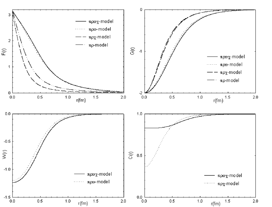
Figure 1: Profile functions - $F(r)$, $G(r)$, $W(r)$ and $C(r)$.

How does the dilaton affect this calculation? The $\pi\rho$ model with much smaller skyrmion has a larger baryon density near the origin and this affects the dilaton, significantly changing its mean-field value from its vacuum one. The net effect of the dilaton mean field on the mass is a reduction of $\sim$ 150 MeV, whereas for the $\pi\rho\omega$ model it is only of 50 MeV. The details can be seen in Table 2. The effect on the soliton size is, however, different: while the dilaton in the $\pi\rho$ model produces an additional localization of the baryon charge and hence reduces $\langle r^{2}\rangle$ from .21 fm² to .19 fm², in the $\pi\rho\omega$ model, on the contrary, the dilaton produces a $delocalization$ and increases $\langle r^{2}\rangle$ from .49 fm² to .51 fm².

In sum, we note that when the $\omega$ is present, it plays a major role in the skyrmion properties with the dilaton field playing a minor role.

Table 2: Single skyrmion mass and various contributions to it.

Model	$\langle r^{2}\rangle$	$E^{B=1}$	$E^{B=1}_{\pi}$	$E^{B=1}_{\pi\rho}$	$E^{B=1}_{\rho}$	$E^{B=1}_{\omega}$	$E^{B=1}_{WZ}$	$E^{B=1}_{\chi}$
$\pi\rho$-model	0.27	1054.6	400.2 + 9.2	110.4	534.9	0.0	0.0	0.0
$\pi\rho\chi$-model	0.19	906.5	103.1 + 1.4	155.1	504.1	0.0	0.0	142.8
$\pi\rho\omega$-model	0.49	1469.0	767.6 + 39.9	33.2	370.7	-257.6	515.1	0.0
$\pi\rho\omega\chi$-model	0.51	1408.3	646.0 + 29.2	34.9	355.7	-278.3	556.7	64.2

4 The B=2 Skyrmion : Product Ansatz

In the original Skyrme model with only pion fields, we can obtain a $B=2$ configuration by simply taking the product of two $B=1$ hedgehog $U$ fields. This configuration can be a good approximation to the true solution when the two skyrmions are sufficiently far apart. Furthermore the energy of this configuration becomes the lowest when one of the skyrmions is rotated in isospin space by an angle $\pi$ with respect to the axis perpendicular to the line joining two skyrmions. Here we have to generalize this feature to incorporate the $\rho$, $\omega$ and $\chi$ fields in the scheme. When two skyrmions are sufficiently far apart, our Ansatz should describe each individual skyrmion correctly. Recalling the field configurations for a single skyrmion at infinity, the most natural Ansatz is

$$\begin{array}[]{c}\displaystyle U_{B=2}\Leftarrow U_{B=1}(\vec{r}_{1})*U_{B=1}(\vec{r}_{2}),\\ \displaystyle\rho^{a,B=2}_{\mu}\Leftarrow\rho^{a,B=1}_{\mu}(\vec{r}_{1})+\rho^{a,B=1}_{\mu}(\vec{r}_{2}),\\ \displaystyle\omega^{B=2}_{\mu}\Leftarrow\omega^{B=1}_{\mu}(\vec{r}_{1})+\omega^{B=1}_{\mu}(\vec{r}_{2}),\\ \displaystyle\chi^{B=2}\Leftarrow\chi^{B=1}(\vec{r}_{1})*\chi^{B=1}(\vec{r}_{2}),\end{array}$$ (21)

where $\vec{r}_{1,2}$ stand for the position of the centers of each skyrmion. The boundary conditions for $B=1$ skyrmion imply that a multiplicative rule must apply to $U$ and $\chi$, since their vacuum values at infinity are 1, and an additive rule to $\rho$ and $\omega$, since theirs vanish at infinity.

The relative orientation takes place in isospin space. Thus the isoscalar fields, $\omega$ and $\chi$, do not undergo rotation. However the isovector fields $\pi$ and $\rho$ could require non-trivial relative orientations.

$$\begin{array}[]{c}\displaystyle U_{B=2}=U_{B=1}(\vec{r}_{1})*AU_{B=1}(\vec{r}_{2})A^{\dagger},\\ \\ \displaystyle\vec{\tau}\cdot\vec{\rho}^{B=2}_{\mu}=\vec{\tau}\cdot\vec{\rho}^{B=1}_{\mu}(\vec{r}_{1})+A\vec{\tau}\cdot\vec{\rho}^{a,B=1}_{\mu}(\vec{r}_{2})A^{\dagger},\end{array}$$ (22)

where $A$ is an SU(2) matrix. This Ansatz is a drastically simplified one and will not produce the lowest energy configuration of the $B=2$ system, known to be of the toroidal shape [13]. However for the purpose of our calculation, we need only the Ansatz defined by Eqs. (21) and (22), which will be used to define the starting configuration of the skyrmion matter [5]. As in the original Skyrme model, the lowest energy for this type of Ansatz can be obtained in the configuration where two skyrmions are relatively rotated in isospin space by an angle $\pi$ with respect to an axis perpendicular to the line joining them. (See Fig.2.)

In Fig.3, we show the density profile of the lowest energy configuration, in this approximation, which is of dumbbell shape with well-separated skyrmions.

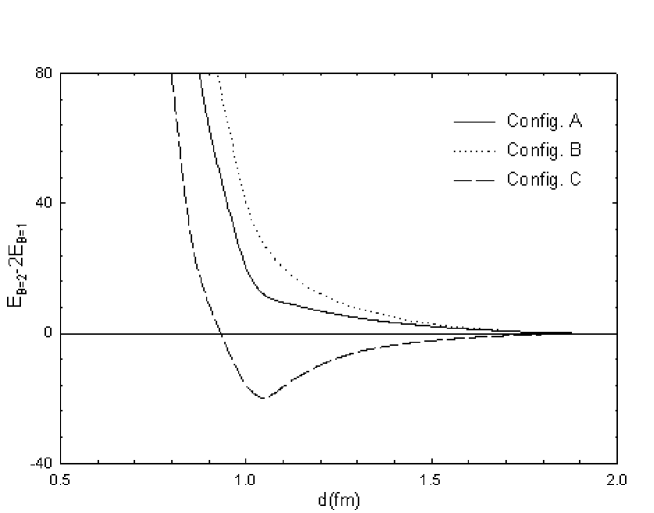
Figure 2: Binding energy of the two-skyrmion system. Configuration A represents the case with no relative rotation. Configuration B represents the case where the skyrmion is rotated by an angle $\pi/2$ with respect to the axis parallel to the line joining the two skyrmions. In configuration C, the angle is $\pi$ and the rotation axis is perpendicular to the line joining the two skyrmions.

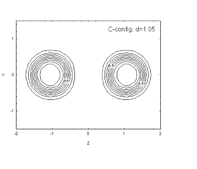
Figure 3: The lowest energy configuration obtained under the naive product Ansatz (21).

5 Skyrmion Matter : an FCC skyrmion crystal

We have learned from the study on two-skyrmion system in Sec.4 that the lowest-energy configuration is obtained when one of the skyrmions is rotated in isospin space with respect to the other by an angle $\pi$ about an axis perpendicular to the line joining the two. If we generalize this Ansatz to many-skyrmion matter, we obtain that the configuration at the classical level for a given baryon number density is an FCC crystal where the nearest neighbor skyrmions are arranged to have the attractive relative orientations [5] . We next proceed to incorporate the vector mesons by generalizing Kugler’s Fourier series expansion method [18], developed for the original Skyrme model, to our $\pi\rho\omega\chi$-model. The symmetries of such FCC crystal configuration are summarized in Table 3. As for the $\rho$-fields, we find it more convenient to give the symmetries for the dual vector fields $\tilde{\rho}_{p}$ as defined in Table 3. Note: (i) $\tilde{\rho}_{a}(a=1,2,3)$ has the same symmetries as $\pi_{a}$; (ii) the isoscalar fields $\sigma$, $\omega_{0}$ and $\chi$ share the same symmetries. One can easily check the symmetries for $\rho^{a}_{i}$(or $\tilde{\rho}_{a}$) and $\omega_{0}$ by referring to the useful relations (11) and (12).

Table 3: Symmetries of the FCC skyrmion crystal

		$\begin{array}[]{c}\mbox{reflection}\\ \mbox{($yz$-plane)}\end{array}$	$\begin{array}[]{c}\mbox{3-fold axis}\\ \mbox{rotation}\end{array}$	$\begin{array}[]{c}\mbox{4-fold axis}\\ \mbox{($z$-axis) rot.}\end{array}$	translation
$(x,y,z)$	$\rightarrow$	$(-x,y,z)$	$(y,z,x)$	$(x,z,-y)$	$(x+L,y+L,z)$
$U=\sigma+i\vec{\tau}\cdot\vec{\pi}$	$\rightarrow$	$(\sigma,-\pi_{1},\pi_{2},\pi_{3})$	$(\sigma,\pi_{2},\pi_{3},\pi_{1})$	$(\sigma,\pi_{1},\pi_{3},-\pi_{2})$	$(\sigma,-\pi_{1},-\pi_{2},\pi_{3})$
$\rho^{a}_{i}\equiv\varepsilon_{aip}\tilde{\rho}_{p}$	$\rightarrow$	$(-\tilde{\rho}_{1},\tilde{\rho}_{2},\tilde{\rho}_{3})$	$(\tilde{\rho}_{2},\tilde{\rho}_{3},\tilde{\rho}_{1})$	$(\tilde{\rho}_{1},\tilde{\rho}_{3},-\tilde{\rho}_{2})$	$(-\tilde{\rho}_{1},-\tilde{\rho}_{2},\tilde{\rho}_{3})$
$\omega_{0},\chi$	$\rightarrow$	$\omega_{0},\chi$	$\omega_{0},\chi$	$\omega_{0},\chi$	$\omega_{0},\chi$

5.1 Fourier series expansion

We next generalize our work in ref.([5, 6]), following Kugler and Shtrikman[18], to the problem at hand by indicating the pertinent expansions for all the fields.

• The pion expansion:

  We obtain the pion fields $\phi^{\pi}_{\alpha}$ from the un-normalized fields $\bar{\phi}^{\pi}_{\alpha}$ which are expanded in Fourier series as

  $$\begin{array}[]{rcl}\bar{\phi}^{\pi}_{0}&=&\displaystyle\sum_{abc}\beta^{\pi}_{abc}\cos(\pi ax/L)\cos(\pi by/L)\cos(\pi cz/L),\\ \bar{\phi}^{\pi}_{1}&=&\displaystyle\sum_{hkl}\alpha^{\pi}_{hkl}\sin(\pi hx/L)\cos(\pi ky/L)\cos(\pi lz/L),\\ \bar{\phi}^{\pi}_{2}&=&\displaystyle\sum_{hkl}\alpha^{\pi}_{hkl}\cos(\pi lx/L)\sin(\pi hy/L)\cos(\pi kz/L),\\ \bar{\phi}^{\pi}_{3}&=&\displaystyle\sum_{hkl}\alpha^{\pi}_{hkl}\cos(\pi kx/L)\cos(\pi ly/L)\sin(\pi hz/L),\end{array}$$ (23)

  and thereafter normalized

  $$\phi^{\pi}_{\alpha}=\frac{\bar{\phi}^{\pi}_{\alpha}}{\sqrt{\sum_{\beta}(\bar{\phi}^{\pi}_{\beta})^{2}}}.$$ (24)

  In order to be consistent with the symmetry properties listed in Table 3, $(a,b,c)$ should be all even or all odd integers, and $(k,l)$ should be all even(odd) if $h$ is odd(even). Furthermore, to provide a correct topological structure to the configuration, the expansion coefficients $\beta_{abc}$ must satisfy the constraint,

  $$\sum_{\mbox{\scriptsize even}}\beta^{\pi}_{abc}=0.$$ (25)

• The $\rho$ expansion :

  We introduce $\phi^{\rho}_{\alpha}(\alpha=0,1,2,3)$ and using Eq.(11), we may express $\rho^{a}_{i}$ in terms of these fields

  $$\rho^{a}_{i}=\varepsilon_{abc}\hat{\phi}^{\rho}_{b}\partial_{i}\hat{\phi}^{\rho}_{c}(1-\phi^{\rho}_{0})=\varepsilon_{abc}{\phi}^{\rho}_{b}\partial_{i}{\phi}^{\rho}_{c}/(1+\phi^{\rho}_{0}),$$ (26)

  where $\hat{\phi}^{\rho}_{a}=\phi^{\rho}_{a}/\sqrt{\sum_{b=1}^{3}(\phi^{\rho}_{b})^{2}}=\phi^{\rho}_{a}/\sqrt{1-(\phi^{\rho}_{0})^{2}}$. Similarly to the pion fields, $\phi^{\rho}_{\alpha}$ is obtained from the un-normalized fields $\bar{\phi}^{\rho}_{\alpha}$ whose expansion in Fourier series is

  $$\begin{array}[]{rcl}\bar{\phi}^{\rho}_{0}&=&\displaystyle\sum_{abc}\beta^{\rho}_{abc}\cos(\pi ax/L)\cos(\pi by/L)\cos(\pi cz/L),\\ \bar{\phi}^{\rho}_{1}&=&\displaystyle\sum_{hkl}\alpha^{\rho}_{hkl}\sin(\pi hx/L)\cos(\pi ky/L)\cos(\pi lz/L),\\ \bar{\phi}^{\rho}_{2}&=&\displaystyle\sum_{hkl}\alpha^{\rho}_{hkl}\cos(\pi lx/L)\sin(\pi hy/L)\cos(\pi kz/L),\\ \bar{\phi}^{\rho}_{3}&=&\displaystyle\sum_{hkl}\alpha^{\rho}_{hkl}\cos(\pi kx/L)\cos(\pi ly/L)\sin(\pi hz/L),\end{array}$$ (27)

  which we then normalize. The procedure is analogous to that of the pion fields, although the expansion coefficients are different.

• The $\omega$ and $\chi$ expansions :

  The isoscalar fields $\omega_{0}$ and $\chi$ have the same symmetry properties as the $\sigma$ and therefore their expansions are,

  $$\begin{array}[]{rcl}\omega_{0}/f_{\pi}\equiv w&=&\displaystyle\sum_{abc}\beta^{\omega}_{abc}\cos(\pi ax/L)\cos(\pi by/L)\cos(\pi cz/L),\\ \chi/f_{\chi}\equiv c&=&\displaystyle\sum_{abc}\beta^{\chi}_{abc}\cos(\pi ax/L)\cos(\pi by/L)\cos(\pi cz/L).\\ \end{array}$$ (28)

The expansion coefficients are determined such that the energy per skyrmion is minimized:

$$E/B=(E/B)_{\pi}+(E/B)_{\pi\rho}+(E/B)_{\rho}+(E/B)_{\omega}+(E/B)_{WZ}+(E/B)_{\chi}.$$ (29)

where

$$(E/B)_{\pi}=\textstyle\frac{1}{4}\displaystyle\int_{\mbox{\scriptsize Box}}d^{3}x\frac{f_{\pi}^{2}}{2}c^{2}\left\{(\partial_{i}\phi^{\pi}_{\alpha})^{2}+2m_{\pi}^{2}c(1-\phi^{\pi}_{0})\right\},$$

$$(E/B)_{\pi\rho}=\textstyle\frac{1}{4}\displaystyle\int_{\mbox{\scriptsize Box}}d^{3}x2f_{\pi}^{2}c^{2}\left\{\frac{\vec{\phi}^{\pi}\times\partial_{i}\vec{\phi}^{\pi}}{1+\phi^{\pi}_{0}}-\frac{\vec{\phi}^{\rho}\times\partial_{i}\vec{\phi}^{\rho}}{1+\phi^{\rho}_{0}}\right\}^{2},$$

$$(E/B)_{\rho}=\textstyle\frac{1}{4}\displaystyle\int_{\mbox{\scriptsize Box}}d^{3}x\frac{1}{8g^{2}}\left(\partial_{i}\phi^{\rho}_{\alpha}\partial_{j}\phi^{\rho}_{\beta}-\partial_{j}\phi^{\rho}_{\alpha}\partial_{i}\phi^{\rho}_{\beta}\right)^{2},$$

$$(E/B)_{\omega}=-\textstyle\frac{1}{4}\displaystyle\int_{\mbox{\scriptsize Box}}d^{3}x\textstyle\frac{1}{2}\left\{(\partial_{i}w_{0})^{2}+m_{\omega}^{2}c^{2}w_{0}^{2}\right\},$$

$$(E/B)_{WZ}=\textstyle\frac{1}{4}\displaystyle\int_{\mbox{\scriptsize Box}}d^{3}x\frac{3g}{2}f_{\pi}w_{0}B_{0},$$

$$(E/B)_{\chi}=\textstyle\frac{1}{4}\displaystyle\int_{\mbox{\scriptsize Box}}d^{3}x\frac{f_{\chi}^{2}}{2}\left\{(\partial_{i}c)^{2}+\textstyle\frac{1}{2}m_{\chi}^{2}[c^{4}(\ln c-\frac{1}{4})+\frac{1}{4}]\right\},$$

and

$$B_{0}=\frac{1}{12\pi^{2}}\varepsilon_{ijk}\varepsilon_{\alpha\beta\gamma\delta}\phi^{\pi}_{\alpha}\partial_{i}\phi^{\pi}_{\beta}\partial_{j}\phi^{\pi}_{\gamma}\partial_{k}\phi^{\pi}_{\delta}=\frac{1}{2\pi^{2}}\left|\begin{array}[]{cccc}\phi^{\pi}_{0}&\phi^{\pi}_{1}&\phi^{\pi}_{2}&\phi^{\pi}_{3}\\ \partial_{1}\phi^{\pi}_{0}&\partial_{1}\phi^{\pi}_{1}&\partial_{1}\phi^{\pi}_{2}&\partial_{1}\phi^{\pi}_{3}\\ \partial_{2}\phi^{\pi}_{0}&\partial_{2}\phi^{\pi}_{1}&\partial_{2}\phi^{\pi}_{2}&\partial_{2}\phi^{\pi}_{3}\\ \partial_{3}\phi^{\pi}_{0}&\partial_{3}\phi^{\pi}_{1}&\partial_{3}\phi^{\pi}_{2}&\partial_{3}\phi^{\pi}_{3}\end{array}\right|.$$

Since there are no constraints on the expansion parameters for the $\omega$ and $\chi$, a straightforward variational process of minimizing the energy fails. Note that as far as the energy of the system (29) is concerned, $\omega_{0}=0$ comes out as the solution which minimizes the energy . This is confirmed in Table 1 where we see that without the repulsive $\omega$, the single skyrmion mass becomes much lower. Therefore, the variational process always leads us to $w_{0}=0$, which corresponds to the energy per baryon of the $\pi\rho\chi$ model and not of the present model.

We realize that the $\omega$ needs a careful treatment in the model that incorporates it self-consistently. We proceed therefore to treat the $\omega$ in a more elaborate way. Instead of including the expansion coefficients $\beta^{\omega}_{abc}$ into the minimization process, we fix them by solving the equation of motion for $w(=w_{0}/f_{\pi})$ at each step. The equation of motion derived from (29) becomes

$$(-\partial_{i}^{2}+m_{\omega}^{2}c^{2})w=-\frac{3g}{2f^{2}_{\pi}}B_{0}.$$ (30)

Note that $c^{2}$ and $B_{0}$ have the same symmetry structure. Explicitly, the expansions (23) and (28) lead to

$$c^{2}=\sum_{abc}\beta^{c^{2}}_{abc}\cos(\pi ax/L)\cos(\pi by/L)\cos(\pi cz/L),$$ (31)

$$B_{0}=\sum_{abc}\beta^{B_{0}}_{abc}\cos(\pi ax/L)\cos(\pi by/L)\cos(\pi cz/L),$$ (32)

with the expansion coefficients $\beta^{c^{2}}_{abc}$ and $\beta^{B_{0}}_{abc}$ determined from the configuration of $\phi^{\pi}_{\alpha}$ and $c$. The equation of motion, therefore, reduces to a linear equation for the expansion coefficients $\beta^{\omega}_{abc}$ given by

$$\sum_{a^{\prime}b^{\prime}c^{\prime}}M_{abc,a^{\prime}b^{\prime}c^{\prime}}\beta^{\omega}_{a^{\prime}b^{\prime}c^{\prime}}=\frac{3g}{2f_{\pi}^{2}}\beta^{B_{0}}_{abc}.$$ (33)

The matrix elements are

$$M_{abc,a^{\prime}b^{\prime}c^{\prime}}=(a^{2}+b^{2}+c^{2})\left(\frac{\pi}{L}\right)^{2}\delta_{abc,a^{\prime}b^{\prime}c^{\prime}}+m^{2}_{\omega}\sum_{a^{\prime\prime}b^{\prime\prime}c^{\prime\prime}}\beta^{c^{2}}_{a^{\prime\prime}b^{\prime\prime}c^{\prime\prime}}f_{a^{\prime},a^{\prime\prime},a}f_{b^{\prime},b^{\prime\prime},b}f_{c^{\prime},c^{\prime\prime},c},$$ (34)

where

$$f_{a^{\prime},a^{\prime\prime},a}=\left\{\begin{array}[]{ll}\delta_{a^{\prime},a},&\mbox{if $a^{\prime\prime}=0$},\\ \delta_{a^{\prime\prime},a},&\mbox{if $a^{\prime}=0$},\\ \frac{1}{2}\delta_{a,a^{\prime}\pm a^{\prime\prime}},&\mbox{if $a^{\prime}\neq 0$ and $a^{\prime\prime}\neq 0$}.\end{array}\right.$$

As formulated, our variational procedure is restricted to evolve in the space of parameters which satisfy the $\omega$ equations of motion and therefore the “false” solution is not present in the scheme.

6 Results

We show in Figs. 4 and 5 the the numerical results of the energy per baryon $E/B$, $\langle\chi\rangle$ and $\langle\sigma\rangle$ in various models as a function of the FCC lattice parameter $L$ .

In the $\pi\rho\chi$ model, as the density of the system increases ($L$ decreases), $E/B$ changes little (see Fig. 4). It is close to the energy of a $B=1$ skyrmion up to a density greater than $\rho_{0}\;(L\sim 1.43)$. This result is easy to interpret. As we discussed in Sec. 3, the size of the skyrmion in this model is very small and therefore the skyrmions in the lattice will interact only at very high densities, high enough for their tails to overlap.

In the absence of the $\omega$, the dilaton field plays a dramatic role. A skyrmion matter undergoes an abrupt phase transition at high density at which the expectation value of the dilaton field vanishes $\langle\chi\rangle=0$ .

In the $\pi\rho\omega\chi$ model, the situation changes dramatically as can be seen in Fig.5. The reason is that the $\omega$ provides not only a strong repulsion among the skyrmions, but somewhat surprisingly, also an intermediate range attraction. Note the different mass scales between Figs. 4 and 5. In both the $\pi\rho\omega$ and the $\pi\rho\omega\chi$ models, at high density, the interaction reduces $E/B$ to 85% of the $B=1$ skyrmion mass. This value should be compared with 94% in the $\pi\rho$ model. In the $\pi\rho\chi$-model, $E/B$ goes down to 74% of the $B=1$ skyrmion mass, but in this case it is due to the dramatic behavior of the dilaton field.

In the $\pi\rho\omega\chi$ model the role of the dilaton field is suppressed. It provides a only a small attraction at intermediate densities. Moreover, the phase transition towards its vanishing expectation value, $\langle\chi\rangle=0$, does not take place. Instead, its value grows at high density!

In all the models analyzed thus far, $\langle\sigma\rangle$ goes to zero at high density. Thus, we have two different scenarios for the chiral transition. The models without the $\omega$, but with $\chi$, tend to bring about a phase transition that is consistent with the “vector manifestation” scenario, with the pion decay constant $f_{\pi}$ vanishing. However, once the $\omega$ is present, the $f_{\pi}$ remains non-zero while $\langle\sigma\rangle$ vanishes, a scenario that is reminiscent of the pseudo-gap realization. This is at variance with the VM scenario.

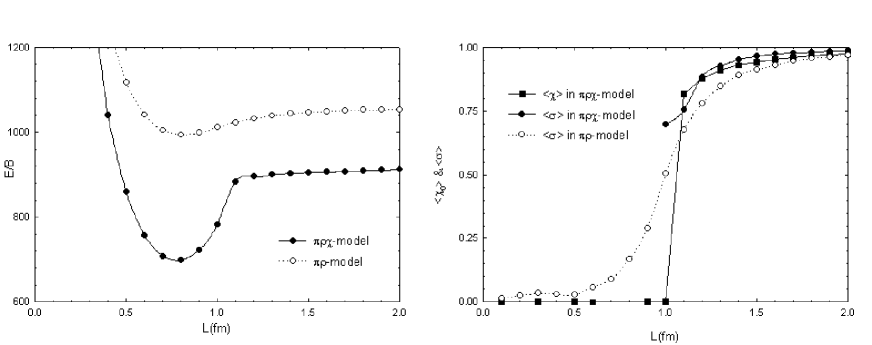
Figure 4: $E/B$, $\langle\chi\rangle$ and $\langle\sigma\rangle$ as a function of $L$ in the models without the $\omega$.

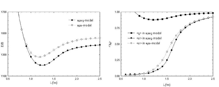
Figure 5: $E/B$, $\langle\chi\rangle$ and $\langle\sigma\rangle$ as a function of $L$ in the models with the $\omega$.

Let us discuss in detail why and how the $\omega$ changes the VM-like behavior of the $\pi\rho\chi$ model at the phase transition into a pseudo-gap scenario. The term in the Lagrangian responsible for this behavior is the coupling of the $\omega$ to the topological current $B_{0}$, i.e. Eqs.(29.e) and (29.g). To see this point, we write the equation of motion for the $\omega$ as

$$(-\partial_{i}^{2}+m_{\omega}^{*2})w=-\frac{3g}{2f_{\pi}^{2}}B_{0},$$

where we have replaced the space-dependent mass term $m_{\omega}^{2}c^{2}$ of Eq.(30) by an effective mass $m_{\omega}^{*2}$. This equation can be exactly solved by means of the appropriate Green’s function,

$$w=-\frac{3g}{2f_{\pi}^{2}}\int d^{3}x^{\prime}\frac{\exp(-m_{\omega}^{*}|\vec{x}-\vec{x}^{\prime}|)}{4\pi|\vec{x}-\vec{x}^{\prime}|}B_{0}(\vec{r^{\prime}}).$$ (35)

Thus, $w$ can be interpreted as a static potential generated by the source $B_{0}$. The $\omega$ contribution to $E/B$ can be expressed as

$$(E/B)_{WZ}=\textstyle\frac{1}{4}\displaystyle\int_{\mbox{\scriptsize Box}}d^{3}x\int d^{3}x^{\prime}\left(\frac{3g}{2}\right)^{2}B_{0}(\vec{x})\frac{\exp(-m_{\omega}^{*}|\vec{x}-\vec{x}^{\prime}|)}{4\pi|\vec{x}-\vec{x}^{\prime}|}B_{0}(\vec{x}^{\prime}),$$ (36)

and the term $(E/B)_{\omega}$ is, as mentioned previously, $-\frac{1}{2}$ of this. Note that while the integral over $\vec{x}$ is defined in a single FCC cell, that over $\vec{x}^{\prime}$ is not. Thus, unless it is screened, the periodic source $B_{0}$ filling infinite space will produce an infinite potential $w$ which leads to an infinite $(E/B)_{WZ}$. The screening is done by the omega mass, $m_{\omega}^{*}$, as can be seen from Eq.(36). Thus the effective $\omega$ mass cannot vanish for the solution! Our numerical results reflect this fact: at high density the $B_{0}$-$B_{0}$ interaction becomes large compared to any other contribution. In order to reduce it, $\chi$ has to increase, and thereby the effective screening mass $m_{\omega}^{*}\sim m_{\omega}\langle\chi\rangle$ becomes larger. In this way we run into a phase transition where the expectation value of $\chi$ does not vanish and therefore $f_{\pi}$ does not vanish but instead increases.

7 Concluding remarks

This paper represents the natural continuation of our effort to understand the physics of nuclear matter from the Skyrme model description. The (original) Skyrme model is an effective theory which represents the large $N_{c}$ limit of $QCD$. In some sense, it is the lowest order of a bosonized approach to this theory. Higher orders will be obtained by incorporating massive mesons. In particular, we know from phenomenology that the vector mesons play a crucial role in describing the N-N interaction [19] and infinite nuclear matter [9]. Thus going beyond our previous developments [5, 6], the next natural step is to implement vector mesons in consistency with $QCD$ [20, 21]. The model we studied in this paper contains, in addition to the Goldstone pions, the scale dilaton associated with trace anomaly of QCD and the $\rho$ and $\omega$ fields introduced according to the hidden local symmetry strategy.

As in our previous work without vector mesons, the skyrmion matter possesses two phases: a low-density phase which we simply describe here by an FCC crystal and a high-density phase which is described by a half-skyrmion CC crystal. In our previous work, the dilaton was crucial to realize the phase transition in a scenario consistent with the vector manifestation (VM) fixed point structure: The phase transition was signalled by the vanishing of both $\langle\sigma\rangle$ and $f_{\pi}^{*}$. However in the present model with the vector mesons, in particular with the $\omega$, the mean $\chi$ field cannot vanish and therefore, although $\langle\sigma\rangle$ vanishes, $f_{\pi}^{*}$ does not and we seem to fall back to a pseudo-gap-type of picture which does not seem consistent with the VM and in that matter with the standard sigma-model scenario. The sole agent responsible for this puzzling feature is the $\omega$ meson.

If the $\omega$ is not present, i.e., in the $\pi\rho\chi$ model, the behavior is the conventional one. The $\chi$ field vanishes at the phase transition and chiral restoration is produced in the standard scenario. The $\rho$ meson is basically a spectator at the classical level, producing little change with respect to our previously studied $\pi\chi$ model [6, 7] except that at high densities, once the $\rho$ starts to overlap, the energy of nuclear matter increases due to its the repulsive effect at short distances. The densities have to be quite high since these skyrmions are very small. Since $\chi$ vanishes at the phase transition, we recover the VM behavior, namely, $f_{\pi}^{*}=0$ and $m_{\rho}^{*}=0$.

The incorporation of the $\omega$ changes dramatically the scales. Since the $\omega$ produces a strong repulsion, the skyrmions become more massive and much bigger in size [8]. Moreover the phase transition scenario changes dramatically from the previously described. In particular, $\chi$ does not vanish at the phase transition but it even increases its value. The mechanism of how this happens is simple and robust. It is that the $\omega$ coupling to the baryon density in our scheme leads in nuclear matter to a long range infinite interaction unless some sort of screening intervenes. However in medium the effective $\omega$ mass becomes $m_{\omega}^{*}=m_{\omega}\chi$. Thus if $\chi$ decreases, the effective mass decreases and the screening decreases, thus the long-range interaction becomes stronger and ultimately will tend to dominate. In order to prevent this from happening, the background skyrmion counteracts so as to compensate for the increase in the baryon density interaction: It increases the value of the $\chi$ field and hence the effective $\omega$ mass, i.e., the screening. Since the in-medium value of the pion decay constant is locked to the mean-field value of $\chi$ which does not vanish at the chiral transition, $f_{\pi}$ does not vanish, whereas the $\langle\sigma\rangle$, whose vanishing is linked to the structure of the crystal, does to vanish at the critical point, signalling the phase transition as in our naive scenario [5].

The qualitatively dramatic effect of the $\omega$ meson in the skyrmion structure of dense matter is at the same time disturbing and puzzling. In nuclear physics, $\omega$ has been a crucial element [9], so it makes one wonder what goes wrong at densities greater than that of normal nuclear matter. We have no clear answer at this point but we can think of three possibilities: (a) the minimal Lagrangian we use is inadequate in that short-distance physics is not $fully$ accounted for. Since the $\omega$ degree of freedom accounts for nuclear interactions at short distance, higher derivatives and/or higher-dimension operators could be indispensable; (b) the Wilsonian matching of effective field theories to QCD as discussed by Harada and Yamawaki [2] requires that the parameters of the effective theory be $intrinsically$ density- and temperature-dependent. This would mean that the coupling constants – and not just the masses of the vector mesons – will have $intrinsic$ dependence which may not be fully accounted for by the response to the background skyrmion matter that is taken into account in our model. This feature was noted already at nuclear matter density [22, 4] where the $\omega$ coupling was found to decrease along with the BR scaling mass of the $\omega$ in order to obtain the saturation and binding of nuclear matter; (c) in describing dense matter approaching chiral restoration in terms of $explicit$ (as opposed to integrated-out) massive degrees of freedom, the lowest-lying vector mesons may not be sufficient. It may be that the tower of vector mesons as suggested in the “open moose” model of Son and Stephanov [23] – which is conjectured to be dual to QCD – may have to be implemented consistently with the symmetries of QCD. These points are being investigated and will be reported in future publications.

References

- [1] M. Harada and K. Yamawaki, Phys. Rev. Lett. 86 (2001) 757.
- [2] For an extensieve review, see M. Harada and K. Yamawaki, Phys. Rep. 381 (2003) 1.
- [3] G.E. Brown and M. Rho, Phys. Rev. Lett 66 (1991) 2720.
- [4] G.E. Brown and M. Rho, Phys. Rept. 363 (2002) 85; nucl-th/0206021, nucl-th/0305089.
- [5] H.-J. Lee, B.-Y. Park, D.-P. Min, M. Rho and V. Vento, Nucl.Phys. A723 (2003) 427.
- [6] H.-J. Lee, B.-Y. Park, M. Rho and V. Vento, Nucl.Phys. A726 (2003) 69.
- [7] H.-J. Lee, B.-Y. Park, M. Rho and V. Vento, “The Pion Velocity in Dense Skyrmion Matter”, hep-ph/0307111.
- [8] I. Zahed and G.E. Brown, Phys. Rep. 142 (1986) 1; Ulf.-G. Meißner, Phys. Rep. 161 (1988) 213.
- [9] B.D. Serot and J.D. Walecka, Adv. Nucl. Phys. 16 (1986) 1.
- [10] J. Ellis and J. Lanik, Phys. Lett. B150 (1985) 289.
- [11] M. Bando, T. Kugo and K. Yamawaki, Phys. Rep. 164 (1988) 217.
- [12] Ulf-G. Meißner, A.Rakhimov, U. Yakhshiev, Phys. Lett. B473 (2000) 200.
- [13] R.A. Leese, N.S. Manton, B.J. Schroers, Nucl.Phys. B442(1995)228.
- [14] L. Pauling, Phys. Rev. Lett. 15 (1965) 499; N.D. Cook and V. Dallacasa, Phys. Rev. C35 (1987) 1883; N.D. Cook, J. Phys. G: Nucl. Part. Phys. 20 (1994) 1907.
- [15] J. Garai, nucl-th/0309035.
- [16] T. Goldman, G.J. Stephenson, Kim Maltman and K.E. Schmidt, Nucl. Phys. 481 (1988) 621.
- [17] Kim Maltman, G.J. Stephenson and T. Goldman, Phys. Lett. B 324 (1994) 1.
- [18] M. Kugler and S. Shtrikman, Phys. Lett. B208 (1988) 491; Phys. Rev. D40 (1989) 3421.
- [19] A.D. Jackson and G.E. Brown, The Nucleon-Nucleon interaction (North Holland, Amsterdam 1976).
- [20] S. Weinberg, Physica 96A (1979) 327.
- [21] E. Witten, Nucl. Phys. 223 (1983) 422.
- [22] C. Song, Phys. Rep. 347 (2001) 289.
- [23] D.T. Son and M.A. Stephanov, “QCD and dimensional reduction,” hep-ph/0304182.