Connecting Polyakov Loops to Hadrons

Abstract

The order parameter for the pure Yang-Mills phase transition is the Polyakov loop, which encodes the symmetries of the $Z_{N}$ center of the $SU(N)$ gauge group. The physical degrees of freedom of any asymptotically free gauge theory are hadronic states. Using the Yang-Mills trace anomaly and the exact $Z_{N}$ symmetry we show that the transfer of information from the order parameter to hadrons is complete.

1 Introduction

Recently in [1, 2, 3, 4] we have analyzed the problem of how, and to what extent the information encoded in the order parameter of a generic theory is transferred to the non-order parameter fields. This is a fundamental problem since in nature most fields are non-order parameter fields.

This problem is especially relevant in QCD and QCD-like theories since there is no physical observable for deconfinement which is directly linked to the order parameter field. Here we mainly review the first work [1] on this issue, which deals with the confinement/deconfinement phase transition in pure Yang-Mills theory.

Importance sampling lattice simulations are able to provide vital information about the nature of the temperature driven phase transition for 2 and 3 color Yang-Mills theories with and without matter fields (see [5, 6] for 3 colors). At zero temperature the $SU(N)$ Yang-Mills theory is asymptotically free, and the physical spectrum of the theory consists of a tower of hadronic states referred to as glueballs and pseudo-scalar glueballs. The theory develops a mass gap and the lightest glueball has a mass of the order of few times the confining scale. The classical theory possesses conformal symmetry, while quantum corrections lead to a non-vanishing trace of the energy momentum tensor.

At nonzero temperature the $Z_{N}$ center of $SU(N)$ is a relevant global symmetry [7], and it is possible to construct a number of gauge invariant operators charged under $Z_{N}$. Among these the most notable one is the Polyakov loop:

$${\ell}\left(x\right)=\frac{1}{N}{\rm Tr}[{\bf L}]\equiv\frac{1}{N}{\rm Tr}\left[{\cal P}\exp\left[i\,g\int_{0}^{1/T}A_{0}(x,\tau)d\tau\right]\right]$$

${\cal P}$ denotes path ordering, $g$ is the $SU(N)$ coupling constant, $x$ is the coordinate for the three spatial dimensions, and $\tau$ is the Euclidean time. The $\ell$ field is real for $N=2$, while otherwise complex. This object is charged with respect to the center $Z_{N}$ of the $SU(N)$ gauge group [7], under which it transforms as $\ell\rightarrow z\ell$ with $z\in Z_{N}$. A relevant feature of the Polyakov loop is that its expectation value vanishes in the low temperature regime, and is non-zero in the high temperature phase. The Polyakov loop is thus a suitable order parameter for the Yang-Mills temperature driven phase transition [7].

Here we consider pure gluon dynamics. This allows us to have a well defined framework where the $Z_{N}$ symmetry is exact. The hadronic states are the glueball fields ($H$) and their effective theory at the tree level is constrained by the Yang-Mills trace anomaly.

A puzzle is how the information about the Yang-Mills phase transition encoded, for example, in the $Z_{N}$ global symmetry can be communicated to the hadronic states of the theory. Here we propose a concrete way to resolve the puzzle.

As basic ingredients we use the trace anomaly and the $Z_{N}$ symmetry. They will be enough to demonstrate that the information carried by $\ell$ is efficiently and completely transferred to the glueballs. More generally, the glueball field is a function of $\ell$:

$$H\equiv H[\ell].$$ (1)

Our results can be tested via first principle lattice simulations.

2 The Basic Properties

The hadronic states of the Yang-Mills theory are the glueballs. At zero temperature the Yang-Mills trace anomaly has been used to constrain the potential of the lightest glueball state $H$ [9]:

$$V[H]=\frac{H}{2}\ln\left[\frac{H}{\Lambda^{4}}\right].$$ (2)

$\Lambda$ is chosen to be the confining scale of the theory and $H$ is a mass dimension four field. This potential correctly saturates the trace anomaly when $H$ is assumed to be proportional to ${\rm Tr}\left[G_{\mu\nu}G^{\mu\nu}\right]$ and $G_{\mu\nu}$ is the standard Yang-Mills field strength. The potential nicely encodes the properties of the Yang-Mills vacuum at zero temperature and it has been used to deduce a number of phenomenological results [9]. Effective Lagrangians play a relevant role for describing strong dynamics. Recently, for example a number of fundamental results at zero temperature and matter density about the vacuum properties and spectrum of QCD have been uncovered [10].

At high temperature the Yang-Mills pressure can be written in terms of the field $\ell$ according to the Polyakov Loop Model (PLM) of [8]. This free energy must be invariant under $Z_{N}$ and it takes the general form:

$$V[\ell]=T^{4}{\cal F}[\ell].$$ (3)

${\cal F}[\ell]$ is a polynomial in $\ell$ invariant under $Z_{N}$, and its coefficients depend on the temperature, allowing for a mean field description of the Yang-Mills phase transitions.

We now marry the two models by requiring both fields to be present simultaneously at non zero temperature. The theory must reproduce the ordinary glueball Lagrangian at low temperatures and the PLM Lagrangian at high temperatures. In [1] the following effective potential was proposed:

$$V\left[H,\ell\right]=\frac{H}{2}\ln\left[\frac{H}{\Lambda^{4}}\right]+V_{T}\left[H\right]+H{\cal P}{\left[\ell\right]}+T^{4}{\cal V}\left[\ell\right],$$ (4)

where ${\cal V}\left[\ell\right]$ and ${\cal P}\left[\ell\right]$ are general (but real) polynomials in $\ell$ invariant under $Z_{N}$ whose coefficients depend on the temperature. The explicit dependence is not known and should be fit to lattice data. Dimensional analysis and analyticity in $H$ when coupling it with $\ell$ severely restricts the effective potential terms. We stress that $H{\cal P}[\ell]$ is the most general interaction term which can be constructed without spoiling the zero temperature trace anomaly. Further nonanalytic interaction terms can arise when considering thermal and quantum corrections. These are partially contained in $V_{T}[H]$ which schematically represents the temperature of a gas of glueballs. In the following we will not investigate in detail such a term. Our theory cannot be the full story since we neglected (as customary) all of the tower of glueballs and pseudo-scalar glueballs as well as the infinite series of dimensionless gauge invariant operators with different charges with respect to $Z_{N}$. Nevertheless, the potential is sufficiently general to capture the essential features of the Yang-Mills phase transition.

When the temperature $T$ is much less than the confining scale $\Lambda$ the last term in Eq. (4) can be safely neglected. Since the glueballs are relatively heavy compared to the $\Lambda$ scale their temperature contribution $V_{T}[H]$ can also be disregarded. At low temperatures the theory reduces to the standard glueball potential augmented by the third term which does not affect the trace anomaly.

At very high temperatures (compared to $\Lambda$) the last term dominates ($H$ itself is very small) recovering the picture in which $\ell$ dominates the free energy. In this regime we have ${\cal F}[\ell]={\cal V}[\ell]$.

We can, in principle, compute all the relevant thermodynamic quantities in our approach, i.e. entropy, pressure etc., but this is not the main scope of this work.

A relevant object is the trace of the energy-momentum tensor $\Theta^{\mu}_{\mu}$. At zero temperature, and when the potential is a general function of a set of bosonic fields $\{\Phi_{n}\}$ with mass-dimensions $d_{n}$, one can construct the associated trace of the energy-momentum tensor via:

$$\Theta^{\mu}_{\mu}=4V[\Phi_{n}]-\sum_{n}\frac{\delta V[\Phi_{n}]}{\delta\Phi_{n}}\Phi_{n}\,d_{n}.$$ (5)

At finite temperature we still define our temperature dependent energy-momentum tensor as in Eq. (5). Here $H$ possesses engineering mass dimensions $4$ while $\ell$ is dimensionless, yielding the following temperature dependent stress energy tensor:

$$\Theta^{\mu}_{\mu}(T)=-2H+4T^{4}{\cal V}[\ell]+4\left[1-H\frac{\delta}{\delta H}\right]V_{T}[H].$$ (6)

$\Theta^{\mu}_{\mu}$ is normalized such that $\langle 0|\Theta^{\mu}_{\mu}|0\rangle=\epsilon-3p$ with $\epsilon$ the vacuum energy density and $p$ the pressure. At zero temperature only the first term survives, yielding magnetic type condensation typical of a confining phase, while at extremely high temperature the second term dominates, displaying an energy density and a pressure typical of a deconfined phase.

The theory containing just $\ell$ can be obtained integrating out $H$ via the equation of motion:

$$\frac{\delta V[H,\ell]}{\delta H}=0\,.$$ (7)

Formally this is justifiable if the glueball degrees of freedom are very heavy. For simplicity we neglect the contribution of $V_{T}[H]$, as well as the mean-field theory corrections for $\ell$. However, a more careful treatment which also includes the kinetic terms should be considered [2, 11]. Within these approximations the equation of motion yields:

$$H[\ell]=\frac{\Lambda^{4}}{e}\exp\left[-2{\cal P}[\ell]\right].$$ (8)

The previous expression shows the intimate relation between $\ell$ and the physical states of strongly interacting theories.

After substituting Eq. (8) back into the potential (4) and having neglected $V_{T}[H]$ we have:

$$V[\ell]=T^{4}{\cal V}[\ell]-\frac{\Lambda^{4}}{2e}\exp\left[-2{\cal P}[\ell]\right].$$ (9)

This formula shows that for large temperatures the only relevant energy scale is $T$ and we recover the PLM model. At low temperatures the scale $\Lambda$ allows for new terms in the Lagrangian. Besides the $T^{4}$ and the $\Lambda^{4}$ terms we also expect terms with coefficients of the type $T\Lambda^{3}$ and $T^{2}\Lambda^{2}$ and $T^{3}\Lambda$. However in our simple model these terms do not seem to emerge.

Expanding the exponential we have:

$$V[\ell]=T^{4}{\cal V}[\ell]+\frac{\Lambda^{4}}{e}{\cal P}[\ell]-\frac{\Lambda^{4}}{2e}+\cdots.$$ (10)

Since ${\cal V}[\ell]$ and ${\cal P}[\ell]$ are real polynomials in $\ell$ invariant under $Z_{N}$ we immediately recover a general potential in $\ell$.

3 The two Color Theory

To illustrate how our formalism works we first consider in detail the case $N=2$ and neglect for simplicity the term $V_{T}[H]$. This theory has been extensively studied via lattice simulations [12, 13] and it constitutes the natural playground to test our model. Here $\ell$ is a real field and the $Z_{2}$ invariant ${\cal V}[\ell]$ and ${\cal P}[\ell]$ are taken to be:

$${\cal V}\left[\ell\right] = a_{1}\ell^{2}+a_{2}\ell^{4}+{\cal O}(\ell^{6}),$$

$${\cal P}\left[\ell\right] = b_{1}\ell^{2}+{\cal O}(\ell^{4}),$$ (11)

with $a_{1},~{}a_{2}$ and $b_{1}$ unknown temperature dependent functions, which should be derived directly from the underlying theory. Lattice simulations can, in principle, fix all of the coefficients. In order for us to investigate in some more detail the features of our potential, and inspired by the PLM model mean-field type of approximation, we first assume $a_{2}$ and $b_{1}$ to be positive and temperature independent constants, while we model $a_{1}=\alpha(T_{\ast}-T)/T$, with $T_{\ast}$ a constant and $\alpha$ another positive constant. We will soon see that due to the interplay between the hadronic states and $\ell$, $T_{\ast}$ need not to be the critical Yang-Mills temperature while $a_{1}$ displays the typical behavior of the mass square term related to a second order type of phase transition.

The extrema are obtained by differentiating the potential with respect to $H$ and $\ell$:

$$\frac{\partial V}{\partial H} = \frac{\ln}{2}\left[\frac{eH}{\Lambda^{4}}\right]+{\cal P}\left[\ell\right]=\frac{\ln}{2}\left[\frac{eH}{\Lambda^{4}}\right]+b_{1}\ell^{2}=0$$ (12)

$$\frac{\partial V}{\partial\ell} = 2\ell T^{4}\left(a_{1}+\frac{H}{T^{4}}b_{1}+2a_{2}\ell^{2}\right)=0\,.$$ (13)

3.1 Small and Intermediate Temperatures

At small temperatures the second term in Eq. (13) dominates and the only solution is $\ell=0$. A vanishing $\ell$ leads to a null ${\cal P}[\ell]$ yielding the expected minimum for $H$:

$$\langle H\rangle=\frac{\Lambda^{4}}{e}.$$ (14)

Here $\ell$ and $H$ decouple.

We now study the solution near the critical temperature for the deconfinement transition. At all temperatures for which

$$T^{4}a_{1}+{H}b_{1}=T^{3}\alpha(T_{\ast}-T)+Hb_{1}>0,$$ (15)

the solution for $\ell$ is still $\ell=0$, yielding Eq. (14). The critical temperature is reached for

$$T_{c}=T_{\ast}+\frac{b_{1}}{e\alpha}\frac{\Lambda^{4}}{T_{c}^{3}}\,,$$ (16)

and can be determined via lattice simulations. We see that within our framework the latter is related to the glueball (gluon-condensate) coupling to two Polyakov loops and it would be relevant to measure it on the lattice. At $T=T_{c}$, $\ell=0$ and $H=\Lambda^{4}/e$.

Let us now consider the case $T=T_{c}+\Delta T$ with

$$\frac{\Delta T}{T_{c}}\ll 1.$$ (17)

Expanding $\langle\ell\rangle^{2}$ at the leading order in $\Delta T/T_{c}$ yields:

$$\langle\ell\rangle^{2}=\frac{\alpha}{2a_{2}}\frac{1+3\frac{b_{1}}{e\alpha}\frac{\Lambda^{4}}{T_{c}^{4}}}{1-\frac{b_{1}^{2}}{ea_{2}}\frac{\Lambda^{4}}{T_{c}^{4}}}\,\frac{\Delta T}{T_{c}}.$$ (18)

We used Eq. (16) and Eq. (12) which relates the temperature dependence of $H$ to the one of $\ell$. At high temperatures (see next subsection) $\langle\ell\rangle$ can be normalized to one by imposing $\alpha/2a_{2}=1$ and the previous expression reads:

$$\langle\ell\rangle^{2}=\frac{1+3\frac{b_{1}}{e\alpha}\frac{\Lambda^{4}}{T_{c}^{4}}}{1-\frac{2b_{1}^{2}}{e\alpha}\frac{\Lambda^{4}}{T_{c}^{4}}}\,\frac{\Delta T}{T_{c}}\equiv\frac{4T_{c}-3T_{\ast}}{(1-2b_{1})T_{c}+2b_{1}T_{\ast}}\,\frac{\Delta T}{T_{c}}.$$ (19)

For a given critical temperature consistency requires $b_{1}$ and $T_{\ast}$ to be such that:

$$\frac{4T_{c}-3T_{\ast}}{(1-2b_{1})T_{c}+2b_{1}T_{\ast}}\geq 0.$$ (20)

In this regime, the temperature dependence of the gluon condensate is:

$$\langle H\rangle=\frac{\Lambda^{4}}{e}\,\exp\left[-2b_{1}\langle\ell\rangle^{2}\right].$$ (21)

We find the mean field exponent for $\ell$, i.e. $\ell^{2}$ increases linearly with the temperature near the phase transition . Interestingly, the gluon-condensates drops exponentially. This drop is triggered by the rise of $\ell$ and it happens in our simple model exactly at the deconfining critical temperature. Although the drop might be sharp it is continuous in temperature. This is related to the fact that the phase transition is second order. Our findings strongly support the common picture according to which the drop of the gluon condensate signals, in absence of quarks, deconfinement.

3.2 High Temperature

At very high temperatures the second term in Eq. (13) can be neglected and the minimum for $\ell$ is:

$$\langle\ell\rangle=\sqrt{\frac{\alpha}{2a_{2}}}.$$ (22)

For $H$ we have now:

$$\langle H\rangle=\frac{\Lambda^{4}}{e}\exp\left[-2b_{1}\frac{\alpha}{2a_{2}}\right]=\frac{\Lambda^{4}}{e}\exp\left[-2b_{1}\right].$$ (23)

In the last step we normalized $\langle\ell\rangle$ to unity at high temperature. In order for the previous solutions to be valid we need to operate in the following temperature regime:

$$T\gg\sqrt[4]{\frac{b_{1}}{\alpha}{\langle H\rangle}}\approx T_{c}.$$ (24)

We find that at sufficiently high temperature $\langle H\rangle$ is exponentially suppressed and the suppression rate is determined solely by the glueball – $\ell^{2}$ mixing term encoded in ${\cal P}[\ell]$. The coefficient $b_{1}$ should be large (or increase with the temperature) since we expect a vanishing gluon-condensate at asymptotically high temperatures. Clearly it is crucial to determine all of these coefficients via first principle lattice simulations. The qualitative picture which emerges in our analysis is summarized in Fig. 1.

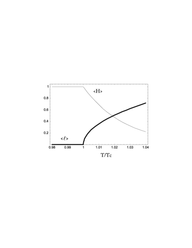
Figure 1: The thin line is the gluon condensate $\langle H\rangle$ normalized to $\Lambda^{4}/e$ as function of temperature. The thick line is $\langle\ell\rangle$ normalized to unity as function of temperature. We chose for illustration $\alpha=1$, $b_{1}=1.45$ and $T_{c}\simeq 1.16\Lambda$.

4 The three color theory

$Z_{3}$ is the global symmetry group for the three color case and $\ell$ is a complex field. The functions ${\cal V}[\ell]$ and ${\cal P}[\ell]$ are:

$${\cal V}\left[\ell\right] = a_{1}|\ell|^{2}+a_{2}|\ell|^{4}-a_{3}(\ell^{3}+{\ell^{\ast}}^{3})+{\cal O}(\ell^{5}),$$

$${\cal P}\left[\ell\right] = b_{1}|\ell|^{2}+{\cal O}(\ell^{3}),$$ (25)

with $a_{1}$, $a_{2}$, $a_{3}$ and $b_{1}$ unknown temperature dependent coefficients which can be determined using lattice data. Here we want to investigate the general relation between glueballs and $\ell$, so we will not try to find the best parameterization to fit the lattice data. In the spirit of the mean field theory we take $a_{2}$, $a_{3}$ and $b_{1}$ to be positive constants while $a_{1}=\alpha(T_{\ast}-T)/T$. With $\ell=|\ell|e^{i\varphi}$ the extrema are now obtained by differentiating the potential with respect to $H$, $|\ell|$ and $\varphi$:

$$\frac{\partial V}{\partial H} = \frac{\ln}{2}\left[\frac{eH}{\Lambda^{4}}\right]+{\cal P}\left[\ell\right]=\frac{\ln}{2}\left[\frac{eH}{\Lambda^{4}}\right]+b_{1}|\ell|^{2}=0$$

$$\frac{\partial V}{\partial|\ell|} = 2|\ell|T^{4}\left(a_{1}+\frac{H}{T^{4}}b_{1}-3a_{3}|\ell|\cos(3\varphi)+2a_{2}|\ell|^{2}\right)=0$$

$$\frac{\partial V}{\partial\varphi} = 6|\ell|^{3}\,\sin(3\varphi)=0\,.$$ (26)

At small temperature the $H/T^{4}$ term in the second equation dominates and the solution is $\langle|\ell|\rangle=0$, $\langle H\rangle=\Lambda^{4}/e$. The last equation is verified for any $\langle\varphi\rangle$, so we choose $\langle\varphi\rangle=0$. The second equation can have two more solutions:

$$\frac{3}{4}\frac{a_{3}}{a_{2}}\pm\sqrt{\frac{9}{16}\frac{a_{3}^{2}}{a_{2}^{2}}+\frac{\alpha(T-T_{\ast})}{2Ta_{2}}-\frac{b_{1}H}{2a_{2}T^{4}}},$$ (27)

whenever the square root is well defined, i.e. at sufficiently high temperatures. The negative sign corresponds to a relative maximum, while the positive one to a relative minimum. We have then to evaluate the free energy value (i.e. the effective thermal potential) at the relative minimum and compare it with the one at $\ell=0$. The temperature value for which the two minima have the same free energy is defined as the critical temperature and is:

$$T_{c}=\left[T_{\ast}+\frac{b_{1}}{e\alpha}\frac{\Lambda^{4}}{T_{c}^{3}}\right]\frac{\alpha a_{2}}{\alpha a_{2}+a_{3}^{2}}.$$ (28)

When $a_{3}$ vanishes we recover the second order type critical temperature. To derive the previous expression we held the value of $H$ fix to $\Lambda^{4}/e$ at the transition point. In a more refined treatment one should not make such an assumption. Below this temperature the minimum is still for $\langle\ell\rangle=0$ and $\langle H\rangle=\Lambda^{4}/e$. Just above the critical temperature the fields jump to the new values:

$$\langle|\ell|\rangle=\frac{a_{3}}{a_{2}},\qquad\langle H\rangle=\frac{\Lambda^{4}}{e}\exp{\left[-2b_{1}\langle|\ell|\rangle^{2}\right]}.$$ (29)

Close to, but above $T_{c}$ (i.e. $T=T_{c}+\Delta T$) we have:

$$\langle|\ell|\rangle\simeq\frac{a_{3}}{a_{2}}+\rho\frac{\Delta T}{T_{c}},$$ (30)

with

$$\rho \simeq \frac{\alpha a_{2}}{a_{3}}\frac{4\kappa T_{c}-3T_{\ast}}{a_{2}T_{c}-4b_{1}\alpha(\kappa T_{c}-T_{\ast})},$$

$$\kappa = \frac{\alpha a_{2}+a_{3}^{2}}{\alpha a_{2}}\,,$$ (31)

a positive function of the coefficients of the effective potential. In this regime

$$\langle H\rangle=\frac{\Lambda^{4}}{e}\exp\left[-2b_{1}(\frac{a_{3}}{a_{2}}+\rho\frac{\Delta T}{T_{c}})^{2}\right].$$ (32)

At high temperature we expect a behavior similar to the one presented for the two color theory. A cartoon representing the behavior of the Polyakov loop and the gluon condensate is presented in Fig. 2.

Since we are in the presence of a first order phase transition higher order terms in Eq. (25) may be important. Lattice simulations have shown however, that the behavior of the Polyakov loop for 3 colors resemble a weak first order transition (i.e. small $a_{3}$) partially justifying our simple approach. The approximation for our coefficients is too crude and it would certainly be relevant to fit them to lattice simulations.

What we have learned is that the gluon condensate, although not a real order parameter, encodes the information of the underlying $Z_{3}$ symmetry. More generally, we have shown that once the map between hadronic states and the true order parameter is known, we can use directly hadronic states to determine when the phase transition takes place and also determine the order of the phase transition. For example by comparing Fig. 1 and Fig. 2 we immediately notice the distinct behaviors in the temperature dependence of the gluon condensate near the phase transition.

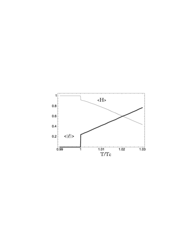
Figure 2: A cartoon sketching the gluon condensate $\langle H\rangle$ normalized to $\Lambda^{4}/e$ and the $\langle|\ell|\rangle$ (thick line) as function of temperature. We chose for illustration $a_{3}=0.3$, $a_{2}=1$, $\alpha=2$, $b_{1}=0.7$ and $T_{c}=1.2\Lambda$.

5 Conclusions

Our new theory is able to account for many features inherent to the Yang-Mills deconfining phase transition. We related two very distinct and relevant sectors of the theory: the hadronic sector (the glueballs), and some dimensionless fields ($\ell$) charged under the discrete group $Z_{N}$ understood as the center of the underlying $SU(N)$ Yang-Mills theory.

The gluon-condensate is, strictly speaking, not an order parameter for the deconfining Yang-Mills phase transition. However we have shown that the information encoded in the true order parameter $\ell$ is efficiently communicated to the gluon condensate. Since the exponential drop of the condensate just above the Yang-Mills critical temperature is a direct consequence of the behavior of the true order parameter at the transition we can consider this drop as a strong signal of deconfinement. This drop has already been used in various models for the Yang-Mills phase transition. We have also seen that the reduction in the gluon-condensate is associated to the increase of the Polyakov loop condensate $\ell$. The information about the order of the phase transition is also transferred to the behavior of the gluon condensate. Indeed, from Fig. 1 and Fig. 2 we deduce that the drop is continuous for the gluon condensate in the two color case, while is discontinuous for the three color theory. We now have a deeper understanding of the mechanism for transferring information from the Yang-Mills order parameter to the physical states. Other theoretical investigations also seem to support the present results [14].

It is worth mentioning that the Polyakov loop need not to be the only acceptable order parameter. For example using an abelian projection one can define a new (non local in the cromomagnetic variables) order parameter [15]. Our model can be, in principle, modified to be able to couple the hadronic states to any reasonable Yang-Mills order parameter.

Finally the present approach has also been extended to strongly interacting theories with fermions in the fundamental or adjoint representation of the gauge group. Within our framework we were then able to understand the relation between confinement and chiral symmetry breaking, and to make a number of predictions which can be tested via first principle lattice simulations [4].

It is now clear, that the critical behavior defined and governed by the order parameter can be studied via the singlet fields.

References

- [1] F. Sannino, Phys. Rev. D 66, 034013 (2002) [arXiv:hep-ph/0204174].
- [2] A. Mocsy, F. Sannino and K. Tuominen, Phys. Rev. Lett. 91, 092004 (2003) [arXiv:hep-ph/0301229].
- [3] A. Mocsy, F. Sannino and K. Tuominen, Induced universal properties and deconfinement, arXiv:hep-ph/0306069.
- [4] A. Mocsy, F. Sannino and K. Tuominen, Confinement versus chiral symmetry, arXiv:hep-ph/0308135.
- [5] G. Boyd, J. Engels, F. Karsch, E. Laermann, C. Legeland, M. Lutgemeier and B. Petersson, Nucl. Phys. B 469, 419 (1996) [arXiv:hep-lat/9602007].
- [6] M. Okamoto et al. [CP-PACS Collaboration], Phys. Rev. D 60, 094510 (1999) [arXiv:hep-lat/9905005].
- [7] B. Svetitsky and L. G. Yaffe, Nucl. Phys. B 210, 423 (1982). L. G. Yaffe and B. Svetitsky, Phys. Rev. D 26, 963 (1982). B. Svetitsky, Phys. Rept. 132, 1 (1986).
- [8] R. D. Pisarski, hep-ph/0112037; R.D. Pisarski, Phys. Rev. D62, 111501 (2000). A. Dumitru and R. D. Pisarski, Phys. Lett. B504, 282 (2001); hep-ph/0010083.
- [9] For a nice review on the effective Lagrangians related to the trace anomaly and a rather complete list of related references see: J. Schechter, arXiv:hep-ph/0112205. For more recent results on the subject see: F. Sannino and J. Schechter, Phys. Rev. D57, 170 (1998). S. D. Hsu, F. Sannino and J. Schechter, Phys. Lett. B 427, 300 (1998), hep-th/9801097. F. Sannino and J. Schechter, Phys. Rev. D60, 056004, (1999). For an application to high density QCD see R. Ouyed and F. Sannino, Phys. Lett. B 511 (2001) 66 [hep-ph/0103168].
- [10] F. Sannino and M. Shifman, Effective Lagrangians for orientifold theories, arXiv:hep-th/0309252.
- [11] A. Mocsy, F. Sannino and K. Tuominen, Confinement as Felt by Hadrons, in these proceedings.
- [12] P.H. Damgaard, Phys. Lett. B194 (1987) 107; J. Kiskis, Phys. Rev. D41 (1990) 3204; J. Fingberg, D.E. Miller, K. Redlich, J. Seixas, and M. Weber, Phys. Lett. B248 (1990) 347; J. Christensen and P.H. Damgaard, Nucl. Phys. B348 (1991) 226; P.H. Damgaard and M. Hasenbush, Phys. Lett. B331 (1994) 400: J. Kiskis and P. Vranas, Phys. Rev. D49 (1994) 528.
- [13] For a recent review and a rather complete list of references, see S. Hands, hep-lat/0109034.
- [14] P. N. Meisinger and M. C. Ogilvie, Phys. Rev. D 66, 105006 (2002) [arXiv:hep-ph/0206181].
- [15] A. D. Giacomo, arXiv:hep-lat/0204001.