Status of the computation of $f_{B_{s,d}}$, $\xi$ and $\hat{g}$

Abstract

Current status of the computation of the neutral $B$-meson mixing amplitudes, with particular attention to the heavy–light meson decay constants, is reviewed. The values for these quantities, as well as for the coupling of the pion to the lowest doublet of heavy–light mesons, are given.

Decay constants of heavy–light mesons enter in the most direct way the standard analyses of the CKM unitarity triangle [1, 2], namely through the frequencies of mixing in the neutral $B$-meson systems:

$$\Delta m_{d}=C_{B}m_{B_{d}}{f_{B_{d}}^{2}\hat{B}_{B_{d}}}A^{2}\lambda^{6}\left[(1-\bar{\rho})^{2}+\bar{\eta}^{2}\right]\,,$$ (1)

(2)

$${\Delta m_{d}\over\Delta m_{s}}={m_{B_{d}}\over m_{B_{s}}}\underbrace{f_{B_{d}}^{2}\hat{B}_{B_{d}}\over f_{B_{s}}^{2}\hat{B}_{B_{s}}}_{\displaystyle{1/\xi^{2}}}\lambda^{2}\left[(1-\bar{\rho})^{2}+\bar{\eta}^{2}\right]\,,$$ (3)

which, when combined with experimental values for the mass differences, constrain the vertex of the CKM triangle, through the circle in the $\bar{\rho}-\bar{\eta}$ plane. Pseudoscalar (and vector) meson decay constants, $f_{B_{d,s}}^{(\ast)}$, $f_{D_{u,s}}^{(\ast)}$, are also important in the studies of the corrections to the factorization approximation in non-leptonic $B$-decay modes. These constants are also important ingredients in the research of low energy physics effects coming from physics beyond Standard Model [3]. In what follows, I will focus on the computation of the pseudoscalar decay constants, although most of the discussion is equally applicable to the vector ones. I will briefly go through the novelties related to the bag-parameters $\hat{B}_{B_{d/s}}$, and close this short review by discussing the value of the phenomenologically important coupling of the pion to the lowest–lying doublet of heavy–light mesons.

1 Strategies and difficulties to compute
the decay constants

The decay constant $f_{H}$ of the heavy–light pseudoscalar meson $H$ is defined through

$$\langle 0|\bar{Q}\gamma_{\mu}\gamma_{5}q|H(p)\rangle=ip_{\mu}f_{H}\,,$$ (4)

where $Q$ is either $c$- or $b$-quark, and $q$ is $s$- or $u/d$-quark.  Although the matrix element (4) is the simplest one, the fact that one quark is heavy and the other is light makes its computation extremely difficult (in spite of the simplifications stemming from the heavy quark and chiral symmetries).

In various quark models the decay constant is either a parameter of the model, or its value depends crucially on the specific choice of the model’s parameters. This situation is clearly unacceptable as we seek a “model-independent” estimate (an ab initio determination), solely relying on the underlying theory, on QCD. A step in this direction was made by employing the duality sum rules, both in QCD and in heavy quark effective theory (HQET).  The non-perturbative contributions in this approach are parametrized by the power corrections, the coefficients of which are the vacuum condensates. Apart from the chiral condensate, the essential non-perturbative input in evaluating $f_{B}$ comes from the gluon and the mixed quark-gluon condensates. Those two are either not well defined or their values are poorly known. For example, the gluon condensate, as estimated from the comparison of the sum rules with the corresponding experimental information on the $\rho^{(n)}$ resonances [5] and charmonium resonances [6], differ by a factor of roughly $8$:

$$\left<{\alpha_{s}\over\pi}G_{\mu\nu}^{2}\right>=\biggl{.}(0.074\pm 0.023)\ {\rm GeV}^{4}\biggr{|}_{``\rho"}\!\!,\biggl{.}(0.009\pm 0.007)\ {\rm GeV}^{4}\biggr{|}_{``\psi"}\!\!.$$

Besides, it is often unclear where the onset of the quark–hadron duality in the sum rule takes place (parametrized by the threshold parameter $s_{0}$). In short, the benefit of the method is that it made a step towards the first principle QCD calculations of the hadronic quantities; the drawback is the existence of too many parameters whose values are loosely constrained, thus prohibiting the precision determination of the hadronic quantities, and of $f_{B}$ in particular.

Lattice QCD is the closest to our ultimate goal, first-principle QCD calculation of the matrix element (4). Although the calculations are based on the numerical simulations of the QCD vacuum fluctuations, the great bonus is that the only parameters appearing in the computations are those that appear in the QCD Lagrangian, namely the bare strong coupling and quark masses. A strategy to compute $f_{B}$ on a 4-dimensional lattice ($L^{3}\times T$) is very simple and can be summarized in $4$ steps:

• Generate an SU(3) gauge field configuration ${\cal U}$ (by using the Monte Carlo technique);

• For each time slice, $t\in[0,T)$, in the background field produced in 1, calculate the correlation function,

  $$\sum_{\vec{x}}\langle 0|\overbrace{\bar{Q}(x)\gamma_{0}\gamma_{5}q(x)}^{\displaystyle{A_{0}(x)}}A_{0}^{\dagger}(0)|0\rangle.$$ (5)

• Repeat steps 1 and 2, a number $N_{\rm conf.}$ of times, $N_{\rm conf.}$ refering to the number of independent gauge field configurations. From the average over the statistical sample, extract $f_{H}$ as

  $$\langle\sum_{\vec{x}}A_{0}(x)A_{0}^{\dagger}(0)\rangle_{\cal U} \stackrel{{\scriptstyle t\gg 0}}{{=}} {|\langle 0|\bar{Q}\gamma_{{}_{0}}\gamma_{{}_{5}}q|H\rangle|^{2}\over 2m_{H}}e^{-m_{H}t}\,+\,\dots$$ (6)

  $$= {1\over 2}{f_{H}^{2}}m_{H}e^{-m_{H}t}\,+\,\dots\;,$$

  where the (euclidean) time is large enough for the higher (heavier) excited states to be indeed suppressed w.r.t. the lowest lying one;

• Repeat 2 and 3 for several different light and heavy quark masses, $m_{q}$ and $m_{Q}$ respectively.

This simple procedure is very demanding in practice: to avoid large lattice artefacts, while working with reasonably light quarks, the size of the lattice box ($L$) must be very large. Simultaneously, and to resolve the propagation of the heavy quark, a very small lattice spacing (“$a$”) is needed. Compared with the physical quark masses, the currently available computers allow us to work with

$$m_{c}\leq m_{Q}<m_{b}\,,\ {\rm and}\quad m_{u/d}<m_{q}\leq m_{s}\;.$$ (7)

In other words, we can directly compute only the $f_{D_{s}}$ decay constant.

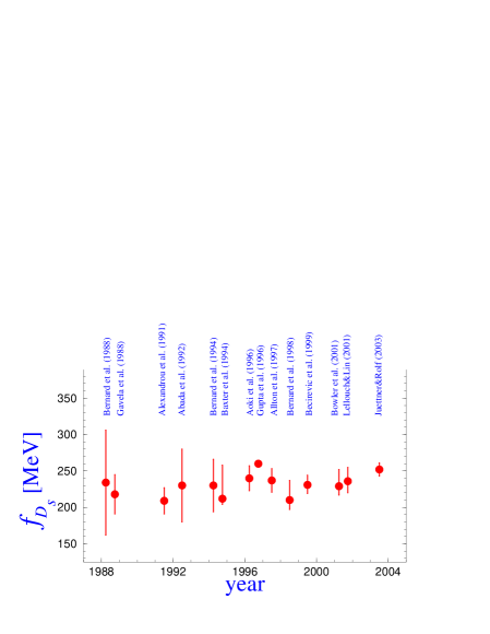
Figure 1: Evolution of the lattice estimates of $f_{D_{s}}$, as obtained by various lattice groups. List of papers corresponding to the above results, organized chronologically, can be found in refs. [7, 8]. The last result, from ref. [9], is the final lattice value obtained in the quenched approximation.

In fig. 1 we present the evolution of the results obtained from the lattice QCD simulations over the past 15 years. All results are obtained in the quenched approximation. The last value is actually the final quenched lattice estimate for this quantity. It is obtained after implementing all the important elements of theoretical progress made in the 90’s, namely: (i) the quark action and the axial current are improved, providing a better scaling to the continuum limit; (ii) the local axial current defined on the lattice is matched to its continuum counterpart non-perturbatively; (iii) the simulations are made at several (four) small lattice spacings “$a$”, which allows for a smooth extrapolation to the continuum limit ($a\to 0$). The final result of ref. [9] is

$$f_{D_{s}}=252\pm 9\ {\rm MeV}.$$ (8)

The fact that the $b$-quark cannot be resolved on the available lattices opened three options:

• Compute $f_{H}$ for the accessible $m_{Q}$ and then from the fit of $\Phi(m_{Q})=C(m_{Q})f_{H}\sqrt{m_{H}}$, in $1/m_{H}$, extrapolate to the $B$-meson mass. $\Phi(m_{Q})$ is the quantity that scales with the inverse quark(meson) mass as a constant. The sizable $1/m_{H}$ corrections are determined from the lattice data. The resulting values, however, have large errors, mainly due to uncertainty of whether or not one includes the terms of ${\cal O}(1/m_{H}^{n\geq 2})$ in the extrapolation. Besides, the larger quark masses may induce large lattice cut-off artefacts that are hard to quantify.

• Difficulties in controlling the systematic errors of the strategy (a) incited many groups to attempt treating the heavy quark in an effective theory. Computation of the matrix element (4) in the static limit of HQET [10] turned out to be very difficult, mainly because of the very poor signal [11]. That problem (of the poor signal) was circumvented by including the ${\cal O}(1/m_{Q})$ corrections in both the Lagrangian and in the operator (axial current) by discretizing the NRQCD [12]. In spite of its benefits (working with large quark masses) this method cannot be used for the precision computation since, on the lattice, the $1/m_{Q}$ terms become ${\cal O}[1/(am_{Q})]$, where $``a"$ is the small lattice spacing. In other words, the continuum limit does not exist. Besides, in both approaches (HQET and NRQCD) the non-perturbative renormalization of the axial current was not feasible. The third effective approach has been developed by the Fermilab group [13]. It consists of pushing the propagating heavy quark, $Q$, over the lattice cut-off and then expanding in powers of $1/m_{Q}$ [not $1/(am_{Q})$]. The key in that procedure is to match the relativistic with non-relativistic energy-momentum dispersion relations, where the mismatch is accounted in distinguishing the masses that appear in the non-relativistic expansion as $M_{``static"}$, $M_{``kinetic"}$, and so on. That matching is typically made non-perturbatively while the renormalization is made only perturbatively. 

• Combine the value of $\Phi(\mu)$ obtained in the static limit ($1/m_{Q}=0$), with the decay constants computed with the directly accessible heavy–light mesons, and interpolate to $1/m_{b}$. The main obstacles in following this strategy, as mentioned above, are the poor statistical quality of the static correlation functions and the missing non-perturbative evaluation of the renormalization constant.

The overall agreement among results for $f_{B_{s}}$, as obtained by using various strategies, was quite impressive. However, none of the approaches was fully satisfactory to provide a precision measurement (even within the quenched approximation). This is why the errors remained essentially unchanged over the last 7 years, as can be seen in fig. 2, where we plot the evolution of the world average of the quenched lattice estimates of $f_{B_{s}}$ [15].

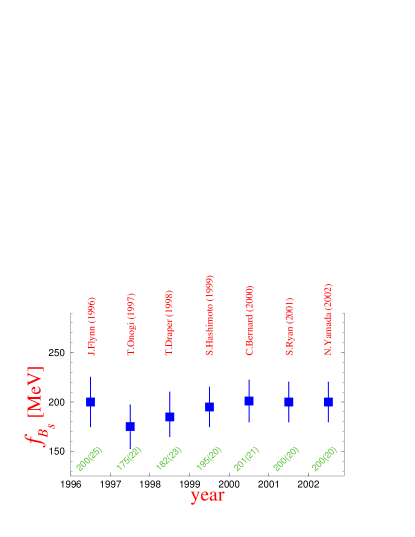
Figure 2: Evolution of the world average of the (quenched) lattice estimates of $f_{B_{s}}$, reported at the annual “Lattice” meetings [15]. In the average enter the results obtained by all the strategies to treat the heavy quark on the lattice that are discussed in the text.

2 New ways to get $f_{B_{s}}$ (quenched)

The two results, reported this year, actually supersede all the previous quenched calculations.

2.1 Method of finite volumes

To simulate the $b$-quark directly on the lattice, one can actually set a very small lattice spacing, but then the physical volume becomes too small to accommodate the propagation of the light quark. To get around this problem, the “Tor Vergata” group [16] proceed as follows: (i) in a small box of side $L=L_{0}$, they compute $f_{H}(L_{0})$; (ii) they double the side of the box, at fixed lattice spacing $a$, recompute $f_{H}(2L_{0})$, and take the ratio, $\Sigma_{2}(a)=f_{H}(2L_{0})/f_{H}(L_{0})$; (iii) step (ii) is then repeated $n$ times until $\Sigma_{2n}(a)\to 1$; (iv) the whole procedure is redone for several values of the lattice spacing $a$, allowing the smooth continuum extrapolation, $\Sigma_{2n}(a)\to\Sigma_{2n}(0)\equiv\sigma_{2n}$. Throughout the calculation, they set $T=2L$, and extract the decay constant precisely at $T/2$.

The actual calculation with this clever procedure was recently completed in ref. [17]. Let us first focus on $f_{D_{s}}$. In the first step, they work with $L_{0}=0.4$ fm, so that at $t=L_{0}$ they certainly cannot extract $f_{D_{s}}(L_{0})$, but rather

$$f_{D_{s}}^{\rm eff.}(L_{0})=f_{D_{s}}(L_{0})\left[1+\sum_{n}\sqrt{m_{D_{s}^{(n)}}f_{D_{s}^{(n)}}^{2}\over m_{D_{s}}f_{D_{s}}^{2}}e^{-(m_{D_{s}^{(n)}}-m_{D_{s}})L_{0}}\right]\,,$$ (9)

where the sum runs over all excitations that are not heavy enough to be exponentially suppressed at (small) $L_{0}$. After doubling the size, $L_{0}\to 2L_{0}$, the exponential suppression will be more efficient, so that after $2$ or $3$ steps all excitations will die out. After performing the continuum extrapolation in each step, they obtain

$$f_{D_{s}}^{\rm eff.}(L_{0})=644\pm 3\ {\rm MeV}, \sigma_{2}={f_{D_{s}}^{\rm eff.}(2L_{0})\over f_{D_{s}}^{\rm eff.}(L_{0})}=0.414(3),$$ (12)

$$\sigma_{4}={f_{D_{s}}^{\rm eff.}(4L_{0})\over f_{D_{s}}^{\rm eff.}(2L_{0})}=0.90(2),$$

$$\Longrightarrow\ f_{D_{s}}=f_{D_{s}}^{\rm eff.}(L_{0})\sigma_{2}\sigma_{4}=240(5)(5)\ {\rm MeV}\,,$$

thus in good agreement with the value obtained in ref. [9]. The main reason why $\sigma_{2}$ is so different from $1$ seems to be the presence of the non-decoupled excited states. This can be seen from what the authors of ref. [17] present: they show that $\Sigma_{2n}(a)$ depends only weakly on both the heavy and light quark masses, and they verify only a tiny dependence on the lattice spacing.

When working with the $B_{s}$-meson, $f_{B_{s}}^{\rm eff.}(L_{0})$ can be computed directly, but doubling the side of the box to compute $\sigma_{2n}$ becomes unfeasible. Instead, one can afford to compute $\sigma_{2n}(m_{Q})$, for $m_{c}\lesssim m_{Q}\lesssim m_{b}/2$, and then reach $\sigma_{2n}(m_{b})$, through an extrapolation. For that purpose they assume the heavy quark expansion in the finite box, so that

$$\sigma_{2n}(m_{Q})=\alpha_{2n}+\beta_{2n}/m_{Q}\,,$$ (13)

where the constant $\beta$ naively scales as $1/(2^{n-1}L_{0})$. Their data indeed verify eq. (13), leading to

$$f_{B_{s}}^{\rm eff.}(L_{0})=475\pm 2\ {\rm MeV}, \sigma_{2}(m_{b})=0.417(3),$$ (16)

$$\sigma_{4}(m_{b})=0.97(3),$$

$$\Longrightarrow\ f_{B_{s}}=f_{B_{s}}^{\rm eff.}(L_{0})\sigma_{2}(m_{b})\sigma_{4}(m_{b})=192(6)(4)\ {\rm MeV}\,.$$

The second error indicates the combined systematic uncertainty due to renormalization constants and to the continuum extrapolations.

2.2 Combining with the static $f_{B_{s}}$

As we mentioned before, the value of the decay constant in the static limit was plagued by two main difficulties: 1. the renormalization of the axial current in HQET on the lattice; 2. bad signal-to-noise ratio. Both problems have been solved recently.

By a judicious choice of the renormalization condition, the authors of ref. [18] provided a solution to the first problem (see around eq.(2.15) of that paper). They devised the method of subtracting the power-divergent residual mass counterterm non-perturbatively, which then allowed them to apply the standard non-perturbative renormalization procedure in the Schrödinger functional scheme [19].

The solution to the second problem came recently too [20]. In the static limit, eq. (5) becomes

$$C^{\rm cont.}(t)=\langle{\rm Tr}\left({1+\gamma_{0}\over 2}{\cal S}_{q}(\vec{0},t){\cal P}{\rm e}^{ig\int_{0}^{t}d\tau A_{0}(\vec{0},\tau)}\right)\rangle$$ (17)

$$\rightarrow C^{\rm latt.}(t)=\langle{\rm Tr}\left({1+\gamma_{0}\over 2}{\cal S}_{q}(\vec{0},t)\prod_{\tau=1}^{t-1}U_{0}(\tau)\right)\rangle\ ,$$ (18)

where ${\cal S}_{q}(\vec{0},t)$ is the light quark propagator at $\vec{x}=0$, while the Wilson line on the lattice is simply the time-ordered product of link variables. Empirically, the statistical quality of $C^{\rm latt.}(t)$ becomes much better if some kind of “fattening” of the link variable is made: $U_{0}(\tau)\to U_{0}^{\rm fat}(\tau)$. 

After extrapolating to the continuum limit and converting the static HQET result to QCD, from ref. [20] we learn that,

$$f_{B_{s}}^{\rm stat}=225\pm 16\ {\rm MeV}.$$ (19)

That result has then been combined with those that are accessible directly, with the propagating heavy quark of mass $(am_{Q})\lesssim 0.65$ (in lattice units) as to avoid larger discretization errors. After extrapolating to the continuum at each of the simulated heavy quarks, they show a very smooth linear behaviour of the combined set of data. Their preliminary result, presented in ref. [22], is:

$$f_{B_{s}}=206\pm 10\ {\rm MeV}.$$ (20)

The bonus of that result is obviously a much better precision, since the extrapolation to $b$-quark is now replaced by the interpolation. Notice however that the slope (i.e. $1/m_{Q}$-dependence) of $\Phi_{Q}\equiv Cf_{H_{s}}\sqrt{m_{H_{s}}}$, quoted in ref. [22], is completely compatible with the previous calculations in which the strategy with propagating heavy quark was used at a fixed value of the lattice spacing.

2.3 Status and perspectives of quenched $f_{D_{s}}$ and $f_{B_{s}}$

After $15$ years of computing the heavy–light decay constants on the lattice, in the quenched approximation, we are finally in a position to quote the precise values. From the results discussed in this section, I conclude

$$f_{D_{s}}^{N_{\rm f}=0}=245\pm 6\ {\rm MeV}\,,\quad f_{B_{s}}^{N_{\rm f}=0}=194\pm 6\ {\rm MeV}\,.$$ (21)

It should be stressed that these values are obtained by fixing the lattice spacing to $r_{0}=0.5$ fm, which, however, is an assumption. Using other quantities, such as $f_{K}$, $m_{K^{\ast}}$, leads to different values, which amount to a systematic error of about $5\%$. The above results are obtained by working with fine-grained lattices, by implementing the non-perturbative renormalization and after a smooth extrapolation to the continuum limit. Alpha group plans to attempt a computation of the $1/m_{b}$ corrections to the $f_{B_{s}}^{\rm stat}$, to check whether these are enough to feed the linear dependence that they observed after having combined the static and the results obtained with relativistic (propagating) heavy quarks [22].

The most challenging issue that remains to be studied and understood is to assess the error induced by the quenched approximation. The knowledge gained about that systematics is what we discuss next.

3 Unquenching $f_{D_{s}}$ and $f_{B_{s}}$

To unquench the lattice results means that one has to include the effects of dynamical quarks (those popping up through loops in the background gauge field). To incorporate the light dynamical quarks is, in principle, possible, but very costly in practice. The most tested and widely used robust algorithm, Hybrid Monte Carlo (HMC) [23], allows one to include two light degenerate quarks of the mass close to the strange quark (please see [24]). Getting to the quarks lighter than half of the strange quark mass is nowadays impossible, if we use the standard Wilson quark action and keep the finite volume effects under control. To get over that limit, as well as to include the third (strange) dynamical quark, a substantial progress in algorithm building is badly needed. An important step in that direction has been made in ref. [25].

Up to now, the partially (un)quenched computations are made by using the Wilson quark action for the light and one of the effective approaches to treat the heavy quark.

By confronting the results of quenched and unquenched studies (with $N_{\rm f}=2$ degenerate sea quarks) obtained by using the NRQCD treatment of the heavy quark on the lattices with $a^{-1}\approx 2$ GeV [26, 27, 28], the following effect of the dynamical quarks can be deduced :

$${\rm CP-PACS}\!\!\!\!\!\! : {f_{B_{s}}^{N_{\rm f}=2}\over f_{B_{s}}^{N_{\rm f}=0}}=1.10(5)\,,$$ (22)

$${\rm JLQCD}\!\!\!\!\!\! : {f_{B_{s}}^{N_{\rm f}=2}\over f_{B_{s}}^{N_{\rm f}=0}}\simeq 1.13(5)\,.$$ (23)

With the Fermilab treatment of the heavy quark, instead, one has [29, 30]: 

$${\rm CP-PACS}\!\!\!\!\!\! : {f_{B_{s}}^{N_{\rm f}=2}\over f_{B_{s}}^{N_{\rm f}=0}}=1.14(5)\,,\quad{f_{D_{s}}^{N_{\rm f}=2}\over f_{D_{s}}^{N_{\rm f}=0}}=1.07(5)\,,$$ (24)

$${\rm MILC}\!\!\!\!\!\! : {f_{B_{s}}^{N_{\rm f}=2}\over f_{B_{s}}^{N_{\rm f}=0}}\simeq 1.09(5)\,,\quad{f_{D_{s}}^{N_{\rm f}=2}\over f_{D_{s}}^{N_{\rm f}=0}}\simeq 1.08(5)\,.$$ (25)

The average of the above results, combined with the values given in eq. (21), leads to

$${f_{B_{s}}^{N_{\rm f}=2}\over f_{B_{s}}^{N_{\rm f}=0}}=1.12(5)\,\Rightarrow\,f_{B_{s}}^{N_{\rm f}=2}=217\pm 12\ {\rm MeV},$$ (26)

$${f_{D_{s}}^{N_{\rm f}=2}\over f_{D_{s}}^{N_{\rm f}=0}}=1.08(5)\,\Rightarrow\,f_{D_{s}}^{N_{\rm f}=2}=265\pm 14\ {\rm MeV}.$$ (27)

Unaccounted for is $\sim 5\%$ of systematic uncertainty, which we should keep in mind, due to the scale setting when converting from the lattice to the physical units. A detailed study of that uncertainty in the unquenched ($N_{\rm f}=2$) simulations has not been made so far.

Finally, we are interested in the situation in which $N_{\rm f}=2+1$, where the extra flavour would correspond to the strange sea quark. With Wilson fermions such a study is extremely expensive, although the algorithms to do such simulations already exist [31]. Instead, a study with the so-called staggered light quarks has been made [32]. Although the method is relatively cheap to implement, one of the unsatisfactory features can be formulated as follows. With the staggered action, each dynamical quark flavour on the lattice comes in four “tastes” (copies), and it is unclear how one can relate such Dirac determinant $\Delta_{\rm staggered}$, to the desired one. A current practice of taking $+\left(\Delta_{\rm staggered}\right)^{1/4}$ induces non-localities that are potentially problematic, and the whole formulation may not correspond to QCD. The proponents of the method will hopefully study this issue more carefully. Having that off my chest, I can now compare the quenched and unquenched results of ref. [32], in which the NRQCD treatment of the heavy quark has been used, to quote

$$\left(f_{B_{s}}^{N_{\rm f}=2+1}/f_{B_{s}}^{N_{\rm f}=0}\right)\approx 1.15\,,$$ (28)

i.e. fully consistent with the result in eq. (26).

In conclusion, the current values of the pseudoscalar decay constants, with the light quark $s$, are:

4 $f_{B_{s}}/f_{B_{u/d}}$ and $f_{D_{s}}/f_{D_{u/d}}$

So far we discussed the case with the strange light quark in the heavy–light meson. In particle physics phenomenology, however, more needed is the information about $f_{B_{u/d}}$, $f_{D_{u/d}}$, and about the SU(3) breaking ratios, $f_{B_{s}}/f_{B_{u/d}}$ and $f_{D_{s}}/f_{D_{u/d}}$. The best known example of how important is the knowledge of these quantities is the one given in eq. (1).

As we already pointed out in the previous sections, the physical $m_{u/d}$ is too small to be simulated directly on the lattice. Currently feasible are the light quarks whose mass, with respect to the physical strange quark mass ($r=m_{q}/m_{s}^{\rm phys.}$), lie between

$$1/2\ \lesssim\ r\ \lesssim 2\,,$$ (32)

implying the necessity for quite a long extrapolation to the physically relevant limit, $r\to r_{u/d}=0.04$ [33]. This is where the staggered quark action has a great advantage over the standard (Wilson) one: due to the explicit chirality, with staggered quarks one can reach quarks as light as $r\approx 1/4$ [32], implying a better control over the extrapolation to $r_{u/d}$.

Within the accessible range of the light quark masses (32), the results of both quenched and unquenched simulations (with $N_{\rm f}=2$) suggest a pronounced linear dependence on the light quark mass,

$${f_{B_{s}}\over f_{B_{q}}}\ =\ 1\ +\ X_{b}\cdot(1-r)\,,$$ (33)

with little or no room for a term $\propto r^{2}$. For the quenched value of the slope $X_{b}$, I will take the one quoted in ref. [17], namely $X_{b}^{N_{\rm f}=0}=0.13(2)(1)$. To get the unquenched slope, we first compile the available results for the SU(3) breaking ratio as computed with $N_{\rm f}=2$, divided by its quenched value, where both results are being obtained from an extrapolation of the form (33).

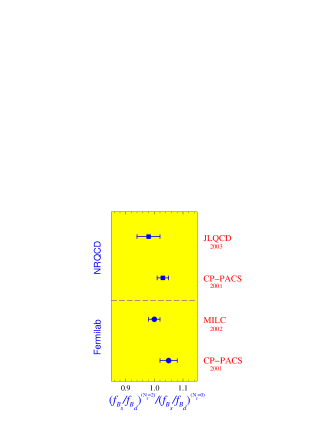
Figure 3: Ratio of the slopes which appear in eq. (33) in light quark mass, as obtained from the quenched and unquenched simulations, by using the NRQCD and the Fermilab treatment of the $b$-quark. From up to down, the results correspond to refs. [27, 28],[26], [30] and [29].

Those results are plotted in fig. 3. The average is

$${\;(f_{B_{s}}/f_{B_{d}})^{N_{\rm f}=2}\over(f_{B_{s}}/f_{B_{d}})^{N_{\rm f}=0}}=1.02\pm 0.03\,,$$ (34)

or, the SU(3) breaking ratio is only slightly sensitive to the switch from $N_{\rm f}=0\to 2$, for the light quark mass in the range indicated in eq. (32). Notice also that a preliminary study with staggered fermions indicates that this feature persists even after going to ${N_{\rm f}=2+1}$. From the above discussion we can now easily extract the slope:

$$X_{b}^{N_{\rm f}=2}=0.15(4)\,.$$ (35)

A common practice “to use a ruler” and extrapolate the observed behaviour to the physical $r\to r_{u/d}$ is, however, dangerous because one is getting deeply into the region dominated by the spontaneous chiral symmetry breaking effects, so that the observed linear behaviour of the decay constants w.r.t. the change of the light quark mass may be significantly modified. That problem was first pointed out in ref. [35], and recently in [36]. It is therefore of paramount importance to do the computation with the light quark as light as possible, and check for the deviation from the form (33). In doing so, the finite volume effects should, of course, be kept under control. That is where the $\epsilon$-expansion should be applied in the way similar to what has been done recently in ref. [37].  Since such an unquenched study is not around the corner, we may rely on the chiral perturbation theory (ChPT) to guide the (chiral) extrapolations. By using the Lagrangian in which the ChPT is combined with the static limit of HQET, the chiral logarithmic corrections to the SU(3) breaking ratio of the decay constants has been computed in [38]

$$R_{B_{s/d}}^{\rm ChPT}\equiv{f_{B_{s}}\sqrt{m_{B_{s}}}\over f_{B_{d}}\sqrt{m_{B_{d}}}}=1\!\!\! + \!\!\!{1+3{\hat{g}}^{2}\over 4(4\pi f)^{2}}\left(3m_{\pi}^{2}\log{m_{\pi}^{2}\over\Lambda_{\chi}}\right.$$ (37)

$$\left.-2m_{K}^{2}\log{m_{K}^{2}\over\Lambda_{\chi}}-m_{\eta}^{2}\log{m_{\eta}^{2}\over\Lambda_{\chi}}\right)+{8K(\Lambda_{\chi})\over f^{2}}(m_{K}^{2}-m_{\pi}^{2})\,,$$

where $K$ stands for the unknown low energy constant. $R_{B_{s/d}}^{\rm ChPT}$ is independent of the chiral symmetry breaking scale $\Lambda_{\chi}\simeq 1$ GeV. This formula can be cast into the form ready for extrapolation by using the GMOR and Gell-Mann–Okubo formulae,

$$m_{\pi}^{2}=2B_{0}m_{s}r\,,\quad m_{K}^{2}=2B_{0}m_{s}{r+1\over 2}\,,\quad m_{\eta}^{2}=2B_{0}m_{s}{r+2\over 3}\,.$$

After noticing that $2B_{0}m_{s}=2m_{K}^{2}-m_{\pi}^{2}=(684\ {\rm MeV})^{2}$, eq. (37) can be written in terms of $r$, which we will then call $R_{B}^{\rm ChPT}(r)$. Notice that the last term is $\propto(1-r)$, much like in eq. (33) in which the slope was obtained from the fit to the lattice data, and which we will refer to [eq. (33), that is] as $R_{B}^{\rm latt}(r)$. The main trouble actually lies in the fact that the chiral logarithms are multiplied by the large coefficient $(1+3g^{2})\approx 1.8$,  so that the application of the form $R_{B}^{\rm ChPT}(r)$ to extrapolate to $r_{u/d}$ results in a large shift, compared to what we obtain from the naive extrapolation, i.e. from the result of the application of $R_{B}^{\rm latt}(r_{u/d})$. Since we do not directly observe the chiral logarithms on the lattice, the formula $R_{B}^{\rm ChPT}(r)$ can be used only below the region of the quark masses covered by our lattice simulations, namely for $r<r_{M}\simeq 0.5$. It can also be argued that $R_{B}^{\rm ChPT}(r)$ is not appropriate for the ‘pions’ as heavy as $m_{``\pi"}=0.48$ GeV ($\Leftrightarrow\ r_{M}=0.5$), and the form $R_{B}^{\rm latt}(r)$ can be extrapolated to lower $r_{M}$, before including the ChPT formula in the extrapolation. Clearly, the point $r_{M}$, at which the smooth matching can be made,

$$R_{B_{s/q}}(r) = \vartheta(r-r_{M})R_{B_{s/q}}^{\rm latt}(r)$$ (40)

$$+\vartheta(r_{M}-r)\biggl{[}R_{B_{s/q}}^{\rm ChPT}(r)-\left(R_{B_{s/q}}^{\rm ChPT}(r_{M})-R_{B_{s/q}}^{\rm latt}(r_{M})\right)\biggr{.}$$

$$\biggl{.}-\left(\left.{\partial R_{B_{s/q}}^{\rm ChPT}/\partial r}\right|_{r=r_{M}}+X_{b}\right)(r-r_{M})\biggr{]},$$

will result in different shifts. By taking $r_{M}=0.75$, a pure SU(3) breaking effect, $f_{B_{s}}/f_{B_{d}}-1$, gets enhanced by $100\%$ [36]. If, instead, we take $r_{M}=0.25$, the shift is still $+30\%$. This is illustrated in fig. 4. An equivalent way to see that feature has been discussed in ref. [39], where the chiral loop integrals are computed by introducing the hard cut-off. The uncertainty on the value of the cut-off scale corresponds precisely to the uncertainty of the position in $r_{M}$ discussed above.

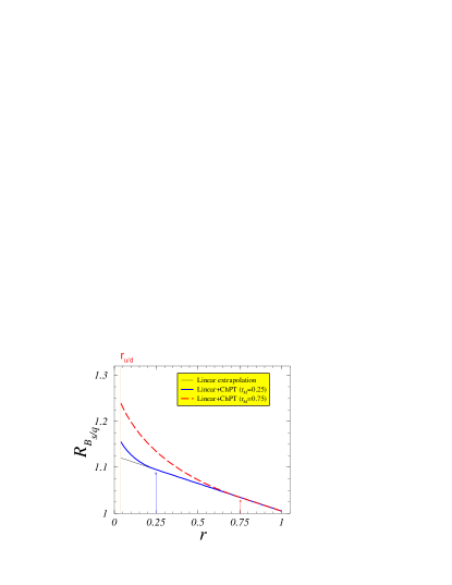
Figure 4: Illustration of the shift induced by the chiral logarithms in the extrapolation from the light quark masses accessed from the lattice, $r\in(0.5,1]$, to the physical point, $r_{u/d}=0.04$. The sensitivity of the resulting $f_{B_{s}}/f_{B_{d}}$ on the choice of the matching point $r_{M}$ [see eq. (40)] is also shown. The phenomenon is illustrated by using $X_{b}=0.12(2)(3)$, and $g=0.5$.

To get around that uncertainty, before we are able to work with the light quarks sufficiently close to the chiral limit on the lattice, in ref. [40] it was proposed to study the double ratio

$$R(r)={R_{B_{s/q}}(r)\over f_{K_{sq}}/f_{\pi_{qq}}}\,.$$ (41)

There are two reasons why this is advantageous:

• The coefficients multiplying the chiral logarithms in

  $$R^{\rm ChPT}_{\pi_{u/d}}\equiv{f_{K}\over f_{\pi}}=1\!\!\!\!\! + \!\!\!\!\!{1\over 4(4\pi f)^{2}}\left[5m_{\pi}^{2}\log{m_{\pi}^{2}\over\Lambda_{\chi}}-2m_{K}^{2}\log{m_{K}^{2}\over\Lambda_{\chi}}\right.$$ (43)

  $$\left.-3m_{\eta}^{2}\log{m_{\eta}^{2}\over\Lambda_{\chi}}\right]+{8L_{5}(\Lambda_{\chi})\over f^{2}}(m_{K}^{2}-m_{\pi}^{2})\,,$$

  have the same sign and are almost of the same size as those appearing in eq. (37).  Therefore, in the ratio, the logarithms will cancel to a large extent and the form

  $$R(r)\ =\ A\ +\ B\cdot(1-r)\,$$ (44)

  can be used in extrapolations, with a very small error due to the uncancelled logarithms. Using an equation similar to (40), but for $R(r_{u/d})$, we notice a weak (negligible) sensitivity on the choice of $r_{M}$, because the large logarithms are cancelled.

• The physical result is obtained after multiplying $R(r_{u/d})$ by $f_{K}/f_{\pi}$, which is known from experiment, namely $f_{K}/f_{\pi}=1.22(1)$ [41].

Concerning $f_{K}/f_{\pi}$, it is important to stress that, compared with the experimental value, the quenched lattice estimates obtained after extrapolating linearly,

$$R^{\rm latt}_{\pi}\ =\ 1\ +\ X_{q}\cdot(1-r)\,,$$ (45)

always lead to a small value. For example, from the SPQcdR data [42], in the continuum limit, I get $X_{q}^{N_{\rm f}=0}=0.12(2)$, which then amounts to, $f_{K}/f_{\pi}-1=0.11(2)$, i.e. $50\%$ smaller than the experimental value. The folkloric explanation for this “spectacular failure” was/is the use of the quenched approximation. JLQCD collaboration recently showed that this is, however, not totally true. From their precision quenched and unquenched ($N_{\rm f}=2$) computation, the results of which are reported in ref. [43], I read off 

$$X_{q}^{N_{\rm f}=0}=0.125(7),\quad X_{q}^{N_{\rm f}=2}=0.154\left({}^{+16}_{-12}\right).$$ (46)

The missing piece that would help getting to $(f_{K}/f_{\pi})^{\rm exp.}$ is likely to be the one due to the chiral logarithms. This situation is precisely the opposite to the one that incited the ChPT practitioners to make the consistent NLO calculations, because the chiral logs alone give $f_{K}/f_{\pi}\simeq 1.14$, whereas at NLO the low energy constant $L_{5}$ [see eq.(43)], is fixed so as to reproduce $(f_{K}/f_{\pi})^{\rm exp.}$ [44] . On the lattice, instead, we see the explicit linear quark mass dependence but there is still no clear evidence for the presence of the chiral logs (most probably because we are not working with sufficiently light quarks). To get the lattice estimate of $f_{K}/f_{\pi}$, we then face the same problem as before: chiral logs are large and the results of extrapolation by using an expression similar to eq. (40) would be strongly dependent on the choice of the matching point $r_{M}$.

The double ratio (41) avoids all those headaches, and can be computed on the lattice directly. By combining $X_{q}=0.154\left({}^{+16}_{-12}\right)$, with $X_{b}=0.15(4)$, I get

$${f_{B_{s}}\over f_{B_{d}}} = {f_{K}^{\rm exp}\over f_{\pi}^{\rm exp}}\left[{1\ +\ X_{b}\cdot r_{u/d}\over 1\ +\ X_{q}\cdot r_{u/d}}+\sqrt{m_{B_{d}}\over m_{B_{s}}}\times{\rm``chi-logs"}_{\hat{g}}\right]$$ (47)

$$= 1.21\pm 0.05\pm 0.01\,,$$ (49)

where the last error is due to the variation of the coupling $\hat{g}=0.52(7)(7)$. A similar proposal, to consider $\sqrt{m_{B}}f_{B}/f_{\pi}$, has been made in ref. [30]. However, one has to assume that the terms of ${\cal O}(1/m_{b})$, which are known to be large, do not induce any extra chiral log dependence. Large ${\cal O}(1/m_{b})$ correction cancel in the $f_{B_{s}}/f_{B}$ ratio.

A completely analogous procedure to the one sketched above applies to the charm sector. I will use $X_{c}=0.11(4)$, which is obtained from $X_{c}^{N_{\rm f}=0}=0.09(1)(1)$ [17], and the observation made in refs. [29, 30], namely $(f_{D_{s}}/f_{D})^{N_{\rm f}=2}/(f_{D_{s}}/f_{D})^{N_{\rm f}=0}=1.02(3)$. Together with the experimentally measured $\hat{g}_{c}=0.61(6)$, and from the formula analogous to eq. (47), I arrive at ${f_{D_{s}}/f_{D}}=1.22(4)$.

In summary,

or, within the error bars, $f_{B_{s}}/f_{B}\approx f_{D_{s}}/f_{D}\approx f_{K}/f_{\pi}$.

5 $B_{q}^{0}-\overline{B^{0}_{q}}$ mixing and $\xi$

The bag parameter that parameterizes the $B_{q}^{0}-\overline{B^{0}_{q}}$ mixing amplitude is defined by

$$\langle\bar{B}^{0}_{q}|\bar{b}^{i}\gamma_{\mu}(1-\gamma_{5})q^{i}\,\bar{b}^{j}\gamma_{\mu}(1-\gamma_{5})q^{j}|B^{0}_{q}\rangle={8\over 3}\,m_{B_{q}}^{2}f_{B_{q}}^{2}\hat{B}_{B_{q}}\ ,$$ (53)

i.e. normalized to the vacuum saturation approximation ($B_{VSA}=1$). This amplitude is very difficult to calculate by QCD sum rules because: (i) the calculation of the NLO corrections to the perturbative part of the spectral function, as well as to the Wilson coefficients multiplying the condensate contributions, is quite involved; (ii) the stability of the sum rule under the variation of the threshold and the Borel parameters is very hard to achieve. Some progress concerning the first part of the problem was made recently in ref. [46]. So far, the lattice QCD studies of the matrix element (53) are made by using the Wilson quark action. The unpleasant feature of the Wilson quarks is the lack of explicit chirality, which induces complications in renormalization, namely it allows the operator in eq. (53) to mix with other parity-even, $\Delta B=2$, dimension-six operators. The extra mixing is the lattice artefact and should be subtracted, preferably non-perturbatively. To a discussion provided in the Yellow Book from the previous CKM-workshop [2], I would like to add the recent proposal made in ref. [47], to combine the overlap light quark action (which preserves the chirality) with HQET, which enormously simplifies the renormalization procedure.

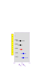
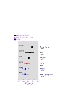
Figure 5: SU(3) breaking ratio of the bag parameters and $B_{B_{d}}^{\overline{\rm MS}}(m_{b})$, as obtained from the lattice studies by extrapolating from the accessible propagating heavy quarks, by constraining the extrapolation with the static HQET result, and by using the NRQCD treatment of the heavy quark. The plotted results are taken from refs. [48, 49, 8, 50, 28, 52].

In fig. 5, we show the results for the SU(3) breaking ratio of the bag parameter, as well as the absolute value of $B_{B}(m_{b})$ in the ${\overline{\rm MS}}$(NDR) scheme. Let us briefly discuss some important points. In ref. [50], the static HQET result has been combined with the ones obtained with the propagating heavy quarks. That was an important progress because, instead of extrapolating, one could interpolate to get the desired result. In doing so the matching of the QCD results with the static (HQET) ones has been made at NLO in perturbation theory, which is important for two reasons:(1) the anomalous dimensions and mixing patterns are different in the full and effective theories (QCD and HQET), and to use the heavy quark scaling laws the matching to HQET is required; (2) to cancel the scale and scheme dependence against the perturbatively computed Wilson coefficient [51] [i.e. $C_{B}(\mu)$ in eq. (1)], one has to provide $B_{B_{s,d}}(\mu)$, computed in the same ${\overline{\rm MS}}$(NDR) renormalization scheme. All schemes are equal at the leading order, and to specify the renormalization scheme, one must go beyond, i.e. to NLO. All that is done consistently in ref. [50]. However, those results are quenched, they are obtained at a single value of the lattice spacing, and the matrix elements in HQET were renormalized only perturbatively. Important step in taming the quenching effects has been made in refs. [28, 52], where the heavy quark is treated non-relativistically. From the comparison of the results obtained in simulations with $N_{\rm f}=0$ and $N_{\rm f}=2$, they see no difference between $B_{B_{d/s}}^{N_{\rm f}=0}$ and $B_{B_{d/s}}^{N_{\rm f}=2}$.

We should reiterate that the light quark in $B_{B_{s}}(\mu)$ is accessed directly, whereas $B_{B_{d}}(\mu)$ is reached through an extrapolation. ChPT suggests no deviation of the SU(3) breaking ratio from the linear form. From ref. [38] we know that the chiral log term reads

$${\hat{B}_{B_{s}}\over\hat{B}_{B_{d}}}=1+{\overbrace{1-3{\hat{g}}^{2}}^{\displaystyle{tiny!}}\over 2(4\pi f)^{2}}\left[m_{\pi}^{2}\log m_{\pi}^{2}-m_{\eta}^{2}\log m_{\eta}^{2}\right]\;,$$ (54)

which, contrary to the case of the decay constants, is very small; no significant shift in the chiral limit is therefore to be expected. That gives us confidence that the chiral extrapolations do not induce important systematic uncertainties, although that issue will be resolved iff we are able to actually do the lattice computation close to the chiral limit. By taking the simple average of the results given in fig. 5, we obtain $B_{B}^{\overline{\rm MS}}(m_{b})=0.89(3)$, to which we add $10\%$ of uncertainty due to possible remaining: quenching, chiral extrapolation, continuum extrapolation effects. To convert from ${\overline{\rm MS}}$ to RGI form, with $\Lambda_{\rm QCD}^{(5)}=213(32)$ MeV [53], the conversion factor in $\hat{B}_{B_{d/s}}=c(m_{b})B_{B_{d/s}}(m_{b})$, is $c^{\overline{\rm MS}}(4.8\ {\rm GeV})=1.54(1)$. The average SU(3) breaking ratio of the bag parameters gives $1.00(1)$, the error of which we double for the same reasons mentioned above. Therefore we have

Since there is still much room for the improvement of the bag parameter results, I should also mention the recent QCDSR result, $B_{B}^{\overline{\rm MS}}(m_{b})\sim 0.95$ [46], as well as the one of the chiral quark model, $B_{B_{s}}/B_{B_{d}}=0.93(5)$ [54]. 

6 $\hat{g}$ coupling

The coupling of the lowest lying doublet of heavy–light mesons ($j_{\ell}^{P}=1/2^{-}$) to a charged soft pion, $g_{H^{\ast}H\pi}$, is defined as

$$\langle H(p^{\prime})\pi(q)|H^{\ast}(p)\rangle=g_{H^{\ast}H\pi}\ \left(q\cdot\varepsilon(p)\right)\;.$$ (56)

This coupling appears to be the essential parameter in the chiral Lagrangian of the heavy–light meson systems, ${\cal L}_{\rm int}=\hat{g}{\rm Tr}[\bar{H}H\gamma_{\mu}\gamma_{5}{\bf A}^{\mu}]$, with $\hat{g}\propto g_{H^{\ast}H\pi}$. The constant $g_{H^{\ast}H\pi}$ is important in describing the $D\to\pi\ell\nu$ and $B\to\pi\ell\nu$ decay form factors, since the residuum of the dominant form factor at the nearest pole (i.e. $m_{D^{\ast}}^{2}$ and $m_{B^{\ast}}^{2}$, respectively) is given by $f_{H^{\ast}}m_{H^{\ast}}g_{H^{\ast}H\pi}/2$. The value of this coupling has recently been measured by CLEO in the charm sector, $g_{D^{\ast}D\pi}=17.9\pm 0.3\pm 1.9$ [55], which we then convert into the value that is expected to scale with the heavy quark mass as a constant (up to $1/m_{Q}$ corrections and higher), namely

$$g_{D^{\ast}D\pi}={2\sqrt{m_{D}m_{D^{\ast}}}\over f_{\pi}}\hat{g}_{c},\quad\hat{g}_{c}^{\rm exp.}=0.59(7)\,,$$ (57)

where the index “$c$” indicates that the heavy quark is charm; $\hat{g}_{b}$, on the other hand, cannot be measured directly because there is no available phase space for the pion emission (or absorption). A summary of the predictions of this quantity as obtained by using various approaches can be found in ref. [56]. Here I will focus on the recent development.

The experimental finding by CLEO was surprising in that the value for $g_{D^{\ast}D\pi}$ was much larger than the one predicted by the light cone QCD sum rules (LCSR) [57]. To cure that discrepancy, ref. [58] proposed to include the first radial excitations in the hadronic sum, i.e. below the continuum threshold in the double dispersion relation. As a result, the LCSR value for $g_{D^{\ast}D\pi}$ becomes much larger and more stable against the variation of the sum rule parameters. In addition, the sum rule for the $D^{(\ast)}$-meson decay constant remains unchanged, whereas the $D\to\pi\ell\nu$ form factor gets corrected in such a way that the result of pole dominance becomes closer to the experimental value for this form factor.

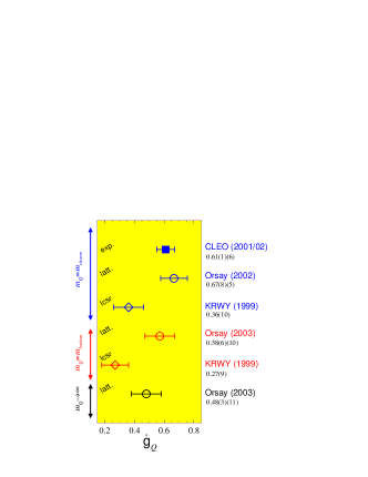
Figure 6: Present situation of the estimates of the $\hat{g}$-coupling between the lowest doublet of heavy–light mesons and the pion. Plotted are the results obtained by using the light cone QCD sum rules (LCSR) [57], (quenched) lattice QCD [59, 61] and the experimental value [55].

The first lattice computation of this coupling was made last year [59]. The findings of that reference can be summarized as follows:

• From the simulations in the quenched approximation, it appears that the finite lattice spacing and finite volume effects are small;

• The coupling is computed from the transition form factor between the light quarks in $H$ and $H^{\ast}$, via the axial current, with the heavy quark being only a spectator. The coupling $\hat{g}_{Q}$ is almost insensitive to the value of the heavy quark mass for the heavy masses around the charm quark (see fig.5 of ref. [59]);

• The resulting value is $\hat{g}_{c}=0.67(8)(^{+4}_{-6})$, i.e. it is large and in good agreement with $\hat{g}_{c}^{\rm exp.}$.

Concerning point 2, the observation that the slope in

$$\hat{g}_{Q}=\hat{g}_{\infty}\ \left(1+\gamma/m_{Q}\right)\;$$ (58)

is $\gamma^{\rm latt}\approx 0$, disagrees with the LCSR prediction, $\gamma^{\rm lcsr}\approx 0.6$ GeV. It is important to say that LCSR came to that conclusion by computing the couplings $\hat{g}_{b}$ and $\hat{g}_{c}$, while on the lattice only the masses close to the charm quark are studied. Since $\hat{g}_{b}$ is highly important [see e.g. eq. (37)], it is necessary to have a better control of the slope $\gamma$. To get around that problem, the Orsay group very recently followed the strategy of ref. [60] and computed $\hat{g}$ on the lattice in the static limit of HQET.  Orsay group obtains $\hat{g}_{\infty}=0.48(3)(10)$, where the bulk of systematic uncertainty stems from various ways of smearing the source operators (the ones that produce $H^{(\ast)}$) [61]. Thus the result for the slope is very close to the one predicted by LCSR, $\gamma^{\rm lcsr}$, although the absolute value obtained on the lattice and from LCSR do disagree. With the static result in hand, one can interpolate to the $B$-meson mass, which results in $\hat{g}_{b}=0.58(6)(10)$.  The present situation of the estimates based on LCSR and quenched lattice simulations is shown in fig. 6. Besides the obvious necessity to go beyond quenching and to better control the chiral extrapolations, it would be nice if other lattice groups produced results for this coupling, even in the quenched approximation.

References

- [1] M. Ciuchini et al., JHEP 0107 (2001) 013, A. Hocker et al., Eur. Phys. J. C 21 (2001) 225.
- [2] M. Battaglia et al., “The CKM matrix and the unitarity triangle,” hep-ph/0304132.
- [3] For a review and references, see Y. Nir, Nucl. Phys. Proc. Suppl. 117 (2003) 111.
- [4] M. Jamin and B. O. Lange, Phys. Rev. D 65 (2002) 056005.
- [5] B. V. Geshkenbein, hep-ph/0309122.
- [6] B. L. Ioffe and K. N. Zyablyuk, Eur. Phys. J. C 27 (2003) 229.
- [7] C. W. Bernard et al., Phys. Rev. D 38 (1988) 3540; M. B. Gavela et al., Phys. Lett. B 206 (1988) 113; C. Alexandrou et al., Phys. Lett. B 256 (1991) 60; A. Abada et al., Nucl. Phys. B 376 (1992) 172; C. W. Bernard, J. N. Labrenz and A. Soni, Phys. Rev. D 49 (1994) 2536; R. M. Baxter et al., Phys. Rev. D 49 (1994) 1594; S. Aoki et al., Nucl. Phys. Proc. Suppl. 47 (1996) 433; T. Bhattacharya and R. Gupta, Phys. Rev. D 54 (1996) 1155; C. R. Allton et al., Phys. Lett. B 405 (1997) 133; C. W. Bernard et al., Phys. Rev. Lett. 81 (1998) 4812; D. Becirevic et al., Phys. Rev. D 60 (1999) 074501; K. C. Bowler et al., Nucl. Phys. B 619 (2001) 507.
- [8] L. Lellouch and C. J. Lin, Phys. Rev. D 64 (2001) 094501.
- [9] A. Juttner and J. Rolf [ALPHA Collaboration], Phys. Lett. B 560 (2003) 59.
- [10] E. Eichten and B. Hill, Phys. Lett. B 234 (1990) 511.
- [11] S. Hashimoto, Phys. Rev. D 50 (1994) 4639; A. Duncan et al., Phys. Rev. D 51 (1995) 5101.
- [12] G. P. Lepage et al., Phys. Rev. D 46 (1992) 4052.
- [13] A. X. El-Khadra, A. S. Kronfeld and P. B. Mackenzie, Phys. Rev. D 55 (1997) 3933.
- [14] A. S. Kronfeld, hep-lat/0205021; C. Davies, hep-ph/0205181.
- [15] J. Flynn, Nucl. Phys. Proc. Suppl. 53 (1997) 168; T. Onogi, ibid 63 (1998) 59; T. Draper, ibid 73 (1999) 43; S. Hashimoto, ibid 83 (2000) 3; C. W. Bernard, ibid 94 (2001) 159; S. M. Ryan, ibid 106 (2002) 86; N. Yamada, hep-lat/0210035.
- [16] M. Guagnelli, F. Palombi, R. Petronzio and N. Tantalo, Phys. Lett. B 546 (2002) 237.
- [17] G. M. de Divitiis et al., hep-lat/0307005, hep-lat/0305018.
- [18] J. Heitger, M. Kurth and R. Sommer, Nucl. Phys. B 669 (2003) 173.
- [19] M. Lüscher et al., Nucl. Phys. B 384 (1992) 168.
- [20] M. Della Morte et al., hep-lat/0307021.
- [21] A. Hasenfratz and F. Knechtli, Phys. Rev. D 64 (2001) 034504, hep-lat/0103029.
- [22] J. Rolf et al., hep-lat/0309072.
- [23] S. Duane et al., Phys. Lett. B 195 (1987) 216; S. Gottlieb et al., Phys. Rev. D 35 (1987) 2531.
- [24] M. J. Peardon, Nucl. Phys. Proc. Suppl. 106 (2002) 3; R. Frezzotti et al., Comput. Phys. Commun. 136 (2001) 1.
- [25] F. Farchioni et al., Eur. Phys. J. C 26 (2002) 237.
- [26] A. Ali Khan et al., Phys. Rev. D 64 (2001) 054504.
- [27] K. I. Ishikawa et al., Phys. Rev. D 61 (2000) 074501.
- [28] S. Aoki et al., hep-ph/0307039.
- [29] A. Ali Khan et al., Phys. Rev. D 64 (2001) 034505.
- [30] C. Bernard et al., Phys. Rev. D 66 (2002) 094501.
- [31] T. Takaishi and P. de Forcrand, Int. J. Mod. Phys. C 13 (2002) 343; S. Aoki et al., Phys. Rev. D 65 (2002) 094507.
- [32] M. Wingate et al., Phys. Rev. D 67 (2003) 054505; preliminary unquenched results are reported in hep-lat/0309092.
- [33] H. Leutwyler, Phys. Lett. B 378 (1996) 313.
- [34] C. Bernard et al., hep-lat/0209163.
- [35] M. J. Booth, Phys. Rev. D 51 (1995) 2338; S. R. Sharpe and Y. Zhang, Phys. Rev. D 53 (1996) 5125.
- [36] N. Yamada et al., Nucl. Phys. Proc. Suppl. 106 (2002) 397; A. S. Kronfeld and S. M. Ryan, Phys. Lett. B 543 (2002) 59.
- [37] L. Giusti, M. Lüscher, P. Weisz and H. Wittig, hep-lat/0309189.
- [38] B. Grinstein et al., Nucl. Phys. B 380 (1992) 369.
- [39] J. J. Sanz-Cillero, J. F. Donoghue and A. Ross, hep-ph/0305181.
- [40] D. Becirevic, S. Fajfer, S. Prelovsek and J. Zupan, Phys. Lett. B 563 (2003) 150.
- [41] K. Hagiwara et al., Phys. Rev. D 66 (2002) 010001.
- [42] D. Becirevic, V. Lubicz and C. Tarantino, Phys. Lett. B 558 (2003) 69 and JHEP 0305 (2003) 007.
- [43] S. Aoki et al., Phys. Rev. D 68 (2003) 054502.
- [44] J. Gasser and H. Leutwyler, Nucl. Phys. B 250 (1985) 465.
- [45] A. Khodjamirian, T. Mannel and M. Melcher, hep-ph/0308297.
- [46] J. G. Korner, A. I. Onishchenko, A. A. Petrov and A. A. Pivovarov, hep-ph/0306032.
- [47] D. Becirevic and J. Reyes, hep-lat/0309131.
- [48] C. W. Bernard, T. Blum and A. Soni, Phys. Rev. D 58 (1998) 014501.
- [49] D. Becirevic et al., Nucl. Phys. B 618 (2001) 241.
- [50] D. Becirevic et al., JHEP 0204 (2002) 025 and Nucl. Phys. Proc. Suppl. 106 (2002) 385.
- [51] G. Buchalla, A. J. Buras and M. E. Lautenbacher, Rev. Mod. Phys. 68 (1996) 1125.
- [52] S. Aoki et al., Phys. Rev. D 67 (2003) 014506.
- [53] S. Bethke, hep-ex/0211012.
- [54] A. Hiorth and J. O. Eeg, hep-ph/0304247, and Eur. Phys. J. directC 30 (2003) 006.
- [55] S. Ahmed et al., Phys. Rev. Lett. 87 (2001) 251801, A. Anastassov et al., Phys. Rev. D 65 (2002) 032003.
- [56] P. Singer, Acta Phys. Polon. B 30 (1999) 3849, D. Becirevic and A. Le Yaouanc, JHEP 9903 (1999) 021.
- [57] A. Khodjamirian, R. Rückl, S. Weinzierl and O. I. Yakovlev, Phys. Lett. B 457 (1999) 245; see also the discussion in A. Khodjamirian, eConf C0304052 (2003) WG504.
- [58] D. Becirevic et al., JHEP 0301 (2003) 009.
- [59] A. Abada et al., Phys. Rev. D 66 (2002) 074504.
- [60] G. M. de Divitiis et al., JHEP 9810 (1998) 010.
- [61] A. Abada et al., hep-lat/0310050.