A Coulomb Gauge Model of Mesons

Abstract

A model of mesons which is based on the QCD Hamiltonian in Coulomb gauge is presented. The model relies on a novel quasiparticle basis to improve the reliability of the Fock space expansion. It is also relativistic, yields chiral pions, and is tightly constrained by QCD (quark masses are the only parameters). Applications to hidden flavor mesons yield results which are comparable to phenomenological constituent quark models while revealing the limitations of such models.

I Introduction

The successes of the quark model of the 1960’s led directly to the development of QCD in the early 1970’s. A central feature of the early quark model was the use of constituent quarks as the relevant degrees of freedom of matter fields. Although the advent of QCD changed the details – the “light” constituent quarks of Copley, Karl, and Obryk have become standard and one gluon exchange is typically employed to describe short range dynamics – the concept of constituent quarks has remained productive and pervasive.

QCD also indicates where the quark model may fail. The canonical nonrelativistic quark model relies on a potential description of quark dynamics and therefore neglects many-body effects in QCD. Related to this is the question of the reliability of nonrelativistic approximations, the importance of hadronic decays, and the chiral nature of the pion. The latter two phenomena depend on the behavior of nonperturbative glue and as such are crucial to the development of robust models of QCD and to understanding soft gluodynamics. Certainly, one expects that gluodynamics will make its presence felt with increasing insistence as experiments probe higher excitations in the spectrum. Similarly the chiral nature of the pion cannot be understood in a fixed particle number formalism. This additional complexity is the reason so few models attempt to derive the chiral properties of the pion. This is an unfortunate situation since the pion is central to much of hadronic and nuclear physics.

To make progress one must either resort to numerical experiments or construct models which are closer to QCD. Here we present one such model which is based on the QCD Hamiltonian in Coulomb gauge. The Hamiltonian approach is appropriate for an examination of the bound state problem because the familiar machinery of quantum mechanics may be employed and because all degrees of freedom are physical in Coulomb gauge. Furthermore, an explicit time-independent potential exists which permits the construction of bound states in a fixed Fock sector. The model consists of a truncation of QCD to a set of diagrams which capture the infrared dynamics of the theory. The efficiency of the truncation is enhanced through the use of quasiparticle degrees of freedom, as will be explained subsequently. Finally, the random phase approximation (RPA) is used to obtain mesons. This many-body truncation is sufficiently powerful to generate Goldstone bosons and has the advantage of being a relativistic truncation of QCDRS .

Because the Hamiltonian is derived from a local density it is covariant, although the use of Coulomb gauge hides this. The truncations which we will employ do not ruin this property. We remark that covariance requires a combination of boost and gauge transformations in noncovariant gauges and therefore some care must be taken in the computation of quantities such as form factors or heavy meson decay rates. Here we focus on static meson properties in the rest frame where these issues do not arise. Finally, we note that maintaining relativistic invariance in schemes which extend the RPA may be difficult because the interaction is no longer instantaneous at higher order. Thus different terms must be summed to yield covariant results and amplitudes may arise which do not have simple wavefunction, or RPA, analogues such as amplitudes with a mixture of forward and backward moving particles.

Using a single framework to generate chiral symmetry breaking and the meson spectrum consistently has been attempted before. LeYaouanc et al. LeYaouanc:1984dr solved a simple gap equation with a quadratic interaction and then used the RPA approximation to obtain chiral pions. Although the interaction is unrealistic it allowed the important simplification of turning integral equations into simple differential equations. Llanes-Estrada and Cotanch LC also studied low-lying states with a linear potential while ignoring state mixing. Neither paper considered the effects of the one gluon exchange potential or renormalization.

An extensive literature on relativistic quark models (which do not consider chiral symmetry breaking) exists. For example, a preliminary study of Fock sector mixing in a relativistic quark model was performed by Koniuk and ZhangZK . Detailed examinations of meson and baryon properties have been carried out by the Bonn groupbonn in a Salpeter equation framework with a model confinement potential and Dirac structure. Similarly, extensive computations of pion and kaon properties have been carried out in a covariant Euclidean space Dyson-Schwinger formalismMR .

Finally, the gluonic portion of the formalism presented here has been used to derive the quenched positive charge conjugation glueball spectrumss8 . The results are in very good agreement with lattice computations, indicating that the method has some promise.

II Model Definition: the Quark Vacuum and Chiral Symmetry Breaking

Generating the meson spectrum proceeds in three steps: (1) a quasiparticle basis for the gluonic sector of QCD is obtained with standard many-body techniques, (2) this procedure yields an instantaneous interaction which is used to construct a quasiparticle (constituent) basis in the quark sector, (3) bound state properties are obtained in the the random phase approximation. The first step contains an important complication: the quasiparticle interaction of QCD depends on the quasiparticles themselves (in a way made clear below) and hence must be solved along with the gap equation. This allows the possibility of deriving the constituent quark interaction if one can obtain the functional form of the interaction. We note that this is similar to solving coupled Dyson-Schwinger equations for, say, the gluon propagator and vertices.

II.1 QCD in Coulomb Gauge

The Coulomb gauge QCD Hamiltonian may be written as $H_{QCD}=H_{0}+H_{int}$ withCL ; schwinger ; ss7

$$H_{0}=\int\psi^{\dagger}\left(-i\bm{\alpha}\cdot{\mbox{\boldmath$\nabla$}}+\beta m\right)\psi+{1\over 2}\int d{\bf x}\left(\bm{\Pi}^{2}-{\bf A}{\mbox{\boldmath$\nabla$}}^{2}{\bf A}\right)+{1\over 2}\int d{\bf x}d{\bf y}\,\rho^{a}({\bf x})K^{(0)}({\bf x}-{\bf y})\rho^{a}({\bf y})\ \ .$$ (1)

The interaction term contains the familiar transverse gluon color charge interaction and all of the higher order terms due to the non-Abelian nature of QCD:

$$H_{int} ={1\over 2}\int d{\bf x}\left[{\bf B}^{2}+{\bf A}{\mbox{\boldmath$\nabla$}}^{2}{\bf A}\right]-g\int\psi^{\dagger}\bm{\sigma}\cdot{\bf A}\psi+V_{A}+V_{B}+$$ (2)

$$+{1\over 2}\int d{\bf x}d{\bf y}\,\rho^{a}({\bf x})\left[K^{ab}({\bf x}-{\bf y};{\bf A})-\delta^{ab}K^{(0)}({\bf x}-{\bf y})\right]\rho^{b}({\bf y})$$

The density $\rho^{a}$ entering these equations is the full color charge due to quarks and gluons

$$\rho^{a}({\bf x})=f^{abc}{\bf A}^{b}({\bf x})\cdot\bm{\Pi}^{c}({\bf x})+\psi^{{\dagger}}({\bf x}){\lambda^{a}\over 2}\psi({\bf x}).$$ (3)

The instantaneous non-Abelian Coulomb interaction in Eq. 2 is given by

$$K^{ab}({\bf x},{\bf y};{\bf A})\equiv\langle{\bf x},a|{g\over{{\mbox{\boldmath$\nabla$}}\cdot{\bf D}}}(-{\mbox{\boldmath$\nabla$}}^{2}){g\over{{\mbox{\boldmath$\nabla$}}\cdot{\bf D}}}|{\bf y},b\rangle,$$ (4)

where ${\bf D}$ is the covariant derivative in adjoint representation

$${\bf D}^{ab}=\delta^{ab}{\mbox{\boldmath$\nabla$}}-gf^{abc}{\bf A}^{c}.$$ (5)

The electric and magnetic fields are defined by

$$\Pi^{a}\equiv-{\bf E}_{tr}^{a}=\dot{\bf A}^{a}+g(1-{\mbox{\boldmath$\nabla$}}^{-2}{\mbox{\boldmath$\nabla$}}{\mbox{\boldmath$\nabla$}}\cdot)f^{abc}A^{0b}{\bf A}^{c}$$ (6)

and

$${\bf B}^{a}={\mbox{\boldmath$\nabla$}}\times{\bf A}^{a}+{1\over 2}gf^{abc}{\bf A}^{b}\times{\bf A}^{c}.$$ (7)

The interaction in $H_{0}$ is defined as the vacuum expectation value of the Coulomb interaction

$$\delta^{ab}K^{(0)}({\bf x}-{\bf y})=\langle\Psi_{0}|K^{ab}({\bf x},{\bf y};{\bf A})|\Psi_{0}\rangle.$$ (8)

The vacuum state will be defined shortly.

Finally, the imposition of Coulomb gauge restricts the theory to a curved gauge manifold with a metric given by $\langle\Phi|\Psi\rangle=\int{\cal D}{\bf A}{\cal J}[{\bf A}]\Phi^{*}({\bf A})\Psi({\bf A})$. The factor ${\cal J}$ is the Faddeev-Popov determinant given by

$${\cal J}={\rm det}({\mbox{\boldmath$\nabla$}}\cdot{\bf D}).$$ (9)

The Faddeev-Popov determinant may be removed from the metric by rescaling the Hamiltonian

$$H\to{\cal J}^{1/2}H{\cal J}^{-1/2}$$

which is hermitian with respect to $(\Phi|\Psi)=\int{\cal D{\bf A}}\Phi^{*}({\bf A})\Psi({\bf A})$. We note that the nontrivial metric induces two new terms, denoted $V_{A}$ and $V_{B}$, which correspond to the anomalous terms of Schwingerschwinger ; CL .

It has been speculated that confinement is related to the well-known Gribov ambiguitygribov ; Z . The Gribov ambiguity arises because the existence of topologically inequivalent solutions to the gauge condition ${\mbox{\boldmath$\nabla$}}\cdot{\bf A}=0$ implies that the gauge is incompletely specified. Gribov proposed that the ambiguities with Coulomb gauge may be resolved by considering fields with $\det({\mbox{\boldmath$\nabla$}}\cdot{\bf A})\geq 0$ which comprise the ‘Gribov region’ (GR). We note that the appearance of the inverse of the Faddeev-Popov operator in the instantaneous Coulomb potential implies that gauge configurations near the boundary of the Gribov region create a strong infrared enhancement in the interaction. It is possible that this enhancement is the origin of confinement in Coulomb gaugeZ .

Subsequent research has shown that the Gribov region actually contains gauge copies and hence gauge fields must lie in a subset of the Gribov region called the fundamental modular region (FMR). The FMR contains no redundant field configurations and may be defined, for example, as the set of global minima over gauge transformations of the functional

$$F_{\bf A}[g]={\rm Tr}\int d^{3}x({\bf A}^{g})^{2}$$ (10)

where ${\bf A}^{g}=g{\bf A}g^{\dagger}-g{\mbox{\boldmath$\nabla$}}g^{\dagger}$. It is now known that the FMR contains the GR except at certain points where the regions coincide, the FMR is convex, and the GR contains the originvanbaal . Furthermore, Zwanziger has recently arguedZ3 that observables have their support over the intersection of the FMR and the GR, thereby resurrecting the infrared enhancement argument of the previous paragraph. Finally, topological aspects of QCD may be introduced to the formalism via the imposition of wavefunctional boundary conditions on the boundary of the FMRvanbaal .

II.2 Gluon Gap Equation and the Instantaneous Interaction

It is clear that the interaction of quarks is strongly influenced by the instantaneous Coulomb interaction of Eq. 4. It is known, moreover, that the instantaneous interaction is renormalization group invariantZ . This fact permits a physical interpretation of the instantaneous potential which is a central aspect of our formalism. Furthermore, Zwanziger has shown that the Coulomb interaction provides an upper bound to the Wilson loop potential and has postulated that this bound is, in fact, saturatedZ1 . We remark that this saturation is crucial to the formalism presented here. This postulate may be checked with lattice computations, unfortunately the results are mixed ZC ; G . If the evidence to the contrary is confirmed, this approach must be abandoned.

The nonpolynomial functional dependence of the Coulomb interaction on the vector potential complicates computations in Coulomb gauge. We proceed by separating the interaction into two parts denoted by $K^{(0)}$ (see Eq. 8) and $K-K^{(0)}$. Since $K^{(0)}$ is a vacuum expectation value it contains all diagrams in which gluons are attached to the operator $\rho K\rho$. Thus the remainder necessarily contains gluons which propagate. Since gluons are quasiparticles with a dynamical mass on the order of 1 GeV (the hybrid-meson mass gap), matrix elements of $K-K^{(0)}$ are suppressed in typical hadronic observables, considerably simplifying computations.

In spite of this, it is impossible to obtain a closed form expression for the the vacuum expectation value of $K$. However, a procedure for obtaining Dyson equations which sum the leading infrared diagrams for this matrix element has been described in Ref.ss7 . An important element in the formalism is the construction of a basis which permits an efficient Fock space expansion. The method proposed in Ref. ss7 built this basis with the aid of a gluonic vacuum Ansatz (it is worth stressing that the vacuum need not be highly accurate, it merely provides a starting point for constructing a more general quasiparticle basis, and any sufficiently general vacuum Ansatz will suffice). The Ansatz employed is

$$\Psi_{0}[{\bf A}]=\langle{\bf A}|\omega\rangle=\exp\left[-{1\over 2}\int d{\bf k}{\bf A}^{a}({\bf k})\,\omega(k){\bf A}^{a}(-{\bf k})\right].$$ (11)

which depends on an unknown trial function, $\omega(k)$. This is the simplest correlation one can build into the vacuum and corresponds to the BCS Ansatz of many-body physics. Note that the perturbative vacuum is obtained when $\omega=|{\bf k}|$.

The trial function is obtained by minimizing the vacuum energy density

$${{\delta}\over{\delta\omega}}\langle\omega|H|\omega\rangle=0.$$ (12)

The vacuum state obtained from this procedure is denoted $|\omega\rangle$. We refer to $\omega$ as the gap function since it is also responsible for lifting the single particle gluon energy beyond its perturbative value. Of course evaluating the matrix element in Eq. 12 requires an explicit expression for $\langle\omega|\rho K\rho|\omega\rangle$ which is provided by the Dyson procedure described above. The result is a set of coupled nonlinear integral equations which describe the gap equation and the Dyson equation for $K^{(0)}$. Solving these equations yields both the quasigluon dispersion relation, $\omega(k)$, and the quasigluon effective interaction, $K^{(0)}({\bf x}-{\bf y})$. Renormalization is achieved by fitting the latter to the lattice Wilson loop potential. The result is in excellent agreement with the lattice and provides a dynamical mass scale for the quasigluons: $m_{g}\equiv\omega(0)\approx 600$ MeV. It is this large mass scale which permits rapid convergence of any Fock series expansion in the gluonic sector of QCD and explains why quark degrees of freedom dominate low energy hadronic physics. We remark that the emergence of a confining potential is nontrivial and indicates the robustness of the method.

An analytic approximation to the solution to the coupled equations yields the following form for the vacuum expectation value of the Coulomb interactionss7 :

$$K^{(0)}(k)={12.25\over k^{2}}\left\{\begin{array}[]{ll}\left({m_{g}\over k}\right)^{1.93}&k<m_{g}\\ {0.6588\log(k^{2}/m_{g}^{2}+0.82)^{-0.62}\log(k^{2}/m_{g}^{2}+1.41)^{-0.80}}&k>m_{g}\end{array}\right.$$ (13)

This form mimics the numerical solution and the lattice results quite well. The long range potential behaves as $k^{-3.93}$, within 2% of the expected linear behavior (the deviation is likely to be a numerical artifact). This allows the extraction of a string tension via $6\pi b\approx 12.25m_{g}^{2}$, which implies $b\approx 0.234$ GeV². The effect of the smaller exponent is to reduce this string tension to approximately 0.21 GeV² at physically relevant scales. A fit to the standard ‘Coulomb plus linear’ potential (const - $4/3\cdot\alpha_{s}/r+br$) yields an effective strong coupling of $\alpha_{s}=0.12$. This value is rather small with respect to expectations (in part because there was little lattice data at small distances in the fit of Ref.ss7 ). Thus we have also employed a modified potential of the form

$$K^{(0)}(k)={12.25\over k^{2}}\left\{\begin{array}[]{ll}\left({m_{g}\over k}\right)^{1.93}&k<m_{g}\\ \left({\log(1+a)\over\log(k^{2}/m_{g}^{2}+a)}\right)^{b}&k>m_{g}\end{array}\right.$$ (14)

Here $a$ and $b$ are constants which may be varied. Values of $a=1.0$ and $b=0.8$ give a potential which agrees well with lattice data at short distance, but which otherwise is very close to the original form of Eq.13. Both potentials have been employed in the following to test the sensitivity of the results on the functional form of the potential.

II.3 Quark Gap Equation

Our chief goal is to examine a model of QCD which permits the simultaneous description of heavy quarkonia and chiral pions. It is clear that this may not be achieved in a potential formalism – the many-body aspect of QCD is required. Our approach to the quark sector therefore mimics that of the gluon sector, namely we model the quark vacuum with a Gaussian wavefunctional and determine the quark gap equation. Solving this yields dynamical chiral symmetry breaking and a massless Goldstone boson in the random phase approximation in accord with the Thouless sum rulethouless . We note that this general approach has been used many times in the past, starting with the classic work of Nambu and Jona-Lasinio NJL . Subsequent work has dealt with renormalization issues A ; FM or with models which are closer to QCD Orsay . How the constituent quark model may be reconciled with chiral symmetry breaking is explained in Ref. ss5 . Finally an extensive literature on the Dyson-Schwinger approach to this problem existsMR .

In this approach the gap equation represents a nonperturbative one loop computation and thus must be properly renormalized. As noted in the gluonic sector, this is a nontrivial step whose implementation depends on the subset of diagrams being summed. In the BCS/RPA formalism employed here, we have found that standard renormalization is sufficient to guarantee finite results. In particular we have added mass renormalization

$$\delta H_{m}=\delta m\int d{\bf x}\,\psi^{\dagger}\beta\psi$$

and wavefunction renormalization

$$\delta H_{\psi}=\left(Z_{\psi}-1\right)\int d{\bf x}\,\psi^{\dagger}(-i{\bm{\alpha}}\cdot{\mbox{\boldmath$\nabla$}})\psi$$

terms to the Hamiltonian of Eq. 1 and the theory has been truncated at the scale $\Lambda$. Recall that the effective instantaneous interaction has already been rendered finite.

Proceeding with the standard Bogoliubov or Dyson procedure yields the following quark gap equation

$$Z_{\psi}(\Lambda)ps_{p}=\left[m(\Lambda)+\delta m(\Lambda)\right]c_{p}+{C_{F}\over 2}\int{k^{2}dk\over(2\pi)^{3}}\left[V_{0}(p,k)s_{k}c_{p}-V_{1}(p,k)c_{k}s_{p}\right]$$ (15)

where

$$V_{L}(p,k)=2\pi\int d(\hat{p}\cdot\hat{k})\,K^{(0)}({\bf p}-{\bf k})P_{L}(\hat{p}\cdot\hat{k}).$$

The functions $s_{k}$ and $c_{k}$ are defined in terms of the Bogoliubov angle $\phi(k)$ as $s_{k}=\sin\phi(k)$ and $c-k=\cos\phi(k)$. The quark gap equation is to be solved for the unknown Bogoliubov angle, which then specifies the quark vacuum and the quark field mode expansion via spinors of the form

$$u_{s}(k)=\sqrt{1+s_{k}\over 2}\left(\begin{array}[]{c}\chi_{s}\\ {c_{k}\over 1+s_{k}}{\bm{\sigma}\cdot\hat{k}}\chi_{s}\end{array}\right).$$ (16)

Comparing the quark spinor to the canonical spinor (we use nonrelativistic normalization) permits a simple interpretation of the Bogoliubov angle through the relationship $\mu(k)=k\tan\varphi(k)$ where $\mu$ may be interpreted as a dynamical momentum-dependent quark mass. Similarly $\mu(0)$ may be interpreted as a constituent quark mass.

In the case of massless quarks the right hand side of the quark gap equation diverges logarithmically for potentials obeying the perturbative relation $K^{(0)}(k)\to k^{-2}$ for large $k$. The divergence may be absorbed into the wavefunction renormalization, $Z_{\psi}=1-C_{F}/(6\pi^{2})\log\Lambda$, yielding a finite gap equation. It is also possible to renormalize by examining the once-subtracted gap equation. For the massive quark case two logarithmic divergences proportional to the quark mass and momentum appear. It is convenient to absorb these divergences separately into the mass and wavefunction terms respectively. For the study presented here the potential is modified by logarithmic corrections at short distances, thus all integrals are finite and the cutoff may be removed immediately. We note, however, that it still may be useful to make finite renormalizations.

The numerical solution for the dynamical quark mass is very accurately represented by the functional form

$$\mu(k)=\sigma K^{(0)}(k)\left(1-{\rm e}^{-{M/(\sigma K^{(0)}(k)})}\right)$$ (17)

where $M$ is a ‘constituent’ quark mass and $\sigma$ is a parameter related to the quark condensate. Notice that this form approaches the constituent mass for small momenta and $\sigma K^{(0)}$ for large momenta. The latter behavior is in accord with the quark gap equation which implies thatP

$$\mu(k)\to{C_{F}\over 2}\int{d^{3}q\over(2\pi)^{3}}K^{(0)}(k)s(q)=-{C_{F}\over 4N_{c}}K^{(0)}(k)\langle\bar{\psi}\psi\rangle.$$ (18)

A rough fit to the numerical solution yields $M=68$ MeV and $\sigma=$ 0.001 GeV³. The constituent quark mass is small compared to typical relativistic constituent quark model masses of roughly 200 MeV. The value for $\sigma$ implies a quark condensate of approximately (-210 MeV)³, in reasonable agreement with current estimates of (-250 MeV)³. However, we note that direct computations of the condensate typically yield results of approximately (-110 MeV)³. These flaws undoubtedly point to inadequacies in the quark vacuum Ansatz. Of course, since we are working with the full QCD Hamiltonian, it is possible to improve the Ansatz (for a coupled cluster approach, see Ref. SK ; for one loop corrections see Ref. ss4 ). Since one of our chief interests is the implementation of a formalism which respects chiral symmetry, and not detailed numerics, we satisfy ourselves with the present procedure.

III Mesons

With explicit expressions for the quasigluon interaction (and hence the constituent quark interaction) and the dynamical quark mass in hand we are ready to obtain mesonic bound states. As mentioned above, in order to obtain a massless pion one must construct states, $|M\rangle$, in the random phase approximation:

$$\langle M|[H,Q^{{\dagger}}_{M}]|RPA\rangle=(E_{M}-E_{BCS})\langle M|Q^{{\dagger}}|RPA\rangle,$$ (19)

where $Q^{{\dagger}}_{M}$ is defined in terms of the positive and negative energy wavefunctions, $Q^{{\dagger}}_{M}=\sum_{\alpha\beta}\left[\psi^{+}_{\alpha\beta}B^{{\dagger}}_{\alpha}D^{{\dagger}}_{\beta}-\psi^{-}_{\alpha\beta}D_{\beta}B_{\alpha}\right]$ with $B$ and $D$ being the quasiparticle operators. It is worthwhile recalling that the RPA method is equivalent to the Bethe-Salpeter approach with instantaneous interactionsRS .

The RPA and TDA equations includes self energy terms (denoted $\Sigma$) for each quark line and these must be renormalized. In the zero quark mass case renormalization of the TDA or RPA equations proceeds in the same way as for the quark gap equation. In fact, the renormalization of these equations is consistent and one may show that a finite gap equation implies a finite RDA or TDA equation. This feature remains true in the massive case.

The RPA equation in the pion channel reads:

$$(E_{\pi}-E_{BCS})\psi^{+}(k) = 2\left[ms_{k}+kc_{k}+\Sigma(k)\right]\psi^{+}(k)$$ (20)

$$-{C_{F}\over 2}\int{p^{2}dp\over(2\pi)^{3}}\left[V_{0}(k,p)(1+s_{k}s_{p})+V_{1}(k,p)c_{k}c_{p}\right]\psi^{+}(p)$$

$$-{C_{F}\over 2}\int{p^{2}dp\over(2\pi)^{3}}\left[V_{0}(k,p)(1-s_{k}s_{p})-V_{1}(k,p)c_{k}c_{p}\right]\psi^{-}(p)$$

A similar equation for $\psi^{-}$ holds with $(+\leftrightarrow-)$ and $E\to-E$. The wavefunctions $\psi^{\pm}$ represent forward and backward moving components of the many-body wavefunction and the pion itself is a collective excitation with infinitely many constituent quarks in the Fock space expansion.

We also consider a simpler truncation of QCD called the Tamm-Dancoff approximation. This may be obtained from the RPA equation by neglecting the backward wavefunction $\psi^{-}$.

We have computed the spectrum in the random phase and Tamm-Dancoff approximations and confirm that the pion is massless in the chiral limit. We also find that the Tamm-Dancoff approximation yields results very close to the RPA for all states except the pion: the TDA pion mass is 580 MeV while the first excited pion has an RPA mass of 1410 MeV and a TDA mass of 1450 MeV. All other mesons have nearly identical RPA and TDA masses. For this reason we simply present TDA equations and results below.

The complete hidden flavor meson spectrum in the Tamm-Dancoff approximation is given by the following equations.

$$E\psi_{PC}(k)=2\left[ms_{k}+kc_{k}+\Sigma(k)\right]\psi_{PC}(k)-{C_{F}\over 2}\int{p^{2}dp\over(2\pi)^{3}}K^{PC}_{J}(k,p)\psi_{PC}(p)$$ (21)

with

$$\Sigma(k)={C_{F}\over 2}\int{p^{2}dp\over(2\pi)^{3}}\left(V_{0}s_{k}s_{p}+V_{1}c_{k}c_{p}\right)$$ (22)

and where $\psi$ is the meson radial wavefunction in momentum space.

An alternate form for the kinetic and self energies which is closer the Schrödinger equation may be obtained by substituting the gap equation to obtain:

$$\mbox{ kinetic + self energy}=2\left[E(k)+\Gamma(k)\right]$$ (23)

where

$$\Gamma(k)={C_{F}\over 2}\int{p^{2}dp\over(2\pi)^{3}}V_{1}{c_{p}\over c_{k}}.$$ (24)

and

$$E(k)=\sqrt{k^{2}+\mu(k)^{2}}.$$ (25)

The kernel, $K_{J}$ in the potential term depends on the meson quantum numbers, $J^{PC}$. In the following possible values for the parity or charge conjugation eigenvalues are denoted by $(J)=+$ if $J$ is even and $-$ if $J$ is odd.

$\bullet\$ $0^{++}$

$$K(p,k)=V_{0}c_{p}c_{k}+V_{1}(1+s_{p}s_{k})$$ (26)

$\bullet\$ $J^{(J+1)(J)}$ [${}^{1}J_{J}$ , $J\geq 0$]

$$K_{J}(p,k)=V_{J}(1+s_{p}s_{k})+\left(V_{J-1}{J\over 2J+1}+V_{J+1}{J+1\over 2J+1}\right)c_{p}c_{k}$$ (27)

$\bullet\$ $J^{(J+1)(J+1)}$ [${}^{3}J_{J}$ , $J\geq 1$]

$$K_{J}(p,k)=V_{J}(1+s_{p}s_{k})+\left(V_{J-1}{J+1\over 2J+1}+V_{J+1}{J\over 2J+1}\right)c_{p}c_{k}$$ (28)

$\bullet\$ $J^{(J)(J)}$ [${}^{3}(J-1)_{J},^{3}(J+1)_{J}$ , $J\geq 1$]

$$K_{11}(p,k) = V_{J}c_{p}c_{k}+\left(V_{J-1}{J\over 2J+1}+V_{J+1}{J+1\over 2J+1}\right)(1+s_{p}s_{k})$$ (29)

$$K_{22}(p,k) = V_{J}c_{p}c_{k}+\left(V_{J-1}{J+1\over 2J+1}+V_{J+1}{J\over 2J+1}\right)(1+s_{p}s_{k})$$ (30)

$$K_{12}(p,k) = \left(V_{J-1}-V_{J+1}\right){\sqrt{J(J+1)}\over 2J+1}\left(s_{k}+s_{p}\right)$$ (31)

These interaction kernels have been derived in the quark helicity basis. We remark that in the LS basis the off-diagonal (J-1):(J+1) interaction for $J^{(J)(J)}$ mesons is proportional to $1+s_{k}s_{p}-s_{k}-s_{p}$ and hence goes to zero in the heavy quark mass limit as expected. Finally, we note that the authors of Ref. LC find that the $1^{++}$ and $1^{+-}$ kernels are identical. The likely reason is an error in their $1^{+-}$ kernel which disagrees with that of Eq. 27.

III.1 Short Range Behavior

Our quark interaction is instantaneous, central, and obeys Casimir scaling. However, it is not flavor or spin independent because the full spinor structure of the interaction has been retained. This spinor structure is specified by the Hamiltonian of QCD and is of a vector nature (specifically $\bar{\psi}\gamma_{0}\psi\otimes\bar{\psi}\gamma_{0}\psi$). A nonrelativistic reduction of this interaction yields no spin-spin hyperfine or tensor interactions. Thus the present computation cannot correctly describe well known spin splittings such as $J/\psi-\eta_{c}$ or $\Delta-N$ (we describe the extensions necessary to do so below).

A spin-orbit interaction is present and is given by

$$V_{SO}={1\over 2m^{2}r}{d\over dr}\left(-C_{F}K^{(0)}(r)\right)\vec{L}\cdot\vec{S}$$ (32)

in the equal quark mass case.

The spin-orbit interaction is famous for its problematic nature in the constituent quark model. Quark model lore states that the spin-orbit interaction generated by one gluon exchange is too strong for phenomenology and must be softened by the addition of a spin orbit interaction from the confinement term which has an opposite sign. This can only be arranged if confinement has a scalar Dirac structure ($\bar{\psi}\psi\otimes\bar{\psi}\psi$). This is clearly at odds with the formalism presented here which insists that the confinement and Coulomb potentials (here we mean the perturbative $1/r$ tail of the static potential) share the same Dirac structure. The resolution to the conundrum is that it is too simple-minded to ascribe all of spin-orbit interactions to the Dirac structure of instantaneous potentials. Indeed, spin-dependence in QCD is partly generated by nonperturbative mixing with intermediate states, and need not follow the dictates of quark model lore. A specific realization of this is given in Ref. ss3 . Finally, we note that a scalar confinement interaction leads to inconsistencies between mesons and baryons: if mesons confine then baryons anticonfine — clearly an unacceptable situation!

Relativistic interactions generate short range spin-dependent interactions by virtue of their spinor structure. The other sources of spin-dependence are topological effects (for example, an instanton induced interaction) and Fock sector mixing effects. Fock sector mixing is easily incorporated into the current formalism, one need only increase the size of the Fock space being considered (there is one subtlety: the mixing between Fock sectors must be treated carefully since it can involve nonperturbative gluodynamics). One expects the leading higher Fock sectors to be meson-meson (ie., meson loop corrections to the spectrum) and hybrid. The latter case is the nonperturbative analogue of one-gluon-exchange, and as mentioned above, is phenomenologically important in the light meson spectrum.

We shall leave the topic of Fock space mixing for a future investigation and press ahead with an examination of the spectrum which arises from the central static potential generated by the non-Abelian Coulomb interaction, keeping in mind that large spin-dependent mass shifts may occur in the light spectrum.

IV Results and Discussion

Once the gluonic sector of the formalism has been fixed by renormalization the only remaining parameters are quark masses. In the following we have determined these by fitting the $\Upsilon$, $J/\psi$, and $\phi$ masses. We work in the chiral limit for light ($u$ and $d$ quark) mesons so predictions in this sector are completely fixed. As a result there is no possibility of adjusting the spectrum presented below. Thus it is possible to test the assumptions of the model throughout the spectrum.

IV.1 Quarkonia

A simple way to obtain the upsilon spectrum from QCD is to insert the lattice Wilson potential into the nonrelativistic Schrödinger equation. One argues that the heavy $b$ quark mass validates the Born-Oppenheimer approximation (so that the static potential may be used) and the use of a nonrelativistic framework. Precisely this approach has been taken by Juge, Kuti, and MorningstarJKM (JKM) and was subsequently justified by comparison with nonrelativistic lattice computationsJKM2 .

Since the potential we employ is essentially equivalent to that obtained from the Wilson loop one may expect that the predicted upsilon spectrum will agree very closely with that of JKM. This expectation relies on two things: (i) the heavy quark mass must eliminate non-central contributions in the interaction kernel, (ii) the self energy contribution must be essentially independent of momentum. (The authors of Ref. JKM did not include a self energy term in their model because it cannot be extracted from lattice data. Such a term must exist as external fermion propagator corrections.) Explicit computations show that these expectations are indeed borne out and indicate that a finite renormalization is sufficient to largely eliminate the self energy term.

Our predicted upsilon spectrum is given in Table I. A comparison with experiment shows that the radial excitations rise too slowly with radial quantum number, and indeed our results similarly disagree with those of JKM. But, as noted above, the form for the static potential of Eq. 13 is not strongly constrained at large momenta. We have therefore computed the upsilon spectrum with the modified potential of Eq. 14. The results are shown in Table II and are in much better agreement with JKM and experiment. As expected, the detailed form of the Coulomb tail of the potential is very important for low-lying heavy quark states. Our results are very similar to typical quark model spectraGI ; with some deviation (at the percent level) becoming visible higher in the spectrum. This is to be expected because we employ a lattice potential with a string tension of 0.2-0.25 GeV² whereas the quark model of Ref. GI takes $b=0.18$ GeV².

Overall, the agreement with the experimental upsilon spectrum is impressive considering the simplicity of the model and that the potential was not fit to data. It is possible that deviations are seen higher in the spectrum, and indeed, one may expect this since the open flavor threshold is at 10.56 GeV – between the third and fourth vector S-wave states. In general mixing with higher Fock components, such as hybrids (one gluon exchange in perturbative language) and meson-meson channels, will occur. These effects should become more important as one probes higher in the spectrum. Eventually the quark + potential picture of mesons should break down entirely as an increasing number of gluonic degrees of freedom are excited.

The psi spectrum predicted with the canonical potential of Eq. 13 is presented in Table III. The agreement with experiment is on the percent level. This is something of a surprise when considering that the upsilon spectrum required a careful fit to the high momentum potential. The psi spectrum computed from the modified potential (Table IV) compares unfavorably to the data, with deviations at the five percent level. It appears that the linear and Coulomb portions of the potential are equally important to the low-lying psi spectrum and that the small value of the effective strong coupling has largely cancelled against the large value of the string tension. Indeed, as mentioned above, quark models typically employ a much smaller string tension than that of the Wilson loop. We thus have evidence that the effective string tension is reduced for lighter quark masses. This can easily be induced by mixing with virtual meson pairs or by motion of the sources in the Wilson loop. Again, it should be possible to incorporate the physics of string softening in the model through Fock sector mixing.

The results of Tables III and IV also indicate that spin splittings are becoming important. For example the $\eta_{c}$ is roughly 100 MeV lighter than the $J/\psi$ and this is not predicted in the model. Again, this fault is easy to remedy once higher Fock components are admitted. One also sees evidence for tensor splitting in the $J^{++}$ states which are quite well reproduced with the modified potential (Table IV). One concludes that the Dirac structure of the interaction is becoming important and that it does a reasonable job at charm mass scales but that Fock mixing must be accounted for, even for low-lying states. As indicated in the Introduction, if canonical quark model lore holds, the addition of virtual hybrid states to the model will ruin the predicted tensor splittings since these will increase them an unacceptable amount. We stress, however, that nonperturbative mixing with virtual hybrid states is not equivalent to perturbative gluon exchange which only becomes relevant in Hamiltonian QCD very high in the spectrum.

IV.2 Isovector Mesons

We have seen that the formalism presented here is quite accurate for bottom quarks and reasonably accurate (with the possibility of being very accurate once simple Fock sector mixing is included) for charm quarks. The challenge in carrying this success to the light quark sector lies in (i) the assumption that the static Wilson loop potential is relevant to light quarks, (ii) the importance of chiral symmetry breaking, (iii) large spin-dependences which may be present, (iv) the possibility that topological aspects of QCD become important. One of the reasons Coulomb gauge QCD is useful for constructing models of hadronic physics is that these issues may be addressed in a systematic fashion. The latter three issues have already been discussed; for the first we note that an instantaneous interaction between quarks exists for all quark masses in Coulomb gauge. The viability of this interaction can only be affected by higher order gluonic terms (such as in the operator $K-K^{(0)}$); but we have seen that these contributions are suppressed by an energy denominator of the order of 1 GeV. Thus a static interaction should provide a good approximation low in the light spectrum. Virtual light quark loops are another source of nonpotential interactions. But chiral symmetry breaking implies that the light current quarks acquire an effective mass, and this mass assists in dampening such loop effects. The success of the constituent quark model also indicates that loop effects on the interaction can be largely subsumed by renormalization.

Our results for the light meson spectrum are presented in Figure 1 and in Table V. The first feature to notice is that the pion is massless as desired. Of course a finite pion mass can be obtained if a finite current quark mass is used in the calculation. We have chosen to keep the current quark mass at zero in order to test the robustness of the model in a zero parameter computation.

The rho meson mass is predicted to be 772 MeV, in very good agreement with data. We regard this as somewhat fortuitous since the potential has been fixed by lattice data and no parameter tuning has taken place. The first radial excitation is at 1390 MeV, whereas the experimental mass is approximately 1450 MeV. However, we note that already the possibility of Fock mixing arises since the lowest mass vector hybrid is expected around 1900 MeV.

As seen in the psi spectrum, the tensor $J^{++}$ multiplet is sensitive to short range effects. In this case the $1^{++}$ state is in rough agreement with experiment. However the tensor state lies much above the data. The isoscalar scalar has a mass of 850 MeV. One may be tempted to ascribe this state to the $f_{0}(980)$, which is famous for being too light in constituent quark models. However, the fact that the tensor state is much too massive is an indication that additional strong spin-orbit forces are required to obtain a satisfactory description of light mesons and that any conclusions concerning the nature of the scalar meson would be premature.

The figure and table also present meson masses for high angular momentum. It is seen that the model severely overestimates the masses of these states. The likely cause for this is the large (compared to quark model) string tension which we have used. However, as argued above, there is little freedom in choosing the string tension and one must ascribe the discrepancy to nonpotential effects. The simplest such effects are extra quasigluons in the Fock space expansion of higher lying states. Thus we regard the poor quality of the predictions at high angular momentum as an indication of the range of validity of the potential approach to hadronic physics (of course it is possible to extend this range by allowing more parameter freedom, but the degrees of freedom will be incorrect, and detailed predictions of such models must fail).

Equations (27) and (28) make it clear that meson masses form charge conjugation doublets in the pattern $1^{+\pm}$, $2^{-\pm}$, etc. in the large angular momentum limit. This pattern is clearly seen in the figure. Such behavior is expected in the heavy quark limit where quark spins decouple and one may expect it to also occur for light quarks in the high angular momentum regime since the quark spin effects are local in the interaction.

A central feature of chiral symmetry breaking is that quark spinors reduce to massless spinors at momenta much larger than the chiral symmetry breaking scale. Thus one has $c_{k}\to 1$ and $s_{k}\to 0$ for $k>>\Lambda_{\chi SB}$. Since the average quark momentum becomes large as the angular momentum increases we conclude that the interaction kernel approaches

$$K_{J}\to V_{J}+{1\over 2}V_{J-1}+{1\over 2}V_{J+1}$$ (33)

for all possible $J^{PC}$ (the off-diagonal potential in the $J^{(J)(J)}$ sector goes to zero). Thus the entire spectrum becomes degenerate in the large angular momentum limit; in particular parity doubling occurs, as expectedCG .

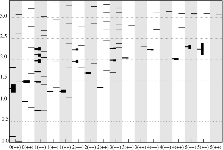
Figure 1: The isovector meson spectrum. Experimental massesPDG are represented by lines to the left of each column. The attached boxes indicate the widths of each state. Lines to the right are the results of this computation in the massless quark limit. Narrower boxes are new results from the Crystal Barrel collaborationCB .

V Conclusions

It is becoming clear that simple constituent quark models are limited in their ability to describe excitations high in the hadronic spectrum. Well known flaws like nonrelativistic kinematics are exacerbated by the limitations of a fixed particle number formulation. Indeed one expects Fock sector mixing to become increasingly important as experiment probes high in the spectrum. For example meson loop effects can cause significant mass shifts and commensurate wavefunction distortion will affect other matrix elements. Furthermore, gluons must manifest themselves about 1 GeV above the ground state in a given sector and the subsequent state mixing can be important.

The model constructed here is an attempt at going beyond the nonrelativistic quark model. Since it is based on a truncation of QCD in Coulomb gauge, it is heavily constrained, systematically improvable, and relativistic. Because the instantaneous interaction is fixed by the lattice gauge Wilson loop potential the model can also fail. Any such failure may be regarded as an indication of the limitations of the potential approach to hadronic physics. Furthermore, the Dirac structure of the interaction is fixed by the Coulomb gauge Hamiltonian of QCD. This has important phenomenological implications; for example the spin-orbit interaction is fixed to have the same sign as the Coulomb interaction of the constituent quark model. A happy consequence is that mesons and baryons are treated on equal footing (scalar confinement requires an additional sign change of the interaction between the sectors). Finally, the assumption that the operator $K$ generates the leading quark and gluon interaction can be tested on the lattice. Initial results are mixed, with Ref. ZC supporting the conjecture while Ref. G finds that the Coulomb string tension is roughly three times larger than the Wilson loop string tension. We find the latter result improbable since the coupling of gluons with static quarks is suppressed, leaving only the non-Abelian Coulomb interaction to mediate the Wilson loop interaction. Nevertheless, if the latter result is confirmed the present method will likely have to be abandoned.

The issue of Fock sector mixing will be vital to the success of this program. Such effects are clearly needed in the light quark spectrum and are of some significance for heavy quarks. The most important such effect is the nonperturbative analogue of one gluon exchange, namely mixing with virtual hybrid states. Implementing this will be a crucial test of the model since spin orbit splittings depend sensitively in the Dirac structure of the mixing terms and of the central potential. It is entirely possible that the formalism proposed here will fail and that some sort of string approach will be required but this remains to be seen.

We have implemented chiral symmetry breaking using standard many-body or Nambu–Jona-Lasinio methods. This is of course a truncation of all diagrams which contribute to the bound state Bethe-Salpeter equation, however, it is convenient and is enough to demonstrate the chiral nature of the pion and the importance of chiral symmetry high in the spectrum. It is possible to improve the computation in a systematic fashion. Analogous improvements in the Dyson-Schwinger Bethe-Salpeter approach are discussed in Ref. RR .

In future we intend to examine the open flavor spectrum, strong decays, short range structure and spin splittings, and Fock sector mixing effects. Further research into topological aspects of the model and the isoscalar sector will also be of great interest.

Table 1: $\Upsilon$ Spectrum (MeV)

$0^{-+}$	$0^{++}$	$1^{--}$	$1^{+-}$	$1^{++}$	$2^{--}$	$2^{-+}$	$2^{++}$	$3^{--}$	$3^{+-}$	$3^{++}$	$4^{--}$	$4^{-+}$	$4^{++}$	$5^{--}$	$5^{+-}$	$5^{++}$
9460	9723	9460	9731	9727	9946	9948	9735	9954	10141	10139	10318	10319	10147	10326	10487	10486
9878	10070	9878	10076	10073	10254	10256	10079	10261	10426	10424	10586	10587	10431	10593	10744	10743
10205	10369	9941	10375	10372	10536	10538	10133	10311	10696	10694	10850	10851	10478	10639	11003	11002
10494	10646	10205	10651	10649	10804	10806	10378	10541	10957	10955	11103	11104	10701	10856	11247	11246
10761	10901	10250	10908	10904	11050	11052	10419	10580	11194	11192	11336	11337	10736	10889	11483	11482

Table 2: $\Upsilon$ Spectrum. Modified Potential, $a=1.0$, $b=0.8$ Experiment in brackets. (GeV)

$0^{-+}$	$0^{++}$	$1^{--}$	$1^{++}$	$2^{++}$
9.46	9.80 (9.86)	9.46 (fit)	9.81 (9.89)	9.83 (9.91)
9.97	10.20 (10.23)	9.98 (10.02)	10.21 (10.25)	10.22 (10.27)
10.35	10.54	10.35 (10.35)	10.54	10.29
10.67	10.83	10.67 (10.58)	10.84	10.55
10.96	11.10	10.95 (10.86?)	11.10	10.60
11.22	11.35	11.21 (11.02?)	11.35	10.85

Table 3: $\psi$ Spectrum (MeV)

$0^{-+}$	$0^{++}$	$1^{--}$	$1^{+-}$	$1^{++}$	$2^{--}$	$2^{-+}$	$2^{++}$	$3^{--}$	$3^{+-}$	$3^{++}$	$4^{--}$	$4^{-+}$	$4^{++}$	$5^{--}$	$5^{+-}$	$5^{++}$
3061	3376	3063	3424	3400	3720	3736	3450	3772	4016	4003	4264	4274	4058	4321	4517	4508
3639	3878	3642	3911	3895	4154	4166	3932	4196	4406	4396	4625	4633	4441	4673	4851	4843
4093	4294	3684	4320	4307	4531	4541	3962	4218	4753	4745	4951	4958	4458	4687	5157	5150
4480	4658	4096	4679	4668	4868	4876	4337	4566	5068	5061	5250	5256	4784	4993	5440	5434
4823	4985	4126	5003	4994	5175	5183	4362	4586	5360	5354	5530	5536	4800	5007	5710	5705

Table 4: $\psi$ Spectrum. Modified Potential, $a=1.0$, $b=0.8$ Experiment in brackets. (GeV)

$0^{-+}$	$0^{++}$	$1^{--}$	$1^{++}$	$2^{++}$
3.09 (2.98)	3.45 (3.41)	3.095 (fit)	3.48 (3.51)	3.57 (3.55)
3.76 (3.65)	4.03	3.76 (3.686)	4.05	4.11
4.28	4.51	3.81 (3.77)	4.53	4.12
4.73	4.93	4.29 (4.04)	4.94	4.57
5.12	5.30	4.32 (4.16)	5.31	4.58

Table 5: Isovector Spectrum (MeV)

$0^{-+}$	$0^{++}$	$1^{--}$	$1^{+-}$	$1^{++}$	$2^{--}$	$2^{-+}$	$2^{++}$	$3^{--}$	$3^{+-}$	$3^{++}$	$4^{--}$	$4^{-+}$	$4^{++}$	$5^{--}$	$5^{+-}$	$5^{++}$	$6^{--}$	$6^{-+}$	$6^{++}$
0	842	772	1317	1088	1796	1902	1731	2284	2365	2303	2713	2755	2706	3065	3098	3068	3387	3410	3386
1454	1660	1389	1958	1811	2331	2415	1931	2377	2808	2755	3115	3151	2760	3101	3461	3434	3725	3746	3412
2102	2278	1582	2490	2384	2797	2865	2247	2723	3206	3161	3481	3514	3101	3427	3796	3771	4040	4059	3721
2629	2785	2042	2948	2866	3210	3268	2457	2828	3570	3529	3819	3849	3162	3467	4108	4086	4335	4353	3749
3079	3221	2190	3354	3287	3583	3633	2707	3121	3904	3868	4133	4160	3462	3761	4401	4380	4613	4630	4034

References

- (1) J. Resag and D. Schütte, “RPA Equations and the Instantaneous Bethe-Salpeter Equation”, arXiv:nucl-th/9312013.
- (2) A. Le Yaouanc, L. Oliver, S. Ono, O. Pene and J. C. Raynal, Phys. Rev. D 31, 137 (1985).
- (3) F. J. Llanes-Estrada and S. R. Cotanch, Nucl. Phys. A 697, 303 (2002).
- (4) T. Zhang and R. Koniuk, Phys. Rev. D 43, 1688 (1991).
- (5) U. Loring, B. C. Metsch and H. R. Petry, Eur. Phys. J. A 10, 447 (2001); R. Ricken, M. Koll, D. Merten, B. C. Metsch and H. R. Petry, Eur. Phys. J. A 9, 221 (2000). See also D. Ebert, R. N. Faustov and V. O. Galkin, Phys. Rev. D 67, 014027 (2003); L. S. Celenza, B. Huang, H. S. Wang and C. M. Shakin, Phys. Rev. C 60, 025202 (1999).
- (6) P. Maris and C. D. Roberts, Int. J. Mod. Phys. E 12, 297 (2003).
- (7) A. P. Szczepaniak and E. S. Swanson, “The low lying glueball spectrum”, arXiv:hep-ph/0308268.
- (8) N. H. Christ and T. D. Lee, Phys. Rev. D 22, 939 (1980); T. D. Lee, Particle Physics And Introduction To Field Theory, (New York, Harwood Academic, 1981).
- (9) J. Schwinger, Phys. Rev. 127, 324 (1962).
- (10) A. P. Szczepaniak and E. S. Swanson, Phys. Rev. D 65, 025012 (2002).
- (11) D. Zwanziger, Nucl. Phys. B 485, 185 (1997).
- (12) P. van Baal, “Global Issues in Gauge Fixing”, arXiv:hep-th/9511119; “The QCD Vacuum”, arXiv:hep-lat/9709066.
- (13) D. Zwanziger, “Non-perturbative Faddeev-Popov formula and infrared limit of QCD”, arXiv:hep-ph/0303028.
- (14) V.N. Gribov, Nucl. Phys. B139, 1 (1978).
- (15) D. Zwanziger, Phys. Rev. Lett. 90, 102001 (2003).
- (16) A. Cucchieri and D. Zwanziger, Phys. Rev. Lett. 78, 3814 (1997).
- (17) J. Greensite and S. Olejnik, Phys. Rev. D 67, 094503 (2003).
- (18) D. J. Thouless, Nucl. Phys. 22, 78 (1961).
- (19) Y. Nambu and G. Jona-Lasinio, Phys. Rev. 122, 345 (1961).
- (20) S. L. Adler and A. C. Davis, Nucl. Phys. B 244, 469 (1984).
- (21) J. R. Finger and J. E. Mandula, Nucl. Phys. B 199, 168 (1982).
- (22) A. Le Yaouanc, L. Oliver, O. Pène and J. C. Raynal, Phys. Rev. D 29, 1233 (1984).
- (23) A. P. Szczepaniak and E. S. Swanson, Phys. Rev. Lett. 87, 072001 (2001).
- (24) This expression may be compared with the one loop perturbative version of D. Politzer, Nucl. Phys. B117, 397 (1976).
- (25) A. P. Szczepaniak and P. Krupinski, Phys. Rev. D 66, 096006 (2002).
- (26) A. P. Szczepaniak and E. S. Swanson, Phys. Rev. D 55, 1578 (1997).
- (27) A. P. Szczepaniak and E. S. Swanson, Phys. Rev. D 55, 3987 (1997).
- (28) K. J. Juge, J. Kuti and C. J. Morningstar, Nucl. Phys. Proc. Suppl. 63, 326 (1998).
- (29) K. J. Juge, J. Kuti and C. J. Morningstar, Nucl. Phys. Proc. Suppl. 83, 304 (2000).
- (30) S. Godfrey and N. Isgur, Phys. Rev. D 32, 189 (1985).
- (31) “Review of Particle Properties”, K. Hagiwara et al., Phys. Rev. D66, 1 (2002).
- (32) A. V. Anisovich et al., Phys. Lett. B 542, 8 (2002).
- (33) A general discussion of parity doubling is in E.S. Swanson, “ Parity Doubling in the Meson Spectrum”, arXiv:hep-ph/0309296. See also T. D. Cohen and L. Y. Glozman, Phys. Rev. D 65, 016006 (2002) and the comments in A. Le Yaouanc, L. Oliver, S. Ono, O. Pène and J. C. Raynal, Phys. Rev. D 31, 137 (1985), especially after Eq. 7.15.
- (34) A. Bender, C. D. Roberts and L. Von Smekal, Phys. Lett. B 380, 7 (1996); A. Bender, W. Detmold, C.D. Roberts, and A.W. Thomas, Phys. Rev. C 65 (2002) 065203.