CP Violation and $\Delta I\!=\!1/2$ Enhancement
for $K\to\pi\pi$, $K\to\pi\pi\gamma$ Weak Decays

Abstract

Data indicate that $\Delta I\!=\!3/2$ transitions account for 4.5–4.7% of both CP conserving and CP violating $K\!\to\!2\pi$ decays, as well as CP conserving radiative $K\!\to\!\pi\pi\gamma$ processes. Observed $K\!\to\!\pi\pi\gamma/\pi\pi$ branching ratios are shown to scale near $\alpha/\pi$ or $\alpha/2\pi$. The $K_{L}$-$K_{S}$ mixing angle $\phi$ and the semileptonic weak-rate asymmetry $\delta$ are reviewed, and theory is shown to be consistent with data. Also, $K\!\to\!2\pi$ $\Delta I\!=\!1/2$ dominance is studied in the context of the chiral constituent quark model, displaying again excellent agreement with data. Finally, indirect and direct kaon CP violation (CPV) are successfully described in the framework of photon-mediated quark-loop graphs. This suggests that kaon CPV can be understood via second-order weak transitions, radiatively corrected.

1 Introduction

The experimentally observed [1] violation of CP in the neutral-kaon system is, in the Standard Model (SM), parametrized through a complex phase in the Cabibbo-Kobayashi-Maskawa (CKM) [2] quark-mixing matrix, the origin of which is usually attributed to physics beyond the SM (see, e.g., Ref. [3] for a recent analysis of possible new-physics signals). Moreover, kaon CP violation (CPV) is well tested for both $K\to 2\pi$ and $K\to 2\pi\gamma$ weak transitions. Another empirically well-established phenomenon in neutral-kaon decays is $\Delta I\!=\!1/2$ enhancement and, likewise, $\Delta I\!=\!3/2$ suppression. Faced with surprising regularities in the measured branching ratios of CP conserving (CPC) and CPV kaon decays, as well as for such processes involving a photon, we are led to study the hypothesis that kaon CPV can be described as an electromagnetic (e.m.) radiatively corrected second-order weak (SOW) effect.

This paper is organized as follows. In Sec. 2, we study CPV for 4.5–4.7% suppressed $\Delta I\!=\!3/2$ amplitudes, in Sec. 3 the suppression factor $\alpha/\pi$ for $K\to\frac{2\pi\gamma}{2\pi}$, in Sec. 4 the CPV observed angles $\phi$ and $\delta$, in Sec. 5 a chiral quark model for $\Delta I\!=\!1/2$ weak decays, and in Sec. 6 both direct and indirect CPV of $K\to 2\pi$ amplitudes. By bringing into the analysis the $K\to 2\pi\gamma$ decays, CPV appears to follow from studying radiative e.m. corrections to SOW transitions, together with $\Delta I\!=\!1/2$ dominance.

2 CPV for Suppressed $\Delta I\!=\!3/2$ Amplitudes

First we review these patterns based on the recent Particle Data Group (PDG) tables [4] for $K\to 2\pi$ decays. Specifically, the branching ratios for CPC and CPV $K\to 2\pi$ decays are

$$B\left(K_{S}\,\to\,\frac{\pi^{+}\pi^{-}}{\pi^{0}\pi^{0}}\right)_{\mbox{\scriptsize CPC}}= \displaystyle\frac{(68.60\pm 0.27)\,\%}{(31.40\pm 0.27)\,\%} =2.185\pm 0.021\;,$$ (1)

$$B\left(K_{L}\,\to\,\frac{\pi^{+}\pi^{-}}{\pi^{0}\pi^{0}}\right)_{\mbox{\scriptsize CPV}}= \displaystyle\frac{(2.084\pm 0.032)\times 10^{-3}}{(9.42\pm 0.19)\times 10^{-4}} =2.212\pm 0.056\;,$$ (2)

suggesting that the mechanism driving the CPC $\Delta I\!=\!1/2$ enhancement may also play a role in CPV for $K$ decays. We shall return to this point in Sec. 6.

Here we note that, since a pure $\Delta I\!=\!1/2$ $K\to 2\pi$ transition requires a branching ratio $B(K_{S}\to\frac{\pi^{+}\pi^{-}}{\pi^{0}\pi^{0}})_{\mbox{\scriptsize$\Delta I\!=\!1/2$}}=2$, the data in Eq. (1) implies an approximate $\Delta I\!=\!3/2$ amplitude contamination of $\sqrt{2.185/2}-1=4.5$%. Stated another way, the $K_{S}\to\pi^{+}\pi^{-}$ to $K^{+}\to\pi^{+}\pi^{0}$ rate ratio (neglecting from now on the small experimental errors) is, for $\tau_{S}=0.8935\times 10^{-10}\,s$ and $\tau_{K^{+}}=1.2384\times 10^{-8}\,s$ [4],

$$\left(\frac{\Gamma_{K_{S}\,\pi^{+}\pi^{-}}}{\Gamma_{K^{+}\,\pi^{+}\pi^{0}}}\right)_{\mbox{\scriptsize CPC}}\;\approx\;\frac{\tau_{K^{+}}\times 68.60\times 10^{-2}}{\tau_{K_{S}}\times 21.13\times 10^{-2}}\;\approx\;449.98\;\approx\;(0.0471)^{-2}\;,$$ (3)

implying a small $\Delta I\!=\!3/2$ to $\Delta I\!=\!1/2$ amplitude ratio of 4.7%. Not only is this small 4.7% $\Delta I\!=\!3/2$ suppression compatible with the above approximate CPC 4.5% value, but the radiative $\Delta I\!=\!1/2$ to $\Delta I\!=\!3/2$ rate ratio (divided by 2, since the photon does not interact with a neutral $\pi^{0}$) [4]

$$\left(\frac{\Gamma_{K_{S}\,\pi^{+}\pi^{-}\gamma}}{2\Gamma_{K^{+}\,\pi^{+}\pi^{0}\gamma}}\right)_{\mbox{\scriptsize CPC}}\;\approx\;\frac{\tau_{K^{+}}\times 1.78\times 10^{-3}}{2\tau_{K_{S}}\times 2.75\times 10^{-4}}\;\approx\;448.56\;=\;(0.0472)^{-2}$$ (4)

is very close to Eq. (3) above. Alternatively, we could follow Okun’s text [5], and compute the $\Delta I\!=\!3/2$ to $\Delta I\!=\!1/2$ amplitude ratio using Clebsch-Gordan coefficients and the observed $\pi\pi$ phase-shift difference of $53^{\circ}\pm 6^{\circ}$ to obtain a small 4.5–4.6% ratio, compatible with the 4.5%, 4.7%, 4.71%, and 4.72% values above. Also, as we shall later comment on the theoretical version of the $\Delta I\!=\!1/2$ rule in Sec. 5, the ratio of Eq. (20) divided by Eq. (21) again recovers the small $\Delta I\!=\!3/2$ to $\Delta I\!=\!1/2$ value of 4.7%.

3 Radiative Scale $\alpha/\pi$

Now we study the observed branching ratios of radiative relative to non-radiative $K$ decays, and note that they are both close to the radiative factor $\alpha/\pi=0.00232$, or $\alpha/2\pi$ if there is a $\pi^{0}$ in the final state [4]:

$$\!\!\!\!\!\!B\left(K_{S}\,\to\,\frac{\pi^{+}\pi^{-}\gamma}{\pi^{+}\pi^{-}}\right)_{\mbox{\scriptsize CPC}}= \displaystyle\frac{1.78\times 10^{-3}}{68.60\times 10^{-2}} =0.00259\;\;\mbox{vs.}\;\;\;\frac{\alpha}{\pi}=0.00232\;,$$ (5)

$$\!\!\!\!\!\!B\left(K^{+}\,\to\,\frac{\pi^{+}\pi^{0}\gamma}{\pi^{+}\pi^{0}}\right)_{\mbox{\scriptsize CPC}}= \displaystyle\frac{2.75\times 10^{-4}}{21.13\times 10^{-2}} =0.00130\;\;\mbox{vs.}\;\;\frac{\alpha}{2\pi}=0.00116\;.$$ (6)

A more detailed bremsstrahlung calculation of these branching ratios is in good agreement with the experimental data [6], and thus also close to our radiative factors of $\alpha/\pi$ and $\alpha/2\pi$.

Since the major fraction of the rate $K_{L}\to\pi^{+}\pi^{-}\gamma$ is CPC, it is difficult to extract the pure CPV branching ratio $B(K_{L}\to\pi^{+}\pi^{-}\gamma/\pi^{+}\pi^{-})_{\mbox{\scriptsize CPV}}$. However, invoking the measured CPV amplitude magnitudes [4]

$$\!\!\!\!\!\!|\eta_{+-}|\;=\;(2.286\pm 0.017)\times 10^{-3}\;\;\;\;,\;\;\;\;|\eta_{00}|\;=\;(2.274\pm 0.017)\times 10^{-3}\;,$$ (7)

along with the radiative amplitude $|\eta_{+-\gamma}|$ of about $2.35\times 10^{-3}$, we can anticipate the above CPV branching ratio is about

$$B\left(K_{L}\,\to\,\frac{\pi^{+}\pi^{-}\gamma}{\pi^{+}\pi^{-}}\right)_{\mbox{\scriptsize CPV}}\!=\left|\frac{\eta_{+-\gamma}}{\eta_{+-}}\right|^{2}B\left(K_{S}\,\to\,\frac{\pi^{+}\pi^{-}\gamma}{\pi^{+}\pi^{-}}\right)_{\mbox{\scriptsize CPC}}\!\approx 2.7\times 10^{-3}\;,$$ (8)

near the radiative branching ratio of Eq. (5), or the theoretical value $\alpha/\pi=2.32\times 10^{-3}$. Thus, as in Sec. 2, the branching ratios of CPC and CPV processes are almost identical.

4 Observed Angles $\phi\,,\delta$ and CPV

Other measures of CPV are the observed angles $\phi$ and $\delta$. The $K_{L}$-$K_{S}$ mixing angle is (assuming CPT conservation [4])

$$\phi\;=\;\phi_{+-}\;=\;\phi_{00}\;=\;(43.51\pm 0.06)^{\circ}\;.$$ (9)

Being close to the CPC $K_{L}$-$K_{S}$ mixing angle $45^{\circ}$, Eq. (9) is one measure of CPV. Stated another way, SOW $K^{0}$-$\bar{K}^{0}$ mixing uses the angle $\phi$ to diagonalize the mass matrix

$$\left(\begin{array}[]{cc}m^{2}_{K^{0}}&\lambda\\ \lambda&m^{2}_{\bar{K}^{0}}\end{array}\right)\;\;\raisebox{-12.0pt}{$\stackrel{{\scriptstyle\displaystyle\longrightarrow}}{{\phi}}$}\;\;\left(\begin{array}[]{cc}m^{2}_{S}&0\\ 0&m^{2}_{L}\end{array}\right)$$ (10)

via the mixing angle (near $45^{\circ}$) [7, 8]:

$$\sin 2\phi\;=\;\frac{2\lambda}{m^{2}_{L}-m^{2}_{S}}\;\approx\;\frac{\lambda}{\Delta m_{LS}\,m_{K}}\;\approx\;1\;.$$ (11)

Using the latter equation, the angle $\phi$ can also be estimated via the two-pion-dominated value linking the first-order weak (FOW) $K_{2\pi}$ decay rate [4] $\Gamma_{S}\approx 7.367\times 10^{-12}$ MeV to the SOW $K_{L}\!-\!K_{S}$ mass difference [4] $\Delta m_{LS}=3.490\times 10^{-12}$ MeV as [9]

$$\phi\;=\;\arctan\!\left(\frac{2\Delta m_{LS}}{\Gamma_{S}}\right)\;\approx\;43.45^{\circ}\;.$$ (12)

We note the close proximity of Eq. (12) to Eq. (9) as another “measure” of CPV.

Note, too, that the radiative-induced value of $\phi$ has also been observed [4], i.e., $\phi_{\pi^{+}\pi^{-}\gamma}=(44\pm 4)^{\circ}$, reasonably near the non-radiative $\phi$ in Eq. (9), and also near the $2\pi$-dominated value in Eq. (12).

A second phase-angle measurement stems from the semileptonic weak-rate asymmetry [4]

$$\delta\;=\;\frac{\Gamma_{K_{L}\to\pi^{-}\ell^{+}\nu}-\Gamma_{K_{L}\to\pi^{+}\ell^{-}\nu}}{\Gamma_{K_{L}\to\pi^{-}\ell^{+}\nu}+\Gamma_{K_{L}\to\pi^{+}\ell^{-}\nu}}\;=\;(3.27\pm 0.12)\times 10^{-3}\;.$$ (13)

The model-independent relation predicting $\delta$ from $|\varepsilon|\approx|\eta_{+-}|\approx|\eta_{00}|\approx 2.3\times 10^{-3}$ in Eq. (7), using $\phi\approx 43.5^{\circ}$ from Eqs. (9) or (12), reads [8]

$$\delta\;=\;2\,|\varepsilon|\cos\phi\;\approx\;3.34\times 10^{-3}\;,$$ (14)

close to the observed $\delta$ in Eq. (13).

5 Chiral Quark Model for $\Delta I\!=\!1/2$ Dominance

Partially conserved axial currents (PCAC) — consistently combined with the chiral charge algebra $[Q+Q_{5},H_{w}]=0$ for $H_{w}$ constructed from $V\!-\!A$ currents — requires the FOW $K_{S}\to\pi^{+}\pi^{-}$ amplitude to satisfy [10], for $f_{\pi}\approx 93$ MeV,

$$\left|M^{+-}_{K_{S}}\right|\;=\;\frac{1}{f_{\pi}}\,\left|\left<\pi^{+}|H_{w}|K^{+}\right>\right|\,\left(1-\frac{m^{2}_{\pi}}{m^{2}_{K}}\right)\;.$$ (15)

The single-quark-line (SQL) $\Delta I\!=\!1/2$ transition scale $\beta_{w}$ gives the FOW amplitude magnitude

$$\left|\left<\pi^{0}|H_{w}|K_{L}\right>\right|\;=\;2\,\beta_{w}\,m^{2}_{K}\,\frac{f_{K}}{f_{\pi}}\;.$$ (16)

Also, $\beta_{w}$ is fixed from the SOW soft-kaon theorem of current algebra [7, 8, 11] or from Cronin’s chiral Lagrangian [12] as

$$\lambda\;=\;\left<K^{0}|H_{w}^{(2)}|\bar{K}^{0}\right>\;=\;2\,\beta_{w}^{2}\,m^{2}_{K}\;,$$ (17)

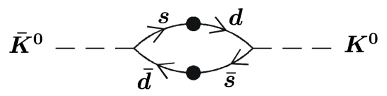
Figure 1: SOW $\bar{K}^{0}\leftrightarrow K^{0}$ SQL graph. Each dot represents the FOW SQL scale $\beta_{w}$.

as shown in Fig. 1. Combining Eq. (17) with Eq. (11), we find from data [4, 7]

$$\begin{array}[]{r}2\,\beta_{w}^{2}\;=\;\frac{\Delta m_{LS}}{m_{K}}\;=\;(0.70126\pm 0.00121)\times 10^{-14}\\ \Longrightarrow\;\;\;|\beta_{w}|\;\approx\;5.921\times 10^{-8}\;.\end{array}$$ (18)

Indeed, this FOW SQL scale $\beta_{w}$ (determined from the SOW $K_{L}\!-\!K_{S}$ mass difference) can be roughly estimated from the GIM $u\,,c$ self-energy graphs as [13, 14] $|\beta_{w}|\sim 5.6\times 10^{-8}$, not far from Eq. (18).

Substituting the FOW scale $\beta_{w}$ from Eq. (18) back into Eqs. (15) and (16) gives, for $f_{K}/f_{\pi}\approx 1.22$,

$$\left|M^{+-}_{K_{S}}\right|_{\mbox{\scriptsize$\Delta I\!=\!1/2$}}\;=\;2\,|\beta_{w}|\,\frac{f_{K}}{f^{2}_{\pi}}\,(m^{2}_{K}-m^{2}_{\pi})\;\approx\;35.5\times 10^{-8}\;\mbox{GeV}\;.$$ (19)

Also, the $\Delta I\!=\!3/2$ $W$-emission (WE) graph of Fig. 2 predicts

$$\!\!\!\!\!\!\left|\left<\pi^{+}\pi^{0}|H_{w}|K^{+}\right>\right|_{\mbox{\scriptsize WE}}=\left|\frac{G_{F}\,V_{ud}\,V_{su}}{2\sqrt{2}}\,(m^{2}_{K}\!-\!m^{2}_{\pi})\,f_{\pi}\right|\approx 1.86\times 10^{-8}\;\mbox{GeV}\;,$$ (20)

Figure 2: $\Delta I\!=\!3/2$ W-emission graph.

near data [4] $|M^{+0}_{K^{+}}|=(1.83\pm 0.01)\times 10^{-8}$ GeV. This WE amplitude, when extended to $K_{S}\!\to\!\pi^{+}\pi^{-}$, obviously doubles Eq. (20) to $2\times 1.86\approx 3.7\times 10^{-8}$ GeV. Then, the total $K_{S}\!\to\!\pi^{+}\pi^{-}$ amplitude is

$$\left|M^{+-}_{K_{S}}\right|_{\mbox{\scriptsize total}}\;=\;(35.5+3.7)\times 10^{-8}\;\mbox{GeV}\;=\;39.2\times 10^{-8}\;\mbox{GeV}\;,$$ (21)

very close to the measured amplitude for $q=206$ MeV [4], i.e.,

$$\left|M^{+-}_{K_{S}}\right|_{\mbox{\scriptsize PDG}}\;=\;m_{K}\,\sqrt{\frac{8\pi\Gamma^{+-}_{K_{S}}}{q}}\;=\;(39.1\pm 0.1)\times 10^{-8}\;\mbox{GeV}\;.$$ (22)

To test this SQL scale (18) in another way, we note that Eq. (16) predicts the FOW scale

$$\!\!\left|\left<\pi^{0}|H_{w}|K_{L}\right>\right|=\left|\left<\pi^{+}|H_{w}|K^{+}\right>\right|=2\,\beta_{w}\,m^{2}_{K}\,\frac{f_{K}}{f_{\pi}}\approx 3.58\times 10^{-8}\;\mbox{GeV}^{2}\;.$$ (23)

The latter scale is compatible with eleven data sets for $K_{S}\rightarrow 2\pi$, $K\rightarrow 3\pi$, $K_{L}\rightarrow 2\gamma$, $K_{L}\rightarrow\mu^{+}\mu^{-}$, $K^{+}\rightarrow\pi^{+}e^{+}e^{-}$, $K^{+}\rightarrow\pi^{+}\mu^{+}\mu^{-}$, and $\Omega^{-}\rightarrow\Xi^{0}\pi^{-}$, with data-average value [15]

$$\left|\left<\pi^{0}|H_{w}|K_{L}\right>\right|\;=\;\left|\left<\pi^{+}|H_{w}|K^{+}\right>\right|\;=\;(3.59\pm 0.05)\times 10^{-8}\;\mbox{GeV}^{2}\;.$$ (24)

In passing, we verify the $\Delta I\!=\!1/2$ rule via our theoretical estimate of the square of the amplitude in Eq. (21) relative to the one in Eq. (20):

$$\frac{|M^{+-}_{K_{S}}|\,^{2}}{|M^{+0}_{K^{+}}|\,^{2}}\;=\;\left(\frac{39.2\times 10^{-8}\;\mbox{GeV}}{1.86\times 10^{-8}\;\mbox{GeV}}\right)^{2}\;\approx\;444\;.$$ (25)

This is near the observed decay-rate ratio 450 found in Eq. (3).

6 Indirect and Direct CPV for $K\to 2\pi$ Decays

Now we study in detail indirect and direct CPV for $K_{2\pi}$ weak decays. Given that $|\eta_{+-}/\eta_{00}|$ is close to unity from data [4] in Eq. (7), years ago the leading term $|\varepsilon|$ was thought to be the $\alpha/\pi$ radiative correction

$$|\eta_{+-}|\;\approx\;|\eta_{00}|\;\approx\;|\varepsilon|\;\approx\;\frac{\alpha}{\pi}\;=\;2.32\times 10^{-3}\;,$$ (26)

as the origin of CPV [16, 8]. Actually, $\varepsilon^{\prime}$ cancels out in [4]

$$\varepsilon\;=\;\frac{2\eta_{+-}+\eta_{00}}{3}\;=\;(2.282\pm 0.017)\times 10^{-3}\;,$$ (27)

and this is the best measurement of the indirect CPV scale (yet still compatible with Eq. (26)). Concerning direct CPV, the ratio from Eq. (7) gives

$$\left|\frac{\eta_{+-}}{\eta_{00}}\right|\;\approx\;\frac{2.286\times 10^{-3}}{2.274\times 10^{-3}}\;\approx\;1.00528\;,$$ (28)

a close measure of unity. As a matter of fact, this direct CPV ratio should be [4]

$$\left|\frac{\eta_{+-}}{\eta_{00}}\right|\;\approx\;\left|\frac{\varepsilon+\varepsilon^{\prime}}{\varepsilon-2\varepsilon^{\prime}}\right|\;\approx\;1+3\,\frac{\varepsilon^{\prime}}{\varepsilon}\;.$$ (29)

Equating the CPV data ratio in Eq. (28) with the CPV theoretical ratio in Eq. (29) requires the direct CPV scale

$$\Re{\it e}\left(\frac{\varepsilon^{\prime}}{\varepsilon}\right)\;\approx\;17.6\times 10^{-4}\;.$$ (30)

The most recent direct CPV measurements for $K\to\pi\pi$ decays average to [3]

$$\Re{\it e}\left(\frac{\varepsilon^{\prime}}{\varepsilon}\right)\;=\;(16.6\pm 1.6)\times 10^{-4}$$ (31)

(this average includes the new NA48 result, and prior NA31, E731, and KTeV values). Note that Eq. (31) is near the approximate observed CPV scale in Eq. (30). In fact, the PDG/2002 quotes $\Re{\it e}\left(\varepsilon^{\prime}/\varepsilon\right)\;=\;(18\pm 4)\times 10^{-4}$.

The observed direct CPV is extracted from

$$\begin{array}[]{r}\displaystyle\Re{\it e}\left(\frac{\varepsilon^{\prime}}{\varepsilon}\right)\;=\;\frac{1}{6}\left(\frac{\Gamma_{K_{L}\to\pi^{+}\pi^{-}}\,/\,\Gamma_{K_{S}\to\pi^{+}\pi^{-}}}{\Gamma_{K_{L}\to\pi^{0}\pi^{0}}\,/\,\Gamma_{K_{S}\to\pi^{0}\pi^{0}}}\;-\;1\right)\\[11.38109pt] \displaystyle\Longrightarrow\;\;\;6\,\Re{\it e}\left(\frac{\varepsilon^{\prime}}{\varepsilon}\right)\;=\;\left(\frac{\eta_{+-}}{\eta_{00}}\right)^{2}\;-\;1\;.\end{array}$$ (32)

Substituting the latest direct CPV value (31) into Eq. (32) in turn gives

$$\left|\frac{\eta_{+-}}{\eta_{00}}\right|\;=\;1.00497\pm 0.00048\;,$$ (33)

and so a direct CPV scale enhancement of 0.497% does indeed hint at an e.m. correction to the FOW $K\to 2\pi$ amplitudes of Sec. 5, as we now demonstrate.

In quark-model $\Delta I\!=\!1/2$ SQL language, there are two different (see also below) radiatively corrected graphs to be considered for each charged final-state pion, as depicted in Fig. 3. Then the (direct) CPV (radiative)

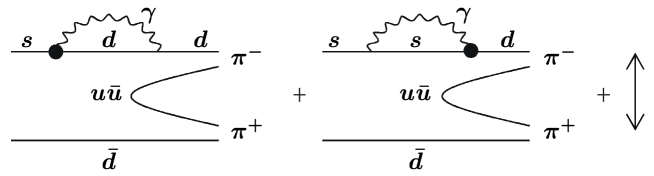
Figure 3: Radiatively corrected $\Delta I\!=\!1/2$ SQL graphs for $\bar{K}^{0}\to\pi^{+}\pi^{-}$.

amplitude ratio is predicted to be

$$\left|\frac{\eta_{+-}}{\eta_{00}}\right|_{\mbox{\scriptsize theory}}\;=\;1\,+\,2\,\frac{\alpha}{\pi}\;\approx\;1.00465\;,$$ (34)

and this 0.465% enhancement is very close to the 0.497% direct CPV enhancement in Eq. (33), and near the 0.528% approximate enhancement from Eq. (28) in the PDG tables.

First we comment on this crucial factor of 2 in Eq. (34). As a matter of fact, this was already discussed and explained in Ref. [24], having to do with the tadpole transition characterizing the $K\to 2\pi$ $\Delta I\!=\!1/2$ rule. Specifically, the $K^{0}$ $\bar{s}d$ meson (like the pion) is a tightly bound (relativistic) Nambu–Goldstone (NG) chiral meson. Then the “truly weak” tadpole ${\mathcal{O}}(m^{2}_{c}/M^{2}_{W})$ $\Delta I\!=\!1/2$ transition cannot be transformed away (as can be the loosely bound “purely e.m.” transition of ${\mathcal{O}}(\alpha^{2})$ [25]). Stated another way, the analog, now measured [26] $\kappa$(800) meson is generated in a unitarized coupled-channel approach [27], but cannot be found in a loosely bound (nonrelativistic) scheme. This means we must include the factor of 2 in Eq. (34) and Fig. 3, as these two photon-mediated loop graphs are distinct, since they both occur in NG (tightly bound) kaon configurations.

In the context of the SM, the only origin of CPV in the CKM scheme would be in the $3\times 3$ CKM matrix via the phase $\delta$, i.e. [note that we use here the original parametrization due to Kobayashi and Maskawa (Ref. [2], second paper; see also the PDG [4] CKM review), which is more convenient for our purposes],

$$V\;=\;\left(\begin{array}[]{ccc}V_{ud}&V_{us}&V_{ub}\\ V_{cd}&V_{cs}&V_{cb}\\ V_{td}&V_{ts}&V_{tb}\end{array}\right)\;=\;\left(\begin{array}[]{ccc}c_{1}&-s_{1}c_{3}&-s_{1}s_{3}\\ s_{1}c_{2}&c_{1}c_{2}c_{3}-s_{2}s_{3}e^{i\delta}&c_{1}c_{2}s_{3}+s_{2}c_{3}e^{i\delta}\\ s_{1}s_{2}&c_{1}s_{2}c_{3}+c_{2}s_{3}e^{i\delta}&c_{1}s_{2}s_{3}-c_{2}c_{3}e^{i\delta}\end{array}\right)$$ (35)

which can be written as

$$V\;\longrightarrow\;\left(\begin{array}[]{ccc}c_{1}&-s_{1}&0\\ s_{1}&c_{1}&0\\ 0&0&-(1+i\delta)\end{array}\right)$$ (36)

in the limit of an $SU(4)$ Cabibbo submatrix $\Theta_{1}=-\Theta_{c}$, and $\Theta_{2}\,,\Theta_{3}\to 0$. Then [8]

$$-V_{tb}\;=\;1+i\lambda_{w}\frac{\alpha}{\pi}\ln\left(1+\frac{\Lambda^{2}}{m_{t}^{2}}\right)$$ (37)

follows from the CKM tree and one-loop-order quark graphs of Fig. 4.

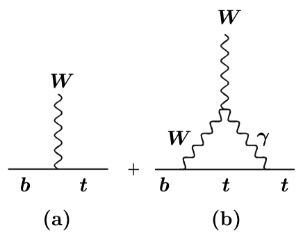
Figure 4: Tree-level (a) and loop-order (b) CKM element $V_{tb}$.

The CPV $WW\gamma\to V\!A\gamma$ vertex is defined as

$$\left<\gamma_{\mu}(q)W_{\beta}|W_{\alpha}\right>\;=\;ie\lambda_{w}\,\epsilon_{\alpha\beta\mu\sigma}\,q^{\sigma}\;,$$ (38)

then generating Eq. (37). The ultraviolet (chiral) cutoff is determined by the Veltman condition [18, 19], taking $m_{t}=174.3$ GeV [4] $>\!>m_{u},m_{d},m_{s},m_{c},m_{b}$, leading to

$$\Lambda^{2}\;=\;4m^{2}_{t}-(2M^{2}_{W}+M^{2}_{Z})\;\approx\;(316.7\;\mbox{GeV})^{2}\;.$$ (39)

Thus, Eq. (37) using the latter chiral cutoff in turn gives from Eq. (39) the phase

$$\delta\;=\;\lambda_{w}\frac{\alpha}{\pi}\ln 4.301\;=\;\lambda_{w}\,3.389\times 10^{-3}\;.$$ (40)

Comparing this CKM version of $\delta$ with the measurement of $\delta$ in Eq. (13), or with the theoretical estimate in Eq. (14), indeed suggests that the parameter $\lambda_{w}$ in the $V\!A\gamma$ CPV vertex (38) is unity. This parallels the standard e.m. minimal substitution $q_{\mu}\to q_{\mu}\!-\!eA_{\mu}$.

There are, however, various dynamical quark models characterizing the $V\!A\gamma$ CPV vertex. The Higgs exchange leading to a CPV neutron electric dipole moment (NEDM) $d_{n}$ suggested by Weinberg [20], giving $|d_{n}|\approx 4\times 10^{-24}\>e\!$ cm for $M_{H}\approx 316.7$ GeV, is ruled out by present data [4] finding $|d_{n}|<0.6\times 10^{-25}\>e\!$ cm, as noted by Pal & Pham [21]. An underlying NEDM version of the $WW\gamma$ CPV coupling has been often discussed in the literature [22]. Now that data appear to exclude a NEDM origin of CPV, we take the approximate equivalence between Eqs. (13), (14) and the CKM CPV Eq. (40) for $\lambda_{w}=1$ as the justification of a $V\!A\gamma$ vertex of unit strength, in a minimal-substitution sense. Here we should also note that a muon electric dipole moment (MEDM), now measured as [4] $d_{\mu}=(3.7\pm 3.4)\times 10^{-19}\>e\!$ cm, is not ruled out by our theory, which predicts $d_{\mu}=(4.2\times 10^{-21}\>e\,\mbox{cm})\,(m_{\mu}/2)\,\lambda_{w}\,\ln(1+\Lambda^{2}/M^{2}_{W})\,/\,1$ GeV $=\lambda_{w}\,0.62\times 10^{-21}\>e\!$ cm, for the same chiral cutoff $\Lambda=316.7$ GeV as in Eq. (39). If we then take $\lambda_{w}=1$, the latter MEDM prediction is clearly not excluded by experiment.

So whether we study the quark-model, photon-mediated graphs of Fig. 3 generating the CPV enhancement in $|\eta_{+-}/\eta_{00}|$ of 0.465%, or the CKM CPV phase $\delta\approx(3.3\,$–$\,3.4)\times 10^{-3}$ generated via the $WW\gamma$ triangle enhancement of Fig. 4, CPV for $K\to 2\pi$ decays appears to follow from photon-mediated loop enhancement. Alternatively, one may compute the small imaginary corrections to the amplitude for $K^{0}$-$\bar{K}^{0}$ transitions, employing the standard double-$W$ box diagrams, but accounting for the physical decay thresholds of the $W$ and sandwiching the whole amplitude between composite-kaon vertex functions, which results in an effect surprisingly close to the value of $|\varepsilon|$ [23]. However, the latter $WW$-box result is the same as the indirect CPV value in the present SQL $K^{0}$-$\bar{K^{0}}$ scheme of Fig. 1 and Eqs. (17,18).

Another weak-interaction radiative correction of this small size follows from the semileptonic weak $\mu^{-}\to e^{-}\nu_{\mu}\bar{\nu}_{e}$ decay. Long ago, Kinoshita & Sirlin [28] computed this net $V\!-\!A$ rate correction due to radiative effects as

$$\frac{\Gamma-\Gamma_{0}}{\Gamma_{0}}\;=\;\frac{\alpha}{2\pi}\,\left(\pi^{2}-\frac{25}{4}\right)\;\approx\;0.42\,\%\;.$$ (41)

We note that this 0.42% radiative enhancement is near the 0.465% e.m. enhancement for $K\to 2\pi$, or the observed direct CPV scale of 0.497%.

7 Summary and Conclusions

In the foregoing, we have analyzed remarkable patterns in the experimental data for CPC and CPV $K\to 2\pi$ and $K\to 2\pi\gamma$ weak decays, as well as for $\Delta I\!=\!1/2$ compared to $\Delta I\!=\!3/2$ processes. Concretely, in Sec. 2 we extracted from data [4] the 4.5% to 4.7% $\Delta I\!=\!3/2$ suppression in both CPC and CPV $K\to 2\pi$ transitions. Next, in Sec. 3 we found that the observed $K\to\pi\pi\gamma/\pi\pi$ branching ratios are all scaled near $\alpha/\pi$ or $\alpha/2\pi$. Then in Sec. 4 we studied the CPV angles $\phi$ and $\delta$. In Sec. 5 we returned to $K\to 2\pi$ $\Delta I\!=\!1/2$ dominance from the perspective of the chiral (constituent) quark model. Finally, in Sec. 6 we studied indirect and direct kaon CPV in the framework of photon-mediated loop graphs via 0.497%, 0.465%, 0.42% values, obtained from direct CPV data, and theoretical radiatively corrected $K\to 2\pi$ and $\mu\to e\nu\bar{\nu}$ weak amplitudes.

We have not considered strong-interaction penguin graphs in our analysis, as the typical QCD scale of $\sim$ 1 fm is orders of magnitude larger than the electroweak CPV scale of about $0.0023\times 1/M_{W}=5.6\times 10^{-6}$ fm. Therefore, we argue it is unlikely that such graphs yield a significant contribution to CPV-related processes. This qualitative argument is confirmed by explicit calculations, showing that QCD penguins lead to much too small results for $\Delta I\!=\!1/2$ nonleptonic kaon decay rates [29], as well as for the CPV ratio $\epsilon^{\prime}/\epsilon$ [30]. Also Lucio [31] showed, using inner-bremsstrahlung and direct-emission graphs, that QCD penguins do not play an important role in $\Delta I\!=\!1/2$ $\,K\to\pi\pi\gamma$ transitions.

Summarizing, we have shown that CPV — at least for kaon weak decays involving two pions — can be described with standard second-order weak physics, radiatively corrected. We believe this line of research should be further pursued for other CPV processes, too, as a possible alternative to new physics.

To conclude, we present CPV to CPC decay-rate ratios for various PDG [4] kaon-decay processes involving two pions, as extra support for our analysis:

$$\frac{\Gamma_{K_{L}\,\to\,\pi^{+}\pi^{-}}}{\Gamma_{K_{S}\,\to\,\pi^{+}\pi^{-}}}\;\; = \;\;(5.25\pm 0.12)\times 10^{-6}\;,$$ (42)

$$\mbox{close to}\;\;\;|\eta_{+-}|^{2}\;\; = \;\;(5.23\pm 0.08)\times 10^{-6}\;;$$ (43)

$$\frac{\Gamma_{K_{L}\,\to\,\pi^{0}\pi^{0}}}{\Gamma_{K_{S}\,\to\,\pi^{0}\pi^{0}}}\;\; = \;\;(5.19\pm 0.20)\times 10^{-6}\;,$$ (44)

$$\mbox{close to}\;\;\;|\eta_{00}|^{2}\;\; = \;\;(5.17\pm 0.08)\times 10^{-6}\;;$$ (45)

$$\frac{\Gamma_{K_{L}\,\to\,\pi^{+}\pi^{-}e^{+}e^{-}}}{\Gamma_{K_{S}\,\to\,\pi^{+}\pi^{-}e^{+}e^{-}}}\;\; = \;\;(13.4\pm 3.3)\times 10^{-6}\;;$$ (46)

$$\frac{\left(\Gamma_{K_{L}\,\to\,\pi^{+}\pi^{-}\gamma}\right)_{\mbox{\scriptsize CPV}}}{\Gamma_{K_{S}\,\to\,\pi^{+}\pi^{-}\gamma}}\;\; = \;\;|\eta_{+-\gamma}|^{2}\;\;=\;\;(5.52\pm 0.33)\times 10^{-6}\;.$$ (47)

Note that the experimental rate ratio in Eq. (46) has a large error, suggesting that it might also turn out to be close to the average value of $(5.2\pm 0.1)\times 10^{-6}$ in Eqs. (42)–(47), being about 2.5 standard deviations away. Finally, as the CPV component of the process $K_{L}\to\pi^{+}\pi^{-}\gamma$ is not yet known experimentally, we have used in Eq. (47) the equality of the corresponding rate ratio with the measured quantity $|\eta_{+-\gamma}|^{2}$. Clearly, more and still better experiments, also in the kaon sector, are needed to lend additional evidence to our interpretation of CPV as a radiatively corrected SOW effect.

Acknowledgments
We wish to thank F. Kleefeld for valuable discussions. This work was partly supported by the Fundação para a Ciência e a Tecnologia of the Ministério da Ciência e do Ensino Superior of Portugal, under contract no. POCTI/FNU/49555/2002.

References

- [1] J. H. Christenson, J. W. Cronin, V. L. Fitch, and R. Turlay, Phys. Rev. Lett. 13, 138 (1964).
- [2] N. Cabibbo, Phys. Rev. Lett. 10, 531 (1963); M. Kobayashi and T. Maskawa, Prog. Theor. Phys. 49, 652 (1973).
- [3] Y. Nir, Nucl. Phys. Proc. Suppl. 117, 111 (2003).
- [4] K. Hagiwara et al. [Particle Data Group Collaboration], Phys. Rev. D66, 010001 (2002).
- [5] L. B. Okun, Leptons and Quarks, North-Holland Physics Publishing, Amsterdam (1982,1984), ISBN 0444860029; see pp. 77–79.
- [6] B. de Wit and J. Smith, Field Theory In Particle Physics, Vol. 1, North-Holland Physics Publishing, Amsterdam (1986), ISBN 0444869964; see pp. 157–162.
- [7] M. D. Scadron and V. Elias, Mod. Phys. Lett. A10, 1159 (1995).
- [8] S. R. Choudhury and M. D. Scadron, Phys. Rev. D53, 2421 (1996).
- [9] See e.g. R. E. Marshak, Riazuddin, and C. P. Ryan, Theory of Weak Interactions in Particle Physics, Wiley-Interscience, NY (1969), page 641.
- [10] R. E. Karlsen and M. D. Scadron, Phys. Rev. D45, 4108 (1992).
- [11] R. E. Karlsen and M. D. Scadron, Nuovo Cim. A106, 237 (1993).
- [12] J. A. Cronin, Phys. Rev. 161, 1483 (1967); also see R. E. Karlsen and M. D. Scadron, Mod. Phys. Lett. A10, 1247 (1995).
- [13] S. L. Glashow, J. Iliopoulos, and L. Maiani, Phys. Rev. D2, 1285 (1970).
- [14] M. D. Scadron, Rept. Prog. Phys. 44, 213 (1981); R. Delbourgo and M. D. Scadron, Lett. Nuovo Cim. 44, 193 (1985).
- [15] J. Lowe and M. D. Scadron, Mod. Phys. Lett. A17, 2497 (2002).
- [16] J. Bernstein, G. Feinberg, and T. D. Lee, Phys. Rev. 139, B1650 (1965); S. Barshay, Phys. Lett. 17, 78 (1965); A. Arbugon and A. T. Fillipov, Phys. Lett. 20, 537 (1966); W. J. Marciano and A. Queijeiro, Phys. Rev. D33, 3449 (1986). The latter authors are skeptical concerning an analog (but as yet unmeasured) neutron electric dipole moment.
- [17] J. F. Donoghue, E. Golowich, and B. R. Holstein, Dynamics Of The Standard Model, Cambridge University Press (1994), ISBN 0521476526; see page 241.
- [18] M. J. Veltman, Acta Phys. Polon. B12, 437 (1981).
- [19] The weak chiral NJL analog GeV, for [4] GeV, was originally interpreted as the squared Higgs mass by a number of authors: Y. Nambu, Proc. Workshop Dynamical symmetry breaking, 21–23 Dec 1989, Nagoya, Japan, pp. 1–10; M. D. Scadron, Phys. Atom. Nucl. 56, 1595 (1993) [Yad. Fiz. 56N11, 245 (1993)]; G. Lopez Castro and J. Pestieau, Mod. Phys. Lett. A10, 1155 (1995).
- [20] S. Weinberg, Phys. Rev. Lett. 37, 657 (1976).
- [21] P. B. Pal and T. N. Pham, Z. Phys. C47, 663 (1990).
- [22] F. Salzman and G. Salzman, Phys. Lett. 15, 91 (1965); Nuovo Cim. A41, 443 (1966); S. Weinberg, Ref. [20] above; N. G. Deshpande, G. Eilam, and W. L. Spence, Phys. Lett. B108, 42 (1982); P. B. Pal and T. N. Pham, Ref. [21] above; W. J. Marciano and A. Queijeiro, in Ref. [16] above; T. P. Cheng and L. F. Li, Phys. Lett. B234, 165 (1990).
- [23] Eef van Beveren and George Rupp, hep-ph/0308030.
- [24] B. H. McKellar and M. D. Scadron, Phys. Rev. D27, 157 (1983).
- [25] S. Weinberg, Phys. Rev. Lett. 31, 494 (1973); Phys. Rev. D8, 605 (1973).
- [26] E. M. Aitala et al. [E791 Collaboration], Phys. Rev. Lett. 89, 121801 (2002).
- [27] E. van Beveren, T. A. Rijken, K. Metzger, C. Dullemond, G. Rupp, and J. E. Ribeiro, Z. Phys. C30, 615 (1986).
- [28] T. Kinoshita and A. Sirlin, Phys. Rev. 113, 1652 (1959); see Eq. (2.13); A. Sirlin, Rev. Mod. Phys. 50, 573 (1978) [Erratum-ibid. 50, 905 (1978)].
- [29] R. S. Chivukula, J. M. Flynn, and H. Georgi, Phys. Lett. B171, 453 (1986); also see C. T. Hill and G. G. Ross, Phys. Lett. B94, 234 (1980).
- [30] A. J. Buras, Proc. Conf. Kaon Physics (K 99), 21–26 Jun 1999, Chicago, IL, pp. 67–87, hep-ph/9908395. The author finds that the CPV gluonic penguin graph generates only about 10% of the KTeV value. See also A. J. Buras, M. Jamin, and M. E. Lautenbacher, Nucl. Phys. B408, 209 (1993); A. J. Buras, Acta Phys. Polon. B26, 755 (1995).
- [31] J. L. Lucio, Phys. Rev. D24, 2457 (1981).