Out-of-equilibrium electromagnetic radiation

Abstract:

We derive general formulas for photon and dilepton production rates from an arbitrary non-equilibrated medium from first principles in quantum field theory. At lowest order in the electromagnetic coupling constant, these relate the rates to the unequal-time in-medium photon polarization tensor and generalize the corresponding expressions for a system in thermodynamic equilibrium. We formulate the question of electromagnetic radiation in real time as an initial value problem and consistently describe the virtual electromagnetic dressing of the initial state. In the limit of slowly evolving systems, we recover known expressions for the emission rates and work out the first correction to the static formulas in a systematic gradient expansion. Finally, we discuss the possible application of recently developed techniques in non-equilibrium quantum field theory to the problem of electromagnetic radiation. We argue, in particular, that the two-particle-irreducible (2PI) effective action formalism provides a powerful resummation scheme for the description of multiple scattering effects, such as the Landau-Pomeranchuk-Migdal suppression recently discussed in the context of equilibrium QCD.

1 Introduction

1.1 Motivations and overview of previous works

Because they interact weakly with matter, direct electromagnetic signals provide sensitive probes of the hot and dense matter produced in high energy heavy ion collisions [1]. Once emitted, they mostly escape the collision zone without further interaction and, therefore, carry direct information about the state of the emitting system at the various stages of its time evolution. Recently, the WA98 collaboration has reported the first observation of direct photons in central $Pb$–$Pb$ collisions at the CERN SPS [2]. The measurement of direct photons and dileptons is one of the major goals of the PHENIX experiment at RHIC [3] and is among the key observables to be studied by the ALICE collaboration at the LHC [4].

Electromagnetic probes are expected to be directly sensitive to the (partonic or hadronic) nature of the relevant degrees of freedom underlying the dynamics of the produced matter. They have been proposed as a promising signature of the possible formation of a deconfined state of matter, the so-called quark-gluon plasma [5, 6]. An intense theoretical activity has been devoted to study the emissive power of a quark-gluon plasma vs. that of a hot hadron gas in thermodynamic equilibrium (for recent reviews see [7, 8]). Both are highly non-trivial problems, which require, in particular, a detailed understanding of various medium effects such as, for instance in the former case, dynamical screening [9, 10], or interference effects between multiple scattering processes, the so-called Landau-Pomeranchuk-Migdal effect [11, 12, 13] (for a recent short review, see [14]). To make contact with phenomenology, one has to model the space-time evolution of the fireball. For this purpose, one usually makes the simplifying assumption that, due to their multiple interactions, the produced partons thermalize (locally) shortly after the initial impact. The integration over space-time is then performed by folding the equilibrium rates, computed in either the deconfined or the hadronic phase, with a given hydrodynamic model (see e.g. [15]), which includes, in particular, a modelization of the equation of state in both phases as well as of the phase transition (for a recent review, see [16]).

However, although ideal hydrodynamics is doing remarkably well in describing data such as elliptic flow or transverse spectra at not too high momenta [17], the assumption of early thermalization appears questionable, at least from the point of view of perturbative QCD (see e.g. [18]). Indeed, detailed theoretical studies of the early-time evolution of the partonic system reveal that the so-called pre-equilibrium stage may not be as short as usually believed. In particular, in very energetic collisions at RHIC and at LHC, where it is expected that the partons produced in the central rapidity region are mostly gluons, it appears that elementary QCD processes are not fast enough to lead to efficient chemical equilibration between gluon and (anti-)quark populations [19]. Moreover, recent studies of kinetic equilibration have shown that it is extremely difficult to reach thermal equilibrium on time scales lower than a few fm/c, due to the strong longitudinal expansion at very early times [20]. Although the issue of early thermalization is still a matter of debate (see e.g. [21]), it seems important to consider the influence of the non-equilibrium evolution on the various experimental signatures of the produced matter and, in particular, on electromagnetic signals, which are sensitive to the earliest stages of the collision.

There are various other motivations for studying out-of-equilibrium electromagnetic radiation in the context of heavy ion collisions. For instance, it is expected that a non-trivial semi-classical pion field configuration might form during the rapid cooling of the system through the chiral phase transition [22]. The electromagnetic radiation associated with the decay of this so-called disoriented chiral condensate has been proposed as a possible signature of the phenomenon [23, 24], which in turn might provide a useful tool to locate the critical point of the QCD phase diagram [25]. Another interesting motivation is related to the fact that, because of their sensitivity to the early stages of the collision, direct electromagnetic signals might bring experimental information concerning the initial conditions realized after the nuclear impact.

Various aspects of out-of-equilibrium electromagnetic radiation have been addressed in the literature, in particular in the context of an under-saturated partonic plasma, where local kinetic equilibrium is assumed to be rapidly achieved, but where quarks and gluons are not yet chemically equilibrated [26, 27, 28]. In that case, the momentum distributions of quarks and gluons are isotropic and one can closely follow equilibrium calculations. In particular, one can generalize the so-called hard thermal loop (HTL) resummation and extend the usual analysis of dynamical screening to the non-equilibrium case [28]. So far, these calculations have been pushed up to the two-loop level [29] and lead to significantly different results from the corresponding equilibrium calculations because of the low population of quarks and anti-quarks at early times [30, 29]. The case of a system out of kinetic equilibrium has been much less studied. Attempts in this direction generally rely on folding general distribution functions, taken to be the solutions of appropriate Boltzmann equations, with conventional matrix elements [31, 32]. This, however, does not provide a consistent description of phenomena like screening and one generally has to introduce an infra-red cut-off by hand. Although one can also formulate the analog of the HTL resummation in that case (see e.g. [33]), it is more difficult to employ in practice because momentum integrations cannot be explicitly performed for arbitrary distribution functions.

An important remark to be done concerning the above calculations is that, unlike their equilibrium counterpart, they do not rely on a first principle derivation of the out-of-equilibrium photon and dilepton production rates. For instance, the most widely used ansatz is to start with equilibrium-like expressions for the rates, written at a given space-time point, and to simply replace the Bose-Einstein and Fermi-Dirac distribution functions appearing e.g. in the real-time equilibrium formalism by other functions of momentum reflecting the out-of-equilibrium particle distribution in phase-space. This procedure would be exact for general stationary systems; it might also be justified when the duration of the emission process is short enough as compared to the typical relaxation time of the emitting system [34]; but it can clearly not be universally valid for computing non-equilibrium processes. In the general case, one expects the emission process to depend non-locally on the space-time history of the emitting system and the main issue is to properly formulate the production rate itself. An attempt in this direction has been made in Ref. [35]. However, the approach presented there is widely based on the use of standard perturbation theory, which is known to be badly suited for the description of non-equilibrium systems. Interesting steps towards a more satisfying formulation of the problem have been made recently in a slightly different context in Refs. [42, 43, 44], where the authors discuss possible finite lifetime effects for a system in equilibrium. Still, the real-time formulation of [42] suffers from serious physical problems such as spontaneous photon emission from the vaccum or infinite amounts of radiated energy [43]. These difficulties can be traced back to the issue of properly identifying and subtracting the unobservable virtual radiation at any finite time [44].

1.2 Summary of the present work

In this paper, we address the question of out-of-equilibrium electromagnetic radiation from a very general point of view and present a first principle derivation of photon and dilepton emission rates in the framework of non-equilibrium quantum field theory. We treat electromagnetic interactions at lowest order in perturbation theory but, otherwise, make no assumption concerning the internal dynamics of the emitting system. Our approach generalizes the real-time formulation of Boyanovsky et al. [42] to the case of arbitrarily far-from-equilibrium systems. In order to deal with the problem of virtual radiation mentioned above, we propose to consistently take into account the electromagnetic dressing of the initial state. In particular, this allows one to unambiguously identify the virtual contribution at the initial time and to subtract it at once.

We obtain general formulas relating the out-of-equilibrium production rates to the intrinsic dynamics of the emitting system which, at lowest order in the electromagnetic coupling constant, is characterized by the non-equilibrium in-medium photon polarization tensor. This generalizes the corresponding formulas in equilibrium [1, 45, 46], which we recover in the appropriate limit. In particular, we show that the description of the initial virtual cloud is essential in order to recover known formulas for the particular case of stationary systems. We also discuss the case of slowly evolving (quasi-stationary) systems and derive the first corrections to the static photon and dilepton production rates in a standard gradient expansion.

In the last part of the paper, we make contact with recent progress concerning the description of far-from-equilibrium quantum fields, based e.g. on the so-called two-particle-irreducible (2PI) effective action formalism [47], or on truncations of Schwinger-Dyson equations [48] (for a recent review, see [49]). In particular, these methods allow for practical, first principle calculations of the non-equilibrium dynamics in realistic particle physics applications [50, 51]. We discuss how they might be employed in the present context and propose a formalism, based on introducing a ${\cal S}$–shape path in real time, which allows one to generalize existing methods to the case of dressed initial states. Finally, we outline how the relevant current-current correlator can be obtained within the 2PI effective action formalism. We point out that finite order approximations of the 2PI effective action automatically generates infinite resumations of ladder-type diagrams, which correspond to multiple scattering processes. Recall that the latter have recently been shown to play a crucial role in obtaining the full photon and dilepton production rates from an equilibrated QCD plasma at leading order in $\alpha_{s}$ [12, 13].

2 The non-equilibrium set-up

We consider a system of interacting (bosonic and/or fermionic) fields, prepared in a given out-of-equilibrium initial state, and which emits photons and lepton pairs in the course of its time evolution. We assume that the relative energy loss is negligible so that the process of electromagnetic emission can be considered as a small perturbation. Our aim in this section is to relate, at lowest order in perturbation theory, the inclusive spectrum of radiated photons and lepton pairs to the intrinsic non-equilibrium dynamics of the emitting system, without further approximations.

2.1 Initial value problem: Schwinger’s closed time-path

We denote by $H_{\rm s}$ the Hamiltonian describing the internal dynamics of the emitting system which we assume has been prepared at time $t=0$ in an arbitrary state characterized by the (normalized) density matrix $\rho_{\rm s}$. In terms of the eigenstates $|n,{\rm s}\rangle$ of $H_{\rm s}$, where $n$ denotes a set of relevant quantum numbers, the latter can be written

$$\rho_{\rm s}=\sum_{n,m}P^{\rm s}_{nm}\,|n,{\rm s}\rangle\langle m,{\rm s}|\,,$$ (1)

with $P^{\rm s}_{nm}\equiv\langle n,{\rm s}|\rho_{\rm s}|m,{\rm s}\rangle$. Similarly, we denote by $H_{\rm em}$ the Hamiltonian describing free propagation of electromagnetic degrees of freedom, that is photons and (anti-)leptons, and by $\rho_{\rm em}$ the density matrix characterizing the initial state of the electromagnetic sector. As above, one can write:

$$\rho_{\rm em}=\sum_{a,b}P^{\rm em}_{ab}\,|a,{\rm em}\rangle\langle b,{\rm em}|$$ (2)

in terms of the eigenstates $|a,{\rm em}\rangle$ of $H_{\rm em}$.

In absence of electromagnetic interactions, the most general density matrix for the whole system ‘emitter+radiation’ has the factorized form:

$$\bar{\rho}=\rho_{\rm s}\otimes\rho_{\rm em}\,.$$ (3)

At this order of approximation, the two subsystems evolve independently: The time-evolution of the emitter is driven by the interactions between its internal degrees of freedom, whereas the (free) electromagnetic sector undergo a trivial evolution from the initial state (2). Introducing electromagnetic interactions, the total Hamiltonian reads:

$$H=H_{\rm s}+H_{\rm em}+H_{\rm int}\,,$$ (4)

where $H_{\rm int}$ represents the coupling of the photon field with the degrees of freedom of the emitting system as well as with leptons. In general, electromagnetic interactions might also introduce non-trivial correlations between the emitting system and the electromagnetic degrees of freedom in the initial state and the total density matrix $\rho$ cannot be factorized as in Eq. (3). As mentioned in the introduction, we are interested in describing the virtual electromagnetic cloud associated with the charged degrees of freedom of the emitting system. The corresponding density matrix can be formally obtained by “dressing” the bare initial state (3): The dressed states $|n,a\rangle$ can be expressed in terms of the unperturbed states as follows (up to an overall phase) [52] (see also [44]):

$$|n,a\rangle=U_{\epsilon}(0,-\infty)\,|n,{\rm s}\rangle\otimes|a,{\rm em}\rangle\,,$$ (5)

where the unitary “dressing” operator $U_{\epsilon}(0,-\infty)$ is formally equivalent to an adiabatic switching-on of electromagnetic interactions from the infinite past:

$$U_{\epsilon}(0,-\infty)={\rm T}\exp\Big{\{}-i\int_{-\infty}^{0}du\,{\rm e}^{\epsilon u}\,H_{\rm I}(u)\Big{\}}=U^{\dagger}_{\epsilon}(-\infty,0)\,.$$ (6)

with $\epsilon\equiv 0^{+}$.

$$H_{\rm I}(t)={\rm e}^{i(H_{\rm s}+H_{\rm em})t}\,H_{\rm int}\,{\rm e}^{-i(H_{\rm s}+H_{\rm em})t}\,.$$ (7)

Using Eqs. (1)-(3) and (5), one obtains the required dressed density matrix, in terms of the bare one:

$$\rho=U_{\epsilon}(0,-\infty)\,\bar{\rho}\,U_{\epsilon}^{\dagger}(0,-\infty)\,.$$ (8)

Once the initial state has been specified, the subsequent non-equilibrium evolution is completely determined by the full Hamiltonian $H$. We shall typically be interested in unequal-time correlation functions of the form:

$$\langle{\cal O}(t_{1})\cdots{\cal O}(t_{n})\rangle\equiv{\rm Tr}[\,\rho\,{\cal O}(t_{1})\cdots{\cal O}(t_{n})]\,,$$ (9)

where the time evolution of a given operator ${\cal O}$ is given by

$${\cal O}(t)={\rm e}^{iH\,t}\,{\cal O}\,{\rm e}^{-iH\,t}\,.$$ (10)

For given initial conditions, specified at $t=0$ and characterized by the density matrix $\rho$, the above correlation functions may be computed by introducing a finite closed path in real time [53], as shown in Fig. 1.

Figure 1: The Schwinger closed time path. In this formulation, the initial condition is specified at the initial time $t=0$ and is characterized by the dressed density matrix $\rho$.

2.2 Virtual cloud vs. virtual time evolution: revisiting Keldysh’s time-path

In this subsection, we exploit the preceeding adiabatic construction, in order to replace the initial correlations due to electromagnetic dressing by a formally equivalent time evolution from an uncorrelated state of the form (3) in the infinite past. This allows us to treat the virtual dressing of the initial state and the process of radiation during the physical time evolution on a similar footing and considerably simplifies the calculations.

To make this more precise, we make use of the interaction picture with respect to the unperturbed Hamiltonian $H_{\rm s}+H_{\rm em}$ introduced above:

$${\cal O}_{\rm I}(t)={\rm e}^{i(H_{\rm s}+H_{\rm em})t}\,{\cal O}\,{\rm e}^{-i(H_{\rm s}+H_{\rm em})t}\,.$$ (11)

Interaction picture operators are related to Heisenberg operators via:

$${\cal O}(t)=U^{\dagger}(t,0)\,{\cal O}_{I}(t)\,U(t,0)\,,$$ (12)

where

$$U(t,t^{\prime})={\rm T}\exp\Big{\{}-i\int_{t^{\prime}}^{t}du\,H_{\rm I}(u)\Big{\}}=U^{\dagger}(t^{\prime},t)\,.$$ (13)

For the sake of the argument, we focus here on the case of a two-point correlation function. The generalization to higher correlation functions is straightforward. Using the form (8) of the density matrix and noticing that

$${\rm Tr}[\rho]={\rm Tr}[\bar{\rho}]=1\,,$$ (14)

we can write ($t>t^{\prime}\geq 0$):

$$\langle{\cal O}(t)\,{\cal O}(t^{\prime})\rangle = {\rm Tr}\Big{[}\,\rho\,\,U(0,t)\,{\cal O}_{\rm I}(t)\,U(t,t^{\prime})\,{\cal O}_{\rm I}(t^{\prime})\,U(t^{\prime},0)\Big{]}$$ (15)

$$= {\rm Tr}\Big{[}\,\bar{\rho}\,\,U_{\epsilon}(-\infty,0)\,U(0,t)\,{\cal O}_{\rm I}(t)\,U(t,0)\,U_{\epsilon}(0,-\infty)$$

$$\quad\times U_{\epsilon}(-\infty,0)\,U(0,t^{\prime})\,{\cal O}_{\rm I}(t^{\prime})\,U(t^{\prime},0)\,U_{\epsilon}(0,-\infty)\Big{]}$$

$$= {\rm Tr}\Big{[}\,\bar{\rho}\,\,V_{\epsilon}(-\infty,t)\,{\cal O}_{\rm I}(t)\,V_{\epsilon}(t,t^{\prime})\,{\cal O}_{\rm I}(t^{\prime})\,V_{\epsilon}(t^{\prime},-\infty)\Big{]}\,,$$

where we defined the unitary operator

$$V_{\epsilon}(t,t^{\prime})={\rm T}\exp\Big{(}-i\int_{t^{\prime}}^{t}[du]\,H_{\rm I}(u)\Big{)}=V^{\dagger}_{\epsilon}(t^{\prime},t)\,,$$ (16)

which satisfies the relation:

$$V_{\epsilon}(t,-\infty)=U(t,0)\,U_{\epsilon}(0,-\infty)\,.$$ (17)

Here, we introduced the shorthand notation:

$$[du]\equiv du\,[\,\theta(-u)\,{\rm e}^{\epsilon u}+\theta(u)\,]\,.$$ (18)

Reading the first line of Eq. (15) from right to left, one clearly sees the time evolution from $t=0$ to the positive time $t^{\prime}$, then to $t>t^{\prime}$ and, finally, back to $t=0$. This is the essence of the closed time path formulation corresponding to the contour of Fig. 1. Here, the initial state is specified at $t=0$ and is characterized by the dressed density matrix $\rho$. Similarly, we clearly see, from the third line of Eq. (15), that this can be reformulated as a “time-evolution” along the contour of Fig. 2, which extend to the infinite past, and where the “initial” state, now specified at $t=-\infty$, is characterized by the bare density matrix $\bar{\rho}$. The closed path ${\cal C}$ along the real axis, represented on Fig. 2, is sometimes referred to as the Keldysh contour [54] in the literature. It is useful to introduce time-ordered correlation functions along the contour, which can be written as (see Eq. (15)):

$$\Big{<}T_{\cal C}\Big{\{}{\cal O}(t_{1})\cdots{\cal O}(t_{n})\Big{\}}\Big{>}={\rm Tr}\left[\,\bar{\rho}\,\,T_{\cal C}\Big{\{}{\cal O}_{\rm I}(t_{1})\cdots{\cal O}_{\rm I}(t_{n})\,\exp\Big{(}-i\int_{\cal C}[du]\,H_{\rm I}(u)\Big{)}\Big{\}}\right]\,,$$ (19)

where $T_{\cal C}$ represents time-ordering along ${\cal C}$. We mention that one can equivalently formulate the above construction in terms of path integrals by means of standard manipulations (see also section 5 below).

Figure 2: The electromagnetic dressing of the initial state at time $t=0$ is formally equivalent to a time evolution from a state characterized by the bare density matrix $\bar{\rho}$ at $t=-\infty$ to the physical initial time $t=0$. This can be described by introducing the above (Keldysh) path in real time.

In the following, we shall use standard notations for two-point correlation functions:

$${\rm C}_{\alpha\beta}(t,t^{\prime}) \equiv \Big{<}{\rm T}_{\cal C}\Big{\{}{\cal O}_{\alpha}(t)\,{\cal O}_{\beta}(t^{\prime})\Big{\}}\Big{>}$$ (20)

$$= \Theta_{\cal C}(t-t^{\prime})\,{\rm C}^{>}_{\alpha\beta}(t,t^{\prime})\pm\Theta_{\cal C}(t^{\prime}-t)\,{\rm C}^{<}_{\alpha\beta}(t,t^{\prime})\,,$$

where ${\cal O}_{\alpha}$ and ${\cal O}_{\beta}$ are two arbitrary operators and $\alpha$ and $\beta$ represent a set of (Dirac, Lorentz, etc …) indices and/or spatial variables. The plus/minus sign corresponds to the case of bosonic/fermionic operators respectively and the the two independent components are given by:

$${\rm C}^{>}_{\alpha\beta}(t,t^{\prime}) = \langle{\cal O}_{\alpha}(t)\,{\cal O}_{\beta}(t^{\prime})\rangle\,,$$ (21)

$${\rm C}^{<}_{\alpha\beta}(t,t^{\prime}) = \langle{\cal O}_{\beta}(t^{\prime})\,{\cal O}_{\alpha}(t)\rangle\,.$$ (22)

3 Out-of-equilibrium electromagnetic radiation

We now apply the formalism described above to the calculation of the out-of-equilibrium photon and dilepton production rates as a function of time, at leading order in the electromagnetic coupling constant. Assuming that no real electromagnetic radiation is present initially, the initial state is described by Eqs. (3) and (8) with

$$\rho_{\rm em}=|0,{\rm em}\rangle\langle 0,{\rm em}|\,.$$ (23)

The generalization of the following considerations to the case where real radiation is already present in the initial state is straightforward. Note that the density matrix $\rho_{\rm s}$ describing the initial state of the emitting system is left arbitrary. We assume that the electromagnetic interaction Hamiltonian has the following form (in the Schrödinger picture):

$$H_{\rm int}=\int d^{3}x\,{\cal J}^{\mu}({\vec{x}})\,A_{\mu}({\vec{x}})\,,$$ (24)

where $A^{\mu}({\vec{x}})$ is the electromagnetic field operator and

$${\cal J}^{\mu}({\vec{x}})=J^{\mu}({\vec{x}})+j^{\mu}({\vec{x}})$$ (25)

is the total electromagnetic current, including the contributions from both the emitting system ($J^{\mu}$) and the leptonic fields $\psi$:

$$j^{\mu}({\vec{x}})=e\,\bar{\psi}({\vec{x}})\gamma^{\mu}\psi({\vec{x}})\,.$$ (26)

Here, $e$ denotes the electromagnetic coupling constant and $\gamma^{\mu}$ are the usual Dirac matrices. In the case where the emitting system contains charged scalar fields, there is an additional contribution – quadratic in the photon field – to the interaction Hamiltonian (24). We shall consider such a term at the end of this section. From now on, we specialize to the case of spatially homogeneous systems for simplicity.

3.1 Inclusive photon spectrum at time $t$

At a given time $t$, the single-particle inclusive photon spectrum can be expressed as:

$$\frac{dn_{\gamma}(t,{\vec{k}})}{d^{3}x\,d^{3}k}=\frac{1}{(2\pi)^{3}}\,\sum_{\lambda=\perp}\Big{<}N^{(\lambda)}_{\gamma}(t,{\vec{k}})\Big{>}\,,$$ (27)

where the sum runs over physical (transverse) polarizations. Here,

$$N^{(\lambda)}_{\gamma}(t,{\vec{k}})\equiv a_{\lambda}^{\dagger}(t,{\vec{k}})\,a_{\lambda}(t,{\vec{k}})$$ (28)

denotes the Heisenberg picture of the photon number operator for momentum ${\vec{k}}$ and polarization $\lambda$. The corresponding creation and annihilation operators are related to the electromagnetic field operator and its time derivative through:

$$a_{\lambda}(t,{\vec{k}})=-\frac{\epsilon^{(\lambda)}({\vec{k}})}{\sqrt{2k}}\cdot\Big{[}i\,\dot{A}(t,{\vec{k}})+k\,A(t,{\vec{k}})\Big{]}\,,$$ (29)

with appropriate polarization vectors $\epsilon^{(\lambda)}_{\mu}({\vec{k}})$. Here, we defined the Fourier modes of the field as ($V\equiv(2\pi)^{3}\,\delta^{(3)}(\vec{0})$ is the normalization volume):

$$A_{\mu}(t,{\vec{k}})=\frac{1}{\sqrt{V}}\int d^{3}x\,{\rm e}^{-i{\vec{k}}\cdot{\vec{x}}}\,A_{\mu}(t,{\vec{x}})$$ (30)

and similarly for $\dot{A}_{\mu}(t,{\vec{k}})\equiv\partial_{t}A_{\mu}(t,{\vec{k}})$. Note that the operators $a(t,{\vec{k}})$ and $a^{\dagger}(t,{\vec{k}})$ are to be understood as annihilating and creating excitations above the averaged (macroscopic) electromagnetic field which can be non-zero in general. Therefore, the averaged value in Eq. (27) is to be understood as a connected correlator: $\langle a^{\dagger}\,a\rangle_{c}\equiv\langle(a^{\dagger}-\langle a^{\dagger}\rangle)(a-\langle a\rangle)\rangle=\langle a^{\dagger}\,a\rangle-\langle a^{\dagger}\rangle\langle a\rangle$. All correlation functions we shall encounter in the following denote connected correlators as well and we omit the subscript ‘$c$’ for convenience. Using Eq. (29), we get

$$\sum_{\lambda=\perp}\Big{<}N^{(\lambda)}_{\gamma}(t,{\vec{k}})\Big{>}=\frac{\partial_{t}\partial_{t^{\prime}}+ik(\partial_{t}-\partial_{t^{\prime}})+k^{2}}{2k}\,\gamma^{\mu\nu}({\vec{k}})\,{\cal G}^{<}_{\nu\mu}(t,t^{\prime};{\vec{k}})\Big{|}_{t^{\prime}=t}\,,$$ (31)

where we introduced the connected photon propagator:

$${\cal G}_{\mu\nu}(t,t^{\prime};{\vec{k}})\equiv\Big{<}{\rm T}_{\cal C}\Big{\{}A_{\mu}(t,{\vec{k}})\,A_{\nu}^{\dagger}(t^{\prime},{\vec{k}})\Big{\}}\Big{>}$$ (32)

as well as the photon tensor ($g_{\mu\nu}={\rm diag}(1,-1,-1,-1)$)

$$\gamma_{\mu\nu}({\vec{k}})\equiv\sum_{\lambda=\perp}\epsilon^{{(\lambda)}*}_{\mu}({\vec{k}})\,\epsilon^{(\lambda)}_{\nu}({\vec{k}})=-g_{\mu\nu}-\kappa_{\mu}\kappa_{\nu}+n_{\mu}n_{\nu}\,.$$ (33)

For transverse polarizations, $K\cdot\epsilon^{(\lambda)}\equiv K^{\mu}\,\epsilon^{(\lambda)}_{\mu}=0$, where $K^{\mu}\equiv(k^{0},{\vec{k}})$ is the four-momentum of the photon. Here, we chose the (space-like) transverse polarization vectors to be orthonormal: $\epsilon^{(\lambda)}\cdot\epsilon^{(\lambda^{\prime})}=-\delta^{\lambda\,\lambda^{\prime}}$, and we introduced the time-like unit vector $n^{\mu}$ ($n^{2}=1$) such that $n\cdot\epsilon^{(\lambda)}=0$ as well as the space-like unit vector ($\kappa^{2}=-1$)

$$\kappa^{\mu}\equiv\frac{K^{\mu}-(K\cdot n)\,n^{\mu}}{\sqrt{(K\cdot n)^{2}-K^{2}}}\,,$$ (34)

which satisfies $\kappa\cdot\epsilon^{(\lambda)}=\kappa\cdot n=0$. For on-shell photons ($K^{2}=0$), one has

$$\gamma_{\mu\nu}({\vec{k}})=-g_{\mu\nu}+\frac{K_{\mu}n_{\nu}+K_{\nu}n_{\mu}}{K\cdot n}-\frac{K_{\mu}K_{\nu}}{(K\cdot n)^{2}}\,.$$ (35)

We compute the relevant two-point function in Eq. (31) using the method described in the previous section and treating electromagnetic interactions in perturbation theory. At each order, there are two types of contributions: those which only involve the leptonic current $j^{\mu}$ and those which involve the emitting current $J^{\mu}$ at least once, which we shall call “medium” contributions. We will show in section 4 that the former vanish identically when the dressing of the initial state is taken into account. Therefore, we only consider medium contributions here. The first non-trivial contribution to the connected correlator (32) occurs at ${\cal O}(e^{2})$ and involve the current $J^{\mu}$ twice. It is graphically represented on Fig. 3. There, the wavy lines represent the free photon propagator, that is, in Fourier space, the connected correlator of Fourier modes of photon field operators:

$$G^{\mu\nu}(t,t^{\prime};{\vec{k}})=\Big{<}{\rm T}_{\cal C}\Big{\{}A_{\rm em}^{\mu}(t,{\vec{k}})\,A_{\rm em}^{\nu\,\dagger}(t^{\prime},{\vec{k}})\Big{\}}\Big{>}_{\rm em}\,,$$ (36)

where we have renamed the interaction picture photon field operators (see Eq. (11)) such as to emphasize that the corresponding time evolution is driven by the free electromagnetic Hamiltonian alone:

$$A^{\mu}_{\rm em}(t,{\vec{k}})\equiv A^{\mu}_{\rm I}(t,{\vec{k}})={\rm e}^{iH_{\rm em}t}\,A^{\mu}({\vec{k}})\,{\rm e}^{-iH_{\rm em}t}\,.$$ (37)

The subscript ‘em’ on the bracket in Eq. (36) indicates an averaging over electromagnetic degrees of freedom: $\langle\cdots\rangle_{\rm em}\equiv{\rm Tr}[\rho_{\rm em}\cdots]$. The blob of Fig. 3 represents the out-of-equilibrium in-medium photon polarization tensor:

$$\Pi^{\mu\nu}(t,t^{\prime};{\vec{k}})=\Big{<}{\rm T}_{\cal C}\Big{\{}J_{\rm s}^{\mu}(t,{\vec{k}})\,J_{\rm s}^{\nu\,\dagger}(t^{\prime},{\vec{k}})\Big{\}}\Big{>}_{\rm s}\,,$$ (38)

where the subscript ‘s’ on the bracket indicates that the average value is to be computed with the density matrix $\rho_{\rm s}$ of the system. Here, $J_{\rm s}^{\mu}(t,{\vec{k}})$ is the interaction picture of the Fourier transform of the current operator $J^{\mu}({\vec{x}})$ (see Eq. (11)):

$$J_{\rm s}^{\mu}(t,{\vec{k}})\equiv J_{\rm I}^{\mu}(t,{\vec{k}})={\rm e}^{iH_{\rm s}t}\,J^{\mu}({\vec{k}})\,{\rm e}^{-iH_{\rm s}t}\,.$$ (39)

As in the case of the photon field above, we have renamed the interaction picture for this operator, which only depends on the degrees of freedom of the emitting system, to emphasize that its time dependence is completely determined by the Hamiltonian $H_{\rm s}$ of the system. We stress, in particular, that, as far as the internal dynamics of the emitting system is concerned, $\Pi_{\mu\nu}(t,t^{\prime};{\vec{k}})$ represents the exact unequal-time current-current correlator.

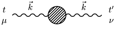
Figure 3: The in-medium contribution $\delta{\cal G}_{\mu\nu}(t,t^{\prime};{\vec{k}})$ to the non-equilibrium photon propagator at lowest order in the electromagnetic coupling constant $e$. Wavy lines represent the free vacuum photon propagator and the dashed blob represents the unequal-time current-current correlator which, at this order, corresponds to the non-equilibrium in-medium photon polarization tensor $\Pi_{\mu\nu}$.

The lowest order in-medium contribution to the photon propagator (40) represented on Fig. 3 reads:

$$\delta{\cal G}_{\mu\nu}(t,t^{\prime};{\vec{k}})=-\int_{\cal C}dudv\,G_{\mu\rho}(t,u;{\vec{k}})\,\Pi^{\rho\sigma}(u,v;{\vec{k}})\,G_{\sigma\nu}(v,t^{\prime};{\vec{k}})\,,$$ (40)

with time integrals along the contour of Fig. 2. The free vacuum photon propagator reads, in Feynman gauge:

$$G_{\mu\nu}(t,t^{\prime};{\vec{q}})=-g_{\mu\nu}\,G(t,t^{\prime};{\vec{k}})\,,$$ (41)

with (see Eqs. (21) and (22))

$$G^{>}(t,t^{\prime};{\vec{k}}) = \frac{1}{2k}\,{\rm e}^{-ik(t-t^{\prime})}$$ (42)

$$G^{<}(t,t^{\prime};{\vec{k}}) = \frac{1}{2k}\,{\rm e}^{ik(t-t^{\prime})}\,.$$ (43)

Writing explicitly the time integrals along the contour, we obtain:

$$\delta{\cal G}_{\mu\nu}^{<}(t,t^{\prime};{\vec{k}})=-\int_{-\infty}^{t}[du]\int_{-\infty}^{t^{\prime}}[dv]\,G_{\rho}(t,u;{\vec{k}})\,\Pi^{<}_{\mu\nu}(u,v;{\vec{k}})\,G_{\rho}(v,t^{\prime};{\vec{k}})$$

$$+\int_{-\infty}^{t}[du]\int_{-\infty}^{u}[dv]\,G_{\rho}(t,u;{\vec{k}})\,\Pi^{\rho}_{\mu\nu}(u,v;{\vec{k}})\,G^{<}(v,t^{\prime};{\vec{k}})$$

$$+\int_{-\infty}^{t^{\prime}}[du]\int_{u}^{t^{\prime}}\,\,[dv]\,G^{<}(t,u;{\vec{k}})\,\Pi^{\rho}_{\mu\nu}(u,v;{\vec{k}})\,G_{\rho}(v,t^{\prime};{\vec{k}}) \!\!\!\!\!\!,$$ (44)

where we used the notation (18) and where we introduced the so-called spectral component of the various two-point functions:

$$\Pi_{\mu\nu}^{\rho}(t,t^{\prime};{\vec{k}})=i\,\Big{(}\Pi_{\mu\nu}^{>}(t,t^{\prime};{\vec{k}})-\Pi_{\mu\nu}^{<}(t,t^{\prime};{\vec{k}})\Big{)}$$ (45)

and similarly for the free propagator:

$$G_{\rho}(t,t^{\prime};{\vec{k}})=i\,\Big{(}G^{>}(t,t^{\prime};{\vec{k}})-G^{<}(t,t^{\prime};{\vec{k}})\Big{)}=\frac{\sin k(t-t^{\prime})}{k}\,.$$ (46)

Working out the time derivatives in Eq. (31), we obtain the following expression for the single-photon inclusive spectrum at time $t$:

$$2k\,\frac{dn_{\gamma}(t,{\vec{k}})}{d^{3}x\,d^{3}k}=\frac{1}{(2\pi)^{3}}\,\int_{-\infty}^{t}[du][dv]\,{\rm e}^{-ik(u-v)}\,\gamma^{\mu\nu}({\vec{k}})\,\Pi^{<}_{\nu\mu}(v,u;{\vec{k}})\,.$$ (47)

We end this subsection by mentioning that the above expression (3.1) for the in-medium contribution to the photon propagator can be rewritten in a more compact form, which will prove useful for later use:

$$\delta{\cal G}_{\mu\nu}^{<}(t,t^{\prime};{\vec{k}})=\int_{-\infty}^{+\infty}[du][dv]\,\Big{\{}\,\,G_{R}(t,u;{\vec{k}})\,\Pi^{<}_{\mu\nu}(u,v;{\vec{k}})\,G_{A}(v,t^{\prime};{\vec{k}})$$

$$+G_{R}(t,u;{\vec{k}})\,\Pi^{R}_{\mu\nu}(u,v;{\vec{k}})\,G^{<}(v,t^{\prime};{\vec{k}})$$

$$+G^{<}(t,u;{\vec{k}})\,\Pi^{A}_{\mu\nu}(u,v;{\vec{k}})\,G_{A}(v,t^{\prime};{\vec{k}}) \!\Big{\}}\,,$$ (48)

where we introduced the retarded and advanced components:

$$\Pi^{R}_{\mu\nu}(t,t^{\prime};{\vec{k}}) = \Theta(t-t^{\prime})\,\Pi^{\rho}_{\mu\nu}(t,t^{\prime};{\vec{k}})$$ (49)

$$\Pi^{A}_{\mu\nu}(t,t^{\prime};{\vec{k}}) = -\Theta(t^{\prime}-t)\,\Pi^{\rho}_{\mu\nu}(t,t^{\prime};{\vec{k}})\,,$$ (50)

and similarly for the free propagator $G$.

3.2 Alternative derivation and physical interpretation

Here, we present an alternative derivation of the formula (47) for the inclusive photon spectrum, not using the virtual negative time evolution formalism introduced in the previous section. For this purpose, we work in the basis where the density matrix $\rho_{\rm s}$ of the system is diagonal (we use Greek letters to label the corresponding states throughout this subsection):

$$\rho_{\rm s}=\sum_{\alpha}P^{\rm s}_{\alpha}|\alpha,{\rm s}\rangle\langle\alpha,{\rm s}|\,,$$ (51)

where $\langle\alpha,{\rm s}|\,\rho_{\rm s}\,|\beta,{\rm s}\rangle=\delta_{\alpha\beta}\,P^{\rm s}_{\alpha}$.

Let us first focus on a particular state $|\alpha,{\rm s}\rangle$ of this statistical ensemble and construct the corresponding dressed initial state $|\alpha\rangle$ at time $t=0$. At ${\cal O}(e)$, the latter consists of a superposition of the bare zero-photon state and of all one-photon states allowed by the dynamics (the photon cloud). Making use of the adiabatic representation (5), it can be expressed as:

$$|\alpha\rangle = \Big{\{}1-i\int_{-\infty}^{0}du\,{\rm e}^{\epsilon u}\,H_{\rm I}(u)\Big{\}}|\alpha,{\rm s}\rangle\otimes|0,{\rm em}\rangle$$ (52)

$$= |\alpha,{\rm s}\rangle\otimes|0,{\rm em}\rangle+V\!\int\frac{d^{3}k}{(2\pi)^{3}}\sum_{\lambda=0}^{3}\sum_{\beta}\,\Phi^{(\lambda)}_{\beta\alpha}({\vec{k}})\,|\beta,{\rm s}\rangle\otimes|(\lambda,{\vec{k}}),{\rm em}\rangle$$

where

$$|(\lambda,{\vec{k}}),{\rm em}\rangle\equiv a_{\lambda}^{\dagger}({\vec{k}})|0,{\rm em}\rangle$$ (53)

is the one-photon state with polarization $\lambda$ and momentum ${\vec{k}}$. The wave-function $\Phi^{(\lambda)}_{\alpha\beta}({\vec{k}})$ is given by the appropriate matrix element of the interaction Hamiltonian (24), which reads explicitly:

$$i\Phi^{(\lambda)}_{\beta\alpha}({\vec{k}})=\int_{-\infty}^{0}du\,{\rm e}^{\epsilon u}\,{\rm e}^{iku}\frac{\epsilon^{(\lambda)}_{\mu}({\vec{k}})}{\sqrt{2k}}\,\langle\beta,{\rm s}|J_{\rm s}^{\mu}(u,{\vec{k}})|\alpha,{\rm s}\rangle\,.$$ (54)

The probability amplitude of having at least one photon with (transverse) polarization $\lambda$ and momentum ${\vec{k}}$ at time $t$ is obtained by evolving the state (52) up to time $t$ with the full Hamiltonian $H$ and by projecting over all possible final states containing at least the desired photon. At leading order in $e$, only one-photon final states contribute and the associated probability amplitude consists of two distinct pieces corresponding to the cases where: (1) the measured photon is actually produced during the time evolution from $t=0$ to $t$ ; (2) the measured photon was already present in the initial virtual cloud. Below, we construct the two corresponding amplitudes at lowest order in $e$:

(1) the measured photon is produced between times $t=0$ and $t$. This corresponds to the case where one starts in the zero-photon part $|\alpha,{\rm s}\rangle\otimes|0,{\rm em}\rangle$ of the initial state (52). The corresponding amplitude can be obtained by the following sequence: First, the unperturbed time evolution from the initial state $|\alpha,{\rm s}\rangle\otimes|0,{\rm em}\rangle$ at $t=0$ to an intermediate state $|i,{\rm s}\rangle\otimes|0,{\rm em}\rangle$ at the intermediate time $0\leq u\leq t$. The associated amplitude is given by the corresponding matrix element of the unperturbed evolution operator $\exp(-i[H_{\rm s}+H_{\rm em}]t)$, which reduces to:

$$\langle i,{\rm s}|{\rm e}^{-iH_{\rm s}\,u}|\alpha,{\rm s}\rangle\,.$$ (55)

Second, the transition from the state $|i,{\rm s}\rangle\otimes|0,{\rm em}\rangle$ to one of the possible one-photon states $|j,{\rm s}\rangle\otimes|(\lambda,{\vec{k}}),{\rm em}\rangle$ allowed by the dynamics. The corresponding transition amplitude is given by the matrix element of the interaction Hamiltonian (24) between these states:

$$\frac{\epsilon^{(\lambda)}_{\mu}({\vec{k}})}{\sqrt{2k}}\,\langle j,{\rm s}|J^{\mu}({\vec{k}})|i,{\rm s}\rangle\,.$$ (56)

Finally, the time-evolution from state $|j,{\rm s}\rangle\otimes|(\lambda,{\vec{k}}),{\rm em}\rangle$ at time $u$ to the final state $|\beta,{\rm s}\rangle\otimes|(\lambda,{\vec{k}}),{\rm em}\rangle$, at time $t$, with the amplitude

$${\rm e}^{-ik(t-u)}\,\langle\beta,{\rm s}|{\rm e}^{-iH_{\rm s}(t-u)}|j,{\rm s}\rangle\,.$$ (57)

where the phase factor corresponds to the free propagation of the one-photon state.

Integrating over all possible times of emission and summing over all possible intermediate states, one obtains the amplitude:

$${\cal A}^{(\lambda)}_{1,\alpha\rightarrow\beta}(t,{\vec{k}})=\frac{1}{\sqrt{2k}}\,\int_{0}^{t}du\,{\rm e}^{-ik(t-u)}\,\langle\beta,{\rm s}|{\rm e}^{-iH_{\rm s}t}\,\epsilon^{(\lambda)}({\vec{k}})\cdot J_{\rm s}(u,{\vec{k}})|\alpha,{\rm s}\rangle\,.$$ (58)

where we used the definition (39).

(2) the measured photon is part of the initial virtual cloud. In that case, it freely propagates from time $t=0$ to time $t$. The amplitude corresponding to the transition from a given one-photon states $|\delta,{\rm s}\rangle\otimes|(\lambda,{\vec{k}}),{\rm em}\rangle$ of the virtual cloud in (52) at time $t=0$ to the final state $|\beta,{\rm s}\rangle\otimes|(\lambda,{\vec{k}}),{\rm em}\rangle$ at time $t$ reads:

$${\rm e}^{-ikt}\,\langle\beta,{\rm s}|{\rm e}^{-iH_{\rm s}t}|\delta,{\rm s}\rangle\,.$$ (59)

Summing over the possible states of the virtual cloud weighted with the associated wave-function (54), one obtains the final amplitude:

$${\cal A}^{(\lambda)}_{2,\alpha\rightarrow\beta}(t,{\vec{k}}) = \sum_{\delta}\,{\rm e}^{-ikt}\,\langle\beta,{\rm s}|{\rm e}^{-iH_{\rm s}t}|\delta,{\rm s}\rangle\times\Phi^{(\lambda)}_{\delta\alpha}({\vec{k}})$$ (60)

$$= \frac{1}{\sqrt{2k}}\,\int_{-\infty}^{0}du\,{\rm e}^{\epsilon u}\,{\rm e}^{-ik(t-u)}\,\langle\beta,{\rm s}|{\rm e}^{-iH_{\rm s}t}\,\epsilon^{(\lambda)}({\vec{k}})\cdot J_{\rm s}(u,{\vec{k}})|\alpha,{\rm s}\rangle\,.$$

Putting everything together we get, for the total amplitude:

$${\cal A}^{(\lambda)}_{\alpha\rightarrow\beta}(t,{\vec{k}}) = {\cal A}^{(\lambda)}_{1,\alpha\rightarrow\beta}(t,{\vec{k}})+{\cal A}^{(\lambda)}_{2,\alpha\rightarrow\beta}(t,{\vec{k}})$$ (61)

$$= \frac{1}{\sqrt{2k}}\,\int_{-\infty}^{t}[du]\,{\rm e}^{-ik(t-u)}\,\langle\beta,{\rm s}|{\rm e}^{-iH_{\rm s}t}\,\epsilon^{(\lambda)}({\vec{k}})\cdot J_{\rm s}(u,{\vec{k}})|\alpha,{\rm s}\rangle\,.$$

Squaring this amplitude to get the associated probability and summing over all possible final states $|\beta,{\rm s}\rangle$ as well as over transverse polarizations, one obtains the desired inclusive spectrum corresponding to the initial state (52). Finally, averaging over all possible initial states $|\alpha,{\rm s}\rangle$ with the appropriate weight $P^{\rm s}_{\alpha}$, we recover our previous result, Eq. (47), for the inclusive spectrum:

$$(2\pi)^{3}\,\frac{dn_{\gamma}(t,{\vec{k}})}{d^{3}x\,d^{3}k}=\sum_{\alpha}P^{\rm s}_{\alpha}\,\left(\sum_{\lambda=\perp}\sum_{\beta}\Big{|}{\cal A}^{(\lambda)}_{\alpha\rightarrow\beta}(t,{\vec{k}})\Big{|}^{2}\right)$$ (62)

Therefore, we see that the various contributions to Eq. (47) corresponding to the various parts of the time integrations can be given very simple interpretations. Writing schematically (we omit the $\epsilon$–terms):

$$\int_{-\infty}^{t}[du]\,[dv]\equiv\int_{-\infty}^{0}du\,\int_{-\infty}^{0}dv\,+\int_{-\infty}^{0}du\,\int_{0}^{t}dv+\int_{0}^{t}du\int_{-\infty}^{0}dv\,+\int_{0}^{t}du\int_{0}^{t}dv\,,$$ (63)

we see, in the light of the previous discussion, that the contribution from negative times ($u,v\leq 0$) corresponds to the probability that the photon in the final state was already present in the initial virtual cloud. Similarly, the contribution from purely positive times ($u,v\geq 0$) corresponds to the probability that the measured photon has actually been produced between times $t=0$ and $t$. Finally, the cross-terms, which involve integrations over both negative and positive times, describe the interference between these two possibilities. Notice that the latter depends explicitly on time and, as a consequence, contributes to the actual production rate (see below).

3.3 Photon production rate and spectrum of produced photons

One obtains the out-of-equilibrium photon production rate at a given time $t$, by taking the time-derivative of Eq. (47). The complete expression at lowest order in $e$ is, therefore:

$$2k\,\frac{dn_{\gamma}(t,{\vec{k}})}{d^{4}x\,d^{3}k}=\frac{1}{(2\pi)^{3}}\,\int_{-\infty}^{t}[du]\,2{\rm Re}\Big{\{}{\rm e}^{ik(t-u)}\,\gamma^{\mu\nu}({\vec{k}})\,\Pi^{<}_{\mu\nu}(t,u;{\vec{k}})\Big{\}}\,,$$ (64)

where we used the fact that: $\Pi^{<}_{\mu\nu}(t,t^{\prime};{\vec{k}})=\Pi^{<\,*}_{\nu\mu}(t^{\prime},t;{\vec{k}})$. Equation (64) relates the photon production rate to the intrinsic dynamical properties of the out-of-equilibrium emitting system, which are characterized at this order by the unequal-time photon polarization tensor $\Pi^{<}_{\mu\nu}(t,u;{\vec{k}})$. This generalizes the corresponding equilibrium formula [1, 45, 46] (see Eq. (97) below).

The inclusive spectrum of actually produced photons can be obtained from Eq. (47) by subtracting the contribution from the initial virtual cloud, which is simply given by Eq. (47) itself, written at $t=0$:

$$\frac{dn_{\gamma}(t,{\vec{k}})}{d^{3}x\,d^{3}k}\Big{|}_{\rm prod}\equiv\frac{dn_{\gamma}(t,{\vec{k}})}{d^{3}x\,d^{3}k}-\frac{dn_{\gamma}(0,{\vec{k}})}{d^{3}x\,d^{3}k}$$ (65)

This is, of course, equivalent to a direct integration of the production rate (64) from $t=0$ to $t$, namely:

$$\frac{dn_{\gamma}(t,{\vec{k}})}{d^{3}x\,d^{3}k}\Big{|}_{\rm prod}=\int_{0}^{t}dt^{\prime}\,\frac{dn_{\gamma}(t^{\prime},{\vec{k}})}{d^{4}x\,d^{3}k}\,.$$ (66)

Notice that, although the contribution from the virtual cloud has been subtracted, there still remains a time integral over infinite negative times in Eq. (64). As we have seen previously, this corresponds to interference effects with the virtual cloud.

3.4 Inclusive spectrum of correlated lepton pairs at time $t$

We now come to the case of dilepton production. The density of correlated lepton pairs with momenta ${\vec{k}}$ (lepton) and ${\vec{p}}$ (anti-lepton) at time $t$ is given by

$$\frac{dn_{\ell^{+}\ell^{-}}(t,{\vec{k}},{\vec{p}})}{d^{3}x\,d^{3}k\,d^{3}p}=\frac{V}{(2\pi)^{6}}\,\sum_{\sigma,\sigma^{\prime}}\Big{<}N^{\ell^{-}}_{\sigma}(t,{\vec{k}})\,N^{\ell^{+}}_{\sigma^{\prime}}(t,{\vec{p}})\Big{>}\,,$$ (67)

where the RHS is to be understood as a connected correlator. Here $V\equiv(2\pi)^{3}\,\delta^{(3)}(\vec{0})$ is the quantization volume and

$$N^{\ell^{-}}_{\sigma}(t,{\vec{p}}) = b_{\sigma}^{\dagger}(t,{\vec{p}})\,b_{\sigma}(t,{\vec{p}})$$ (68)

$$N^{\ell^{+}}_{\sigma}(t,{\vec{p}}) = d_{\sigma}^{\dagger}(t,{\vec{p}})\,d_{\sigma}(t,{\vec{p}})$$ (69)

denote the Heisenberg picture number operators for leptons and anti-leptons with momentum ${\vec{p}}$ and spin projection $\sigma=\pm$. In terms of the Fourier modes of the lepton field operators

$$\psi(t,{\vec{k}}) = \frac{1}{\sqrt{V}}\,\int d^{3}x\,{\rm e}^{-i{\vec{k}}\cdot{\vec{x}}}\,\psi(t,{\vec{x}})$$ (70)

$$\bar{\psi}(t,{\vec{k}}) = \frac{1}{\sqrt{V}}\,\int d^{3}x\,{\rm e}^{i{\vec{k}}\cdot{\vec{x}}}\,\bar{\psi}(t,{\vec{x}})\,,$$ (71)

the relevant correlator is given by the following connected four-point function:

$$\sum_{\sigma,\sigma^{\prime}}\Big{<}N^{\ell^{-}}_{\sigma}(t,{\vec{k}})\,N^{\ell^{+}}_{\sigma^{\prime}}(t,{\vec{p}})\Big{>} = \Big{<}{\rm tr}\Big{\{}\bar{\psi}(t,{\vec{k}})\,\gamma_{0}\,\frac{K\!\!\!\!/\,+m}{2E_{k}}\,\gamma_{0}\,\psi(t,{\vec{k}})\Big{\}}$$ (72)

$$\times{\rm tr}\Big{\{}\gamma_{0}\,\frac{P\!\!\!\!/\,-m}{2E_{p}}\,\gamma_{0}\,\psi(t,-{\vec{p}})\,\bar{\psi}(t,-{\vec{p}})\Big{\}}\Big{>}\,,$$

where $m$ is the lepton mass, $E_{k}=\sqrt{k^{2}+m^{2}}$, $E_{p}=\sqrt{p^{2}+m^{2}}$, $K^{\mu}\equiv(E_{k},{\vec{k}})$, $P^{\mu}\equiv(E_{p},{\vec{p}})$, $K\!\!\!\!/\,=\gamma^{\mu}K_{\mu}$ and $P\!\!\!\!/\,=\gamma^{\mu}P_{\mu}$. This correlator can be computed using the method described in section 2. As in the case of photons the purely leptonic contributions, involving the lepton current $j^{\mu}$ only, vanish identically. Here, we focus on medium contributions, which involve $J^{\mu}$ at least once. The first non-vanishing medium contributions occur at ${\cal O}(e^{4})$ and involve the unequal-time current-current correlator (38). There are two possible topologies at this order, one of which is represented on Fig. 4, where the lines represent the free lepton propagator on the contour ${\cal C}$:

$$D(t,t^{\prime};{\vec{k}})=\Big{<}T_{\cal C}\Big{\{}\psi_{\rm em}(t,{\vec{k}})\,\bar{\psi}_{\rm em}(t^{\prime},{\vec{k}})\Big{\}}\Big{>}_{\rm em}\,.$$ (73)

As we did previously for the photon field, we have renamed the interaction picture of lepton field operators as follows:

$$\psi_{\rm em}(t,{\vec{k}})\equiv\psi_{\,{\rm I}}(t,{\vec{k}})={\rm e}^{iH_{\rm em}t}\,\psi({\vec{k}})\,{\rm e}^{-iH_{\rm em}t}\,,$$ (74)

and likewise for $\bar{\psi}_{\rm em}(t,{\vec{k}})$. With initial conditions corresponding to Eq. (23), the components of the lepton propagator are given by:

$$D^{>}(t,t^{\prime};{\vec{k}}) = \frac{K\!\!\!\!/\,+m}{2E_{k}}\,{\rm e}^{-iE_{k}(t-t^{\prime})}$$ (75)

$$D^{<}(t,t^{\prime};-{\vec{k}}) = \frac{K\!\!\!\!/\,-m}{2E_{k}}\,{\rm e}^{iE_{k}(t-t^{\prime})}\,.$$ (76)

Figure 4: The lowest order medium contribution to dilepton production. The dashed blob represents the ${\cal O}(e^{2})$ in-medium photon polarization tensor. Lepton momenta follow the fermionic flow.

The contribution depicted in Fig. 4 can be expressed in terms of the lowest order in-medium contribution to the photon propagator $\delta{\cal G}_{\mu\nu}$, represented on Fig. 3 (see Eq. (40)):

$$V\cdot\sum_{\sigma,\sigma^{\prime}}\Big{<}N^{\ell^{-}}_{\sigma}(t,{\vec{k}})\,N^{\ell^{+}}_{\sigma^{\prime}}(t,{\vec{p}})\Big{>}=-e^{2}\,\int_{\cal C}dudv\,l^{\mu\nu}(t,u,v;{\vec{k}},{\vec{p}})\,\delta{\cal G}_{\nu\mu}(v,u;{\vec{q}})\,,$$ (77)

where ${\vec{q}}={\vec{k}}+{\vec{p}}$ is the total momentum of the lepton pair and where

$$l^{\mu\nu}(t,u,v;{\vec{k}},{\vec{p}}) = {\rm tr}\Big{\{}D(t,u;-{\vec{p}})\gamma^{\mu}\,D(u,t;{\vec{k}})\,\gamma_{0}\,\frac{K\!\!\!\!/\,+m}{2E_{k}}\,\gamma_{0}$$ (78)

$$\quad\times D(t,v;{\vec{k}})\,\gamma^{\nu}\,D(v,t;-{\vec{p}})\,\gamma_{0}\,\frac{P\!\!\!\!/\,-m}{2E_{p}}\,\gamma_{0}\,\Big{\}}\,.$$

Writing explicitly the time integrations along the contour and making use of Eqs. (75)-(76), one can perform the trace over Dirac indices. A lengthy but straightforward calculation shows that all but one of the contributions on the contour vanish. A similar calculation shows that the other possible contribution to the fermion four-point function gives a vanishing contribution to dilepton production after performing the relevant projections on positive and negative energy final states. Putting everything together, we finally obtain the following expression for the inclusive spectrum of correlated lepton pairs at time $t$, at leading order in the electromagnetic coupling constant:

$$\frac{dn_{\ell^{+}\ell^{-}}(t,{\vec{k}},{\vec{p}})}{d^{3}x\,d^{3}k\,d^{3}p}=\frac{e^{2}}{(2\pi)^{6}}\,\int_{-\infty}^{t}[du][dv]\,{\rm e}^{-i(E_{k}+E_{p})(u-v)}\,\ell^{\mu\nu}({\vec{k}},{\vec{p}})\,\delta{\cal G}^{<}_{\nu\mu}(v,u;{\vec{q}})\,,$$ (79)

where

$$\ell_{\mu\nu}({\vec{k}},{\vec{p}})=\frac{K_{\mu}P_{\nu}+P_{\mu}K_{\nu}-g_{\mu\nu}(K\cdot P+m^{2})}{E_{k}\,E_{p}}\,.$$ (80)

is the usual vacuum lepton tensor [41]. One obtains the number of correlated pairs with total four-momentum $Q^{\mu}=(q_{0},{\vec{q}})$ by integrating (79) over momenta with the constraints ${\vec{p}}+{\vec{k}}={\vec{q}}$ and $E_{p}+E_{k}=q_{0}$. Using

$$\int\frac{d^{3}k}{(2\pi)^{3}}\frac{d^{3}p}{(2\pi)^{3}}\,(2\pi)^{4}\,\delta^{(4)}(Q-P-K)\,\ell_{\mu\nu}({\vec{k}},{\vec{p}})\,{\rm e}^{i(E_{k}+E_{p})t}=L_{\mu\nu}(Q^{2})\,{\rm e}^{iq_{0}t}\,,$$ (81)

where ($Q^{2}\geq 4m^{2}$)

$$L_{\mu\nu}(Q^{2})=\frac{1}{6\pi}\,\Big{(}1+\frac{2m^{2}}{Q^{2}}\Big{)}\,\Big{(}1-\frac{4m^{2}}{Q^{2}}\Big{)}^{\!\frac{1}{2}}\,[Q_{\mu}Q_{\nu}-g_{\mu\nu}Q^{2}]\,,$$ (82)

we obtain:

$$\frac{dn_{\ell^{+}\ell^{-}}(t,q_{0},{\vec{q}})}{d^{3}x\,d^{4}Q}=\frac{e^{2}}{(2\pi)^{4}}\,\int_{-\infty}^{t}[du][dv]\,{\rm e}^{-iq_{0}(u-v)}\,L^{\mu\nu}(Q^{2})\,\delta{\cal G}^{<}_{\nu\mu}(v,u;{\vec{q}})\,.$$ (83)

Note that the general structure of the expressions (79) and (83) is very similar to that obtained in the case of photon production, Eq. (47). In particular, the integrand does not explicitly depend on $t$ and the time-dependence only appears through the upper bound of the time integrations. Following the line of reasoning of section 3.2, the various integrations over negative and positive times involved in Eqs. (79), (83) and (3.1) can be given simple physical interpretations. At lowest order in $e$, the basic process is the emission of an off-shell photon which decays into a lepton pair and the probability amplitude for having (at least) a lepton pair in the final state can be decomposed in various pieces corresponding to the various possible times of emission and decay of the off-shell photon. For instance, the pair may already be present in the virtual cloud, which correspond to both times being negative, or an off-shell photon from the virtual cloud may decay between $t=0$ and $t$, etc. The various pieces of the time integrations in Eqs. (79), (83) and (3.1) correspond either to the probabilities associated with each possibility or to the interferences between different possibilities.

3.5 Dilepton production rate and spectrum of produced pairs

As in the case of photon production, one obtains the rate of lepton pair production as a function of time by taking the time derivative of expressions (79) and (83) above. We get, for pairs of lepton and anti-lepton with momenta ${\vec{k}}$ and ${\vec{p}}$ respectively:

$$\frac{dn_{\ell^{+}\ell^{-}}(t,{\vec{k}},{\vec{p}})}{d^{4}x\,d^{3}k\,d^{3}p}=\frac{e^{2}}{(2\pi)^{6}}\,\int_{-\infty}^{t}[du]\,2{\rm Re}\Big{\{}{\rm e}^{i(E_{p}+E_{k})(t-u)}\,\ell^{\mu\nu}({\vec{k}},{\vec{p}})\,\delta{\cal G}^{<}_{\mu\nu}(t,u;{\vec{q}})\Big{\}}\,,$$ (84)

and, for a pair with total four momentum $Q$:

$$\frac{dn_{\ell^{+}\ell^{-}}(t,q_{0},{\vec{q}})}{d^{4}x\,d^{4}Q}=\frac{e^{2}}{(2\pi)^{4}}\,\int_{-\infty}^{t}[du]\,2{\rm Re}\Big{\{}{\rm e}^{iq_{0}(t-u)}\,L^{\mu\nu}(Q^{2})\,\delta{\cal G}^{<}_{\mu\nu}(t,u;{\vec{q}})\Big{\}}\,.$$ (85)

The number of produced pairs at time $t$ is obtained either by subtracting the virtual contribution ($t=0$) from expressions (79) and (83) or by integrating the above rates from $t=0$ to $t$. For instance:

$$\frac{dn_{\ell^{+}\ell^{-}}(t,q_{0},{\vec{q}})}{d^{3}x\,d^{4}Q}\Big{|}_{\rm prod}=\int_{0}^{t}dt^{\prime}\,\frac{dn_{\ell^{+}\ell^{-}}(t^{\prime},q_{0},{\vec{q}})}{d^{4}x\,d^{4}Q}\,.$$ (86)

3.6 Charged scalar fields

We end this section by considering how the above formulas for the photon and dilepton production rates are modified in the case where the emitting system contains charged scalar fields such as e.g. charged pions. This is of interest e.g. in the hadronic phase in heavy ion collisions, or during the out-of-equilibrium chiral phase transition, where so-called disoriented chiral condensates might occasionally form, leading to coherent pion emission [22]. The accompanied electromagnetic radiation might provide an interesting signature of this phenomenon [23, 24].

Apart from the contribution of charged scalar field to the current (26), the electromagnetic interaction Hamiltonian (24) now contains an additional contribution of the type:

$$H_{\rm int}^{\rm scal}=e^{2}\,\int d^{3}x\,A^{\mu}({\vec{x}})A_{\mu}({\vec{x}})\,\phi^{\dagger}({\vec{x}})\phi({\vec{x}})\,,$$ (87)

where $\phi({\vec{x}})$ denotes the charged scalar field operator. Repeating the above analysis for photon and dilepton production, it is easy to see that, at lowest order in $e$, the presence of this “two-photon” vertex simply amounts to an additional tadpole-like contribution to the expression (40) of the in-medium photon polarization tensor. It can be formally obtained from Eq. (40) by replacing $\Pi_{\mu\nu}(u,v;{\vec{q}})$ by $-i\,{\rm K}(u)\,g_{\mu\nu}\,\delta_{\cal C}(u-v)$, where

$${\rm K}(t)=e^{2}\,\int\frac{d^{3}k}{(2\pi)^{3}}\,\langle\varphi_{\rm s}^{\dagger}(t,{\vec{k}})\,\varphi_{\rm s}(t,{\vec{k}})\rangle_{\rm s}\,,$$ (88)

with $\varphi_{\rm s}(t,{\vec{k}})$ the interaction picture of the Fourier modes of the field operator (see Eq. (12)):

$$\varphi_{\rm s}(t,{\vec{k}})\equiv\varphi_{\rm I}(t,{\vec{k}})={\rm e}^{iH_{\rm s}t}\,\varphi({\vec{k}})\,{\rm e}^{-iH_{\rm s}t}\,,$$ (89)

where ($V$ is the normalization volume)

$$\varphi({\vec{k}})=\frac{1}{\sqrt{V}}\,\int d^{3}x\,{\rm e}^{-i{\vec{k}}\cdot{\vec{x}}}\,\phi({\vec{x}})\,.$$ (90)

Writing explicitly the time integrals along the contour, one obtains that, in presence of scalar fields, the tadpole contribution to Eq. (3.1) reads:

$$\delta{\cal G}_{\mu\nu}^{<}(t,t^{\prime};{\vec{q}})\Big{|}_{\rm tadpole} = g_{\mu\nu}\,\int_{-\infty}^{t}[du]\,G_{\rho}(t,u;{\vec{q}})\,{\rm K}(u)\,G^{<}(u,t^{\prime};{\vec{q}})$$ (91)

$$- g_{\mu\nu}\,\int_{-\infty}^{t^{\prime}}[du]\,G^{<}(t,u;{\vec{q}})\,{\rm K}(u)\,G_{\rho}(u,t^{\prime};{\vec{q}})\,.$$

Using the expressions (42), (43) and (46) of free propagators, it is straightforward to show that the tadpole term does not contribute to photon production:

$$\lim_{t^{\prime}\rightarrow t}\,\,\Big{(}\partial_{t}\partial_{t^{\prime}}+ik(\partial_{t}-\partial_{t^{\prime}})+k^{2}\Big{)}\,\delta{\cal G}_{\mu\nu}^{<}(t,t^{\prime};{\vec{k}})\Big{|}_{\rm tadpole}=0\,.$$ (92)

However, in general it gives a non-vanishing contribution to the out-of-equilibrium dilepton production. We stress that this contribution results from the non-trivial time-evolution of the emitting system. In particular, it vanishes identically in equilibrium and, more generally, for any stationary state, as we will show below. It is, therefore, a genuine non-equilibrium effect.

4 Applications

In this section, we apply the general formulas derived above to the case of time-translation invariant (stationary) systems. In particular, we recover known expressions for the production rates in thermodynamic equilibrium. We also show that a consistent description of the initial virtual cloud guarantees that only on-shell processes contribute to production rates in the case of stationary systems and that the vacuum is stable against spontaneous emission. These provide important checks of the physical consistency of the present description. Finally, we consider the case of quasi-stationary systems and work out, in particular, the first non-trivial corrections to the local expression of the photon production rate – used e.g. in hydrodynamic calculations – in a standard gradient expansion.

4.1 Recovering known formulas for stationary systems

It is instructive to reproduce the usual equilibrium expressions for the photon and dilepton production rates from the general out-of-equilibrium expressions derived above. For this purpose, we consider the case where the emitting system undergoes a stationary evolution. This is the case whenever the initial condition does not break time-translation invariance, that is when the density matrix $\rho_{\rm s}$ commutes with the Hamiltonian $H_{\rm s}$ (it can, therefore, be diagonalized in the basis of eigenstates $|n,{\rm s}\rangle$, cf. Eq. (1)):

$$[\rho_{\rm s};H_{\rm s}]=0\,\Leftrightarrow\,P^{\rm s}_{nm}=P^{\rm s}_{n}\,\delta_{m,n}\,.$$ (93)

In that case, all correlation functions only depend on time differences and it is useful to work in frequency space. In particular, one has:

$$\Pi^{<}_{\mu\nu}(t,t^{\prime};{\vec{k}})\equiv\Pi^{<}_{\mu\nu}(t-t^{\prime};{\vec{k}})=\int_{-\infty}^{+\infty}\frac{d\omega}{2\pi}\,{\rm e}^{-i\omega(t-t^{\prime})}\,\bar{\Pi}^{<}_{\mu\nu}(\omega,{\vec{k}})\,,$$ (94)

and similarly for other two-point functions. Note the relation

$$\bar{\Pi}^{<\,*}_{\mu\nu}(\omega,{\vec{k}})=\bar{\Pi}^{<}_{\nu\mu}(\omega,{\vec{k}})\,.$$ (95)

Plugging the definition (94) in Eq. (64) and using the identity:

$$\int_{-\infty}^{t}[du]\,{\rm e}^{i\alpha(t-u)}=\pi\,\delta(\alpha)+i\,{\cal P}\Big{(}\frac{1}{\alpha}\Big{)}\,,$$ (96)

where $\cal P$ denotes the principal part, one obtains the following expression for the (time independent) photon production rate:

$$2k\,\frac{dn_{\gamma}({\vec{k}})}{d^{4}x\,d^{3}k}=\frac{1}{(2\pi)^{3}}\,\gamma^{\mu\nu}({\vec{k}})\,\bar{\Pi}^{<}_{\mu\nu}(k,{\vec{k}})=-\frac{1}{(2\pi)^{3}}\,{\mbox{$\bar{\Pi}$}^{<\,\mu}}_{\mu}(k,{\vec{k}})\,.$$ (97)

In writing the second equality, we used the fact that $\bar{\Pi}_{\mu\nu}$ is transverse ($K^{\mu}=(k^{0},{\vec{k}})$):

$$K^{\mu}\,\bar{\Pi}_{\mu\nu}(k_{0},{\vec{k}})=0\,,$$ (98)

as a consequence of gauge invariance.

Similar considerations directly lead to the following formula for the production rate of dileptons with invariant mass $Q$ (see Eq. (85)):

$$\frac{dn_{\ell^{+}\ell^{-}}(q_{0},{\vec{q}})}{d^{4}x\,d^{4}Q}=\frac{e^{2}}{(2\pi)^{4}}\,L^{\mu\nu}(Q^{2})\,\bar{\delta\cal G}^{<}_{\mu\nu}(q_{0},{\vec{q}})\,,$$ (99)

where the function $\bar{\delta\cal G}^{<}$ is defined as in Eq. (94). It can be easily expressed in terms of the polarization tensor $\bar{\Pi}^{<}$ by using Eq. (3.1) which has the form of a convolution product in time and which, therefore, corresponds to an algebraic product in frequency space. This is, of course, nothing else but the fact that time-translation invariance is equivalent to energy (frequency) conservation. The various components of the free photon propagator (41) have the following expressions in frequency space:

$$\bar{G}^{<}(\omega,{\vec{q}}) = \frac{\pi}{q}\,\delta(\omega+q)$$ (100)

$$\bar{G}^{R}(\omega,{\vec{q}}) = \frac{-1}{(\omega+i\eta)^{2}-q^{2}}$$ (101)

$$\bar{G}^{A}(\omega,{\vec{q}}) = \frac{-1}{(\omega-i\eta)^{2}-q^{2}}$$ (102)

where $\eta\equiv 0^{+}$. The contributions corresponding to the last two terms of Eq. (3.1) contain $G^{<}_{\mu\nu}(q_{0},{\vec{q}})\propto\delta(q_{0}+q)$ and, therefore, give vanishing contributions for $q_{0}>0$. The additional tadpole contribution appearing in the case of scalar fields (see Eq. (91)) vanishes identically for the same reason. Using Eqs. (82) and (98), one finally obtains ($\alpha_{\rm em}=e^{2}/4\pi$):

$$\frac{dn_{\ell^{+}\ell^{-}}(Q)}{d^{4}x\,d^{4}Q}=-\frac{\alpha_{\rm em}}{24\pi^{4}\,Q^{2}}\,\Big{(}1+\frac{2m^{2}}{Q^{2}}\Big{)}\,\Big{(}1-\frac{4m^{2}}{Q^{2}}\Big{)}^{\!\frac{1}{2}}\,\,{\mbox{$\bar{\Pi}$}^{<\,\mu}}_{\mu}(q_{0},{\vec{q}})\,.$$ (103)

Equations. (97) and (103) are the usual expressions of the photon and dilepton production rates for general stationary situations. For the particular case of thermodynamic equilibrium at temperature $T=1/\beta$ these are usually expressed in terms of the spectral function $\bar{\Pi}^{\rho}_{\mu\nu}(q_{0},{\vec{q}})=2i\,{\rm Im}\bar{\Pi}^{R}_{\mu\nu}(q_{0},{\vec{q}})$ (see Eqs. (45), (49) and (50)) by making use of the detailed balance (or KMS) relation:

$$\bar{\Pi}^{>}_{\mu\nu}(q_{0},{\vec{q}})\Big{|}_{\rm eq}={\rm e}^{\beta q_{0}}\,\bar{\Pi}^{<}_{\mu\nu}(q_{0},{\vec{q}})\Big{|}_{\rm eq}\,,$$ (104)

from which it follows that

$$\bar{\Pi}^{<}_{\mu\nu}(q_{0},{\vec{q}})\Big{|}_{\rm eq}=\frac{2}{{\rm e}^{\beta q_{0}}-1}\,{\rm Im}\bar{\Pi}^{R}_{\mu\nu}(q_{0},{\vec{q}})\Big{|}_{\rm eq}\,.$$ (105)

Putting everything together, one recognizes the familiar expressions for the photon and dilepton production rates in equilibrium [1, 45, 46, 41].

As an important physical consequence, the above results guarantee that the vacuum is stable against spontaneous emission. Indeed, the fact that only on-shell (energy-conserving) processes contribute in stationary situations implies that:

$${\mbox{$\bar{\Pi}$}^{<\,\mu}}_{\mu}(q_{0},{\vec{q}})\Big{|}_{\rm vacuum}=0\,,$$ (106)

which can also be obtained as the zero temperature limit of Eq. (105). As a byproduct, this has the important implication that the purely leptonic contributions to the photon polarization tensor, which only involve the leptonic current $j^{\mu}$ and have, therefore, the structure of vacuum contributions, do not contribute to actual photon and dilepton production rates, as announced in section 3.

4.2 Slowly evolving systems: gradient expansion and off-shell effects

As mentioned in the introduction, a widely used ansatz for computing photon or dilepton production rates out of equilibrium is to use the above static formulas, Eqs (97) or (103), written at a given time $t$. One then supplement these local expressions for the production rates with a given modelization of the time-evolution of the system, like e.g. hydrodynamics, or an appropriate Boltzmann equation. This procedure might be justified if the typical time scale characterizing the process under study, say the formation time of the produced photon, is short compared to the time scale characterizing the time evolution of the system. In contrast, we clearly see from the expressions derived previously that in the general case the emission rates depend non-locally on the time history of the emitting system prior to the time of emission. It is therefore interesting to consider a somewhat intermediate situation where the system is slowly evolving (compared to the duration of the emission process) and to derive the first corrections to the static formulas, Eqs. (97) and (103). With the general expressions of the previous section in hand, we are in a position to work out these corrections by performing a standard gradient expansion. Here, we illustrate this point on the case of photon production.

Generalizing the notation introduced in Eq. (94), we introduce the Wigner transform in frequency space, that is a Fourier transform with respect to the time difference $t-t^{\prime}$ at fixed $T=\frac{1}{2}(t+t^{\prime})$:

$$\Pi^{<}_{\mu\nu}(t,t^{\prime};{\vec{k}})=\int\frac{d\omega}{2\pi}\,{\rm e}^{-i\omega(t-t^{\prime})}\,\bar{\Pi}^{<}_{\mu\nu}(T;\omega,{\vec{k}})\,,$$ (107)

and similarly for other two-point functions. Note that the relations (95) and (98) generalize:

$$\bar{\Pi}^{<\,*}_{\mu\nu}(T;\omega,{\vec{k}})=\bar{\Pi}^{<}_{\nu\mu}(T;\omega,{\vec{k}})\,,$$ (108)

and

$$K^{\mu}\,\bar{\Pi}_{\mu\nu}(T;k_{0},{\vec{k}})=0\,.$$ (109)

The photon production rate (64) can be rewritten as:

$$\frac{dn_{\gamma}(t,{\vec{k}})}{d^{4}x\,d^{3}k}=\int\frac{d\omega}{2\pi}\,\int_{-\infty}^{t}[du]\,\bar{\cal F}_{\gamma}(U;\omega,{\vec{k}})\,2{\rm Re}\Big{\{}{\rm e}^{i(k-\omega)(t-u)}\Big{\}},$$ (110)

where $U=\frac{1}{2}(t+u)$ and where we introduced the (real) function

$$\bar{\cal F}_{\gamma}(T;\omega,{\vec{k}})=\frac{\gamma^{\mu\nu}({\vec{k}})}{2k\,(2\pi)^{3}}\,\,\bar{\Pi}^{<}_{\mu\nu}(T;\omega,{\vec{k}})\,.$$ (111)

Writing $s=t-u$ and $U=t-\frac{1}{2}s$, and plugging the first order gradient expansion

$$\bar{\cal F}_{\gamma}(U;\omega,{\vec{k}})=\bar{\cal F}_{\gamma}(t;\omega,{\vec{k}})-\frac{1}{2}s\,\partial_{t}\bar{\cal F}_{\gamma}(t;\omega,{\vec{k}})+\ldots$$ (112)

in Eq. (110), one obtains, after simple manipulations and making use of Eq. (96):

$$\frac{dn_{\gamma}(t,{\vec{k}})}{d^{4}x\,d^{3}k}\simeq\bar{\cal F}_{\gamma}(t;k,{\vec{k}})+{\cal P}\int\frac{d\omega}{2\pi}\,\frac{\partial_{t}\bar{\cal F}_{\gamma}(t;\omega,{\vec{k}})}{(k-\omega)^{2}}\,.$$ (113)

Using Eqs. (35), (109) and (111), the first term of this expression reduces to the static expression (97) written at time $t$. This corresponds to the local ansatz described above. The second term represent the first non-trivial gradient correction arising from the finite duration of the emission process. As expected, it involves the off-shell part of the photon polarization tensor, which in turn involves energy non-conserving elementary processes.

5 The non-equilibrium photon polarization tensor

In the previous sections, we have related the time-dependent photon and dilepton production rates to the intrinsic dynamical properties of the out-of-equilibrium emitting medium which, at leading order in $e$, are characterized by the unequal-time current-current correlator (38). In the last part of this paper, we focus on the latter and discuss how it might be computed in general non-equilibrium situations. We first consider the issue of the negative time integration which involves the unequal-time correlation function of two current operators at positive and negative times. We propose a general method for the calculation of such unusual correlation functions, which is based on introducing a ${\cal S}$–shape path in real time. This might be combined with recently developed techniques in non-equilibrium quantum field theory in order to compute the explicit time dependence of the relevant correlation functions starting from a given initial condition. Finally, we briefly discuss how the photon polarization tensor can be obtained from the 2PI effective action.

5.1 General considerations: the ${\cal S}$-path

For the purpose of illustration, let us consider the case of photon production. Writing explicitly the various part of the time integration, the production rate (64) can be written as:

$$\frac{dn_{\gamma}(t,{\vec{k}})}{d^{4}x\,d^{3}k}=2{\rm Re}\left\{\,\int_{0}^{t}du\,{\rm e}^{ik(t-u)}\,{\cal F}_{\gamma}(t,u;{\vec{k}})+\int_{-\infty}^{0}du\,{\rm e}^{\epsilon u}\,{\rm e}^{ik(t-u)}\,{\cal F}_{\gamma}(t,u;{\vec{k}})\,\right\}\,,$$ (114)

where we denoted ${\cal F}_{\gamma}(t,u;{\vec{k}})=\frac{\gamma^{\mu\nu}({\vec{k}})}{2k(2\pi)^{3}}\,\Pi_{\mu\nu}(t,u;{\vec{k}})$. As discussed previously, the first term on the RHS of Eq. (114) describes the actual production of a photon between time $t=0$ and time $t$, while the second term corresponds to interferences with the initial virtual photon cloud. We see that the latter involves the correlation $\Pi_{\mu\nu}(t,u;{\vec{k}})$ (see Eq. (38)) between two current operators at positive time $t$ and negative time $u$ respectively. In practice, starting from a given initial condition, one therefore has to compute the time evolution of correlation functions of the emitting system in the positive as well as in the negative time direction (we recall that the latter is not a physical time evolution but merely a formal way of treating initial state correlations due to electromagnetic dressing). This can be done by introducing an appropriate contour in real time, such as, for instance, that of Fig. 2. The latter is, however, not well suited for practical calculation as it requires one to specify the initial state at $t=-\infty$. Here we shall introduce a different contour in real time which allows for a more useful formulation of the problem.

We consider a generic quantum field theory described by a set of fundamental (bosonic and/or fermionic) fields, which we collectively denote by $\varphi$. For the sake of the argument, we focus on the time-evolution of the system and omit all possible (Dirac, Lorentz, etc …) indices as well as spatial variables. Let us consider a general correlation function of two operators ${\cal O}$ at positive and negative times. We first notice that the operator with negative time argument can always be brought on the right of the one with positive time argument in the expressions of the production rates. The relevant correlation function can therefore be written ($t,t^{\prime}\geq 0$):

$$\langle{\cal O}_{\rm s}(t)\,{\cal O}_{\rm s}(-t^{\prime})\rangle_{\rm s}=\sum_{n,m}P^{\rm s}_{nm}\,\langle m,{\rm s}|\,{\cal U}(0,t)\,{\cal O}\,{\cal U}(t,0)\,{\cal U}(0,-t^{\prime})\,{\cal O}\,{\cal U}(-t^{\prime},0)|n,{\rm s}\rangle\,,$$ (115)

with the time-evolution operator

$${\cal U}(t,t^{\prime})={\rm e}^{-iH_{\rm s}(t-t^{\prime})}\,.$$ (116)

The above expression can be read as follows: Starting from a given state $|n,{\rm s}\rangle$ at time $t=0$, evolve the system backward in time up to time $-t^{\prime}$ and insert the operator ${\cal O}$; Then, evolve the system in the positive time direction from time $-t^{\prime}$ to time $t$ and insert ${\cal O}$ again; Finally, evolve the system back from time $t$ to time $t=0$ and compute the overlap with another state $|m,{\rm s}\rangle$. Repeat this for all possible states and average with the appropriate weight $P^{\rm s}_{nm}\equiv\langle n,{\rm s}|\,\rho_{\rm s}\,|m,{\rm s}\rangle$. It is easy to show that the calculation of such correlation function can be formulated by means of standard field theory methods by introducing a closed ${\cal S}$–shape contour along the real time axis, such as represented on Fig. 5. In particular, this can be given a path-integral formulation along the ${\cal S}$–path, allowing one to exploit the machinery of functional methods, which have proven extremely powerful in recent years for the description of non-equilibrium systems. A general time-ordered $n$–point correlation function with either positive or negative time-arguments on the contour ${\cal S}$ can be written as:

$$\Big{<}T_{\cal S}\Big{\{}{\cal O}_{\rm s}(t_{1})\cdots{\cal O}_{\rm s}(t_{n})\Big{\}}\Big{>}_{\rm s}=\frac{\int{\rm d}\phi\,{\rm d}\phi^{\prime}\,\langle\phi^{\prime},{\rm s}|\,\rho_{\rm s}\,|\phi,{\rm s}\rangle\int_{\phi^{\prime}}^{\phi}{\cal D}\varphi\,{\cal O}(t_{1})\cdots{\cal O}(t_{n})\,{\rm e}^{i{\cal A}[\varphi]}}{\int{\rm d}\phi\,{\rm d}\phi^{\prime}\,\langle\phi^{\prime},{\rm s}|\,\rho_{\rm s}\,|\phi,{\rm s}\rangle\int_{\phi^{\prime}}^{\phi}{\cal D}\varphi\,{\rm e}^{i{\cal A}[\varphi]}}$$ (117)

where $T_{\cal S}$ denotes time-ordering along the contour ${\cal S}$ and ${\cal O}(t)\equiv{\cal O}[\varphi(t)]$. The classical action ${\cal A}$ is the time integral of the appropriate Lagrangian along the contour:

$${\cal A}[\varphi]\equiv\int_{\cal S}dt\,L[\varphi(t)]\,.$$ (118)

In the above expression, $\int_{\phi^{\prime}}^{\phi}{\cal D}\varphi$ denotes the integral over classical paths along the contour of Fig. 5, with fixed boundaries at $t=0$ corresponding to the field configurations $\phi^{\prime}$ and $\phi$ respectively. The remaining integrals $\int{\rm d}\phi\,{\rm d}\phi^{\prime}\,\langle\phi^{\prime},{\rm s}|\,\rho_{\rm s}\,|\phi,{\rm s}\rangle$ represent the appropriate average over possible initial field configurations. Note that the above formulation along the ${\cal S}$–path automatically includes the description of “usual” correlation functions with only positive time arguments. Note also that because of the ${\cal S}$–shape of the closed time path, positive times are always “later” (along the path) than negative times. Therefore, the time-ordering $T_{\cal S}$ always bring operators with negative-time arguments on the right of those with positive-time arguments.

Figure 5: The ${\cal S}$–path in real time.

To illustrate this formalism, let us consider the time-evolution equation for the in-medium propagator of the fundamental field $\varphi$:

$$G(x,y)=\langle T_{\cal S}\{\varphi_{\rm s}(x)\,\bar{\varphi}_{\rm s}(y)\}\rangle_{\rm s}\,.$$ (119)

where we have reintroduced spatial variables: $x\equiv(x^{0},{\vec{x}})$ and similarly for $y$. Here, we use a unified notation where $\bar{\varphi}\equiv\varphi^{\dagger}$ for bosonic fields and $\bar{\varphi}\equiv\varphi^{\dagger}\gamma_{0}$ for fermionic fields. The Schwinger-Dyson equation for the propagator (119) reads:

$$G^{-1}(x,y)=G_{0}^{-1}(x,y)-\Sigma(x,y)$$ (120)

where $\Sigma(x,y)$ is the corresponding self-energy and

$$iG^{-1}_{0}(x,y)\equiv\frac{\delta^{2}{\cal A}[\varphi]}{\delta\varphi(x)\delta\bar{\varphi}(y)}$$ (121)

is the inverse classical propagator. The latter usually takes the form of a local differential operator:

$$iG^{-1}_{0}(x,y)={\cal D}(x)\,\delta_{\cal S}(x-y)$$ (122)

where $\delta_{\cal S}(x-y)\equiv\delta_{\cal S}(x^{0}-y^{0})\,\delta^{(3)}({\vec{x}}-{\vec{y}})$. It corresponds, for instance, to the Klein-Gordon operator ${\cal D}(x)=-(\square_{x}+m_{b}^{2})$ in the case of a scalar field with bare mass $m_{b}$, or to the Dirac operator ${\cal D}(x)=(i\partial\,\!\!\!\!/\,\!_{x}-M)$ for a fermionic field with mass $M$.

As usual, one introduces the various components of two-point functions as (upper/lower sign corresponds to boson/fermion two-point function):

$$G(x,y)=\Theta_{\cal S}(x^{0}-y^{0})\,G^{>}(x,y)\pm\Theta_{\cal S}(y^{0}-x^{0})\,G^{<}(x,y)\,,$$ (123)

as well as the spectral component:

$$G_{\rho}(x,y)=i\Big{(}G^{>}(x,y)\mp G^{<}(x,y)\Big{)}\,,$$ (124)

and similarly for the self energy $\Sigma(x,y)$. The Schwinger-Dyson equation (120) can be rewritten in the form of time-evolution equations for independent components $G^{>}$ and $G^{<}$ by means of standard manipulations (see e.g. [55, 51]). One obtains

$${\cal D}(x)\,G^{>,<}(x,y)=\int_{0}^{x^{0}}\!{\rm d}u\,\,\Sigma_{\rho}(x,u)\,G^{>,<}(u,y)-\int_{0}^{y^{0}}\!{\rm d}u\,\,\Sigma^{>,<}(x,u)\,G_{\rho}(u,y)\,.$$ (125)

with the notation $\int_{0}^{x^{0}}\!{\rm d}u\equiv\int_{0}^{x^{0}}\!du^{0}\int d^{3}u$. Note that these equations have the same form in the various cases where $x^{0}$ and $y^{0}$ are either both positive, both negative, or have opposite signs. Moreover, we observe that the evolution equation for correlation functions with $x^{0}$ and $y^{0}$ both positive (negative) only involve unequal-time two-point functions with positive (negative) time arguments. In contrast, in the case where $x^{0}$ and $y^{0}$ have opposite signs, the memory integrals on the RHS of the evolution equation (125) involve ‘positive-positive’, ‘negative-negative’ as well as ‘positive-negative’ unequal-time two-point functions. For a given expression of the self energy, one can, in principle, solve these time-evolution equations starting from given out-of-equilibrium initial conditions, e.g. along the lines of Refs. [55, 51]. The main advantage of the present formalism is that the initial conditions are to be specified at the physical initial time $t=0$. One may worry about the fact that the negative-time integration, e.g. in Eq. (114) above, formally extends to the infinite past. In practice, however, unequal-time correlation functions are damped for large time differences, due to non-linear scattering effects and one therefore expects the negative-time integration to be effectively restricted to a finite range.

Important progress have been made in recent years in describing the far-from-equilibrium dynamics of quantum fields (for a recent review, see [49]). Practicable approximation schemes may be based on the so-called two-particle-irreducible (2PI) effective action formalism [47], or on related truncations of Schwinger-Dyson equations [48]. In particular, these methods have proven a powerful tool for explicit, first principle calculations of the time evolution of equal as well as unequal-time correlation functions. Moreover, they are particularly well-suited to describe the damping effects discussed above. For instance, the latter can be systematically taken into account in a loop [47, 56] or $1/N$ [55, 57] expansion of the 2PI effective action beyond leading-order (mean-field) approximations. These methods might easily be combined with the present ${\cal S}$–path formalism in order to study electromagnetic radiation in genuine non-equilibrium situations.

5.2 The current-current correlator from the 2PI effective action

We end this paper by discussing how the photon polarization tensor can be obtained from the 2PI effective action. In general, the electromagnetic current operator is a bilinear in the charged fields describing the emitting system and the current-current correlator (38) therefore involves the four-point function of the theory. The 2PI generating functional automatically provides infinite ladder-type resummations for the latter [58]. To illustrate this point we consider a fermionic field theory with electromagnetic current given by (in the Heisenberg picture):

$$J_{\rm s}^{\mu}(x)=e\,\bar{\psi}_{\rm s}(x)\gamma^{\mu}\psi_{\rm s}(x)\,.$$ (126)

The exact current-current correlator is graphically represented on Fig. 6 and can be expressed as follows:

$$\Pi^{\mu\nu}(x,y) = \Big{<}T_{\cal S}\Big{\{}J_{s}^{\mu}(x)\,J_{s}^{\nu}(y)\Big{\}}\Big{>}_{s}$$ (127)

$$= -e^{2}\,{\rm tr}[\gamma^{\mu}D_{\psi}(x,y)\gamma^{\nu}D_{\psi}(y,x)]-e^{2}\,{\cal V}^{\mu}(x):\Gamma^{(4)}:{\cal V}^{\nu}(y)\,,$$

where the first term on the RHS is the one-loop contribution, with

$$D_{\psi}(x,x^{\prime})=\Big{<}T_{\cal S}\Big{\{}\psi_{s}(x)\,\bar{\psi}_{s}(x^{\prime})\Big{\}}\Big{>}_{s}$$ (128)

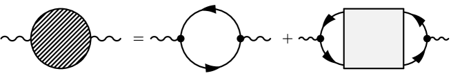
Figure 6: The complete non-equilibrium photon polarization tensor at lowest order in $e$ in terms of the full in-medium two-point function $D_{\psi}$ (lines) and amputated four-point function $\Gamma^{(4)}$ (grey box) in a general theory with charged fermionic fields (for a theory with charged scalar fields there would be an additional tadpole-like contribution).

the full in-medium fermion propagator, and the second term is the contribution from the amputated four-point function $\Gamma^{(4)}$ (see Eq. (131) below), which is represented by the grey box in Fig. 6. In Eq. (127) above, we have defined the “vertex” function

$${\cal V}^{\mu}_{\alpha\beta}(x;u,v)\equiv\Big{(}D_{\psi}(u,x)\,\gamma^{\mu}\,D_{\psi}(x,v)\Big{)}_{\alpha\beta}\,,$$ (129)

where $\alpha$ and $\beta$ denote Dirac indices, and we have introduced the notation

$${\cal V}^{\mu}(x):\Gamma^{(4)}:{\cal V}^{\nu}(y)\equiv\int_{\cal S}{\rm d}u\,{\rm d}\bar{u}\,{\rm d}v\,{\rm d}\bar{v}\,\,{\cal V}^{\mu}_{\alpha\bar{\alpha}}(x;u,\bar{u})\,\Gamma^{(4)}_{\alpha\bar{\alpha};\beta\bar{\beta}}(u,\bar{u};v,\bar{v})\,{\cal V}^{\nu}_{\beta\bar{\beta}}(y;v,\bar{v})\,,$$ (130)

where a sum over repeated Dirac indices is implied. Here, $\Gamma^{(4)}$ denotes the connected four-point function amputated from its external legs:

$$\Big{<}T_{\cal S}\Big{\{}\psi_{\rm s}(x_{1})\bar{\psi}_{\rm s}(x_{2})\psi_{\rm s}(x_{3})\bar{\psi}_{\rm s}(x_{4})\Big{\}}\Big{>}_{\rm s}=-\Delta(x_{1},x_{2}):\Gamma^{(4)}:\Delta(x_{3},x_{4})\,,$$ (131)

where we introduced the “two-particle” function

$$\Delta(u,\bar{u};v,\bar{v})=D_{\psi}(u,\bar{v})\,D_{\psi}(v,\bar{u})$$ (132)

and where we employed a similar notation as before:

$$\Delta(x_{1},x_{2}):\Gamma^{(4)}:\Delta(x_{3},x_{4})\equiv\int_{\cal S}{\rm d}u\,{\rm d}\bar{u}\,{\rm d}v\,{\rm d}\bar{v}\,\,\Delta(x_{1},x_{2};u,\bar{u})\,\Gamma^{(4)}(u,\bar{u};v,\bar{v})\,\Delta(v,\bar{v},x_{3},x_{4})\,.$$ (133)

In order to illustrate how the 2PI effective action formalism might be used to compute the amputated four-point function, we consider the example of a purely fermionic theory with classical action:

$${\cal A}[\psi,\bar{\psi}]=\int{\rm d}^{4}x\Big{(}\bar{\psi}(x)[i\partial\,\!\!\!\!/\,-M]\psi(x)+V(\psi,\bar{\psi})\Big{)}\,$$ (134)

For the relevant case of a vanishing fermionic “background” field, the corresponding 2PI effective action $\Gamma$ can be written as [59, 51]:

$$\Gamma[D_{\psi}]=-i{\rm Tr}\ln D_{\psi}^{-1}-i{\rm Tr}\,D_{0}^{-1}D_{\psi}+\Gamma_{2}[D_{\psi}]+{\rm const}\,,$$ (135)

where the inverse classical propagator is given by

$$iD_{0}^{-1}(x,y)=(i\partial\,\!\!\!\!/\,\!_{x}-M)\,\delta_{\cal S}(x-y)\,.$$ (136)

The exact expression for the functional $\Gamma_{2}[D_{\psi}]$ contains all 2PI diagrams with vertices described by $V(\psi,\bar{\psi})$ and propagator lines associated to the full fermion propagator $D_{\psi}$. The functional trace ${\rm Tr}$ includes an integration over the closed time path ${\cal S}$ as well as integration over spatial coordinates and summation over Dirac indices. In absence of external sources, the equation of motion for $D_{\psi}$ is obtained by minimizing the effective action:

$$\frac{\delta\Gamma[D_{\psi}]}{\delta D_{\psi}(x,y)}=0\,,$$ (137)

which leads to the following Schwinger-Dyson equation for the two-point function:

$$D_{\psi}^{-1}(x,y)=D_{0}^{-1}(x,y)-\Sigma_{\psi}(x,y;D_{\psi})\,,$$ (138)

with proper self-energy given by:

$$\Sigma_{\psi}(x,y;D_{\psi})=-i\frac{\delta\Gamma_{2}[D_{\psi}]}{\delta D_{\psi}(y,x)}\,.$$ (139)

Higher correlation functions can be obtained from appropriate functional derivatives of the 2PI effective action, which generically leads to integral equations. For instance, one can show that the amputated four-point function satisfies the following Bethe-Salpeter equation [58] (space-time variables and Dirac indices are implicit):

$$\Gamma^{(4)}=\Lambda+\Lambda:\Delta:\Gamma^{(4)}$$ (140)

with kernel given by:

$$\Lambda(u,v;\bar{u},\bar{v})=-i\frac{\delta^{2}\Gamma_{2}[D_{\psi}]}{\delta D_{\psi}(u,v)\,\delta D_{\psi}(\bar{u},\bar{v})}\,.$$ (141)

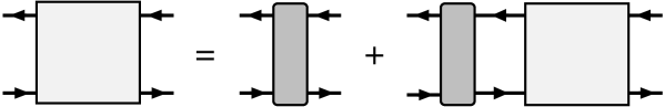
Figure 7: The Bethe-Salpeter equation for the four-point function $\Gamma^{(4)}$ (grey box) in a theory with quartic interactions. The lines represent the full propagator of the theory ($D_{\psi}$) and the dark grey box corresponds to the kernel $\Lambda$ of this integral equation (see text).

Equation (140) is represented graphically on Fig. 7, where the light and dark grey boxes represent the four-point function $\Gamma^{(4)}$ and the kernel $\Lambda$ respectively. This integral equation generates an infinite resummation of ladder graphs with rungs given by the kernel (141). Thus we see that a finite-order truncation of the 2PI effective action in a given expansion scheme automatically leads to an infinite (ladder-type) resummation for the four-point function through Eq. (140). These resummations correspond to the physics of multiple scatterings and actually generalize the gluon ladder resummation recently employed in the context of equilibrium QCD at high temperature to describe the LPM effect [12, 13]. To make this last point more transparent, let us introduce the following resummed vertex function (see Fig. 8):

$$V^{\mu}(x;u,v)\equiv\gamma^{\mu}\,\delta_{\cal S}(x-u)\delta_{\cal S}(x-v)+\Gamma^{(4)}(u,v):{\cal V}^{\mu}(x)\,,$$ (142)

in terms of which the photon polarization tensor can be rewritten (see Fig. 9):

$$\Pi^{\mu\nu}(x,y)=-e^{2}\,{\cal V}^{\mu}(x):V^{\nu}(y)\,.$$ (143)

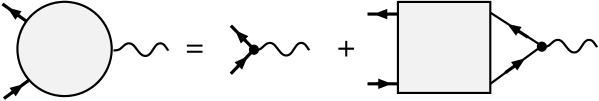
Figure 8: Definition of the resummed vertex $V^{\mu}$ (grey circle) in terms of the bare vertex ($\gamma^{\mu}$) and the amputated four-point function $\Gamma^{(4)}$ (grey square).

Using equation (140), it is now easy to show that the resummed vertex (142) satisfies the following integral equation (space-time variables and Dirac indices are implicit):

$$V^{\mu}=\gamma^{\mu}+\Lambda:\Delta:V^{\mu}$$ (144)

which is graphically depicted on Fig. 10. This, together with Eq. (143) for the photon polarization tensor is a direct generalization of the type of integral equation introduced in Refs. [12, 13] to account for the LPM effect in equilibrium QCD. One can easily convince oneself that the resummation of one-gluon rungs needed there would simply correspond to a two-loop approximation of the corresponding 2PI effective action. It is remarkable that the infinite set of contributions needed to obtain the full photon and dilepton production rates at leading order in $\alpha_{s}$ actually correspond to a finite, ${\cal O}(\alpha_{s})$, truncation of the 2PI effective action.

Figure 9: The non-equilibrium photon polarization tensor $\Pi^{\mu\nu}$ expressed in terms of the resummed vertex $V^{\mu}$ (grey circle).

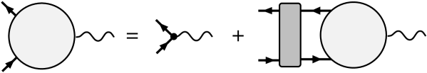
Figure 10: The integral equation satisfied by the resummed vertex $V^{\mu}$ (grey circle). The dark grey box represents the kernel $\Lambda$. This equation resums an infinite series of ladder graphs with rungs corresponding to $\Lambda$.