MCTP-03-42
hep-ph/0310042
September 2003
as a Probe of at the Tevatron
G.L. Kane, Christopher Kolda
and Jason E. Lennon
Michigan Center for Theoretical Physics, University of Michigan,
Ann Arbor, MI 48109, USA
Department of Physics, University of Notre Dame,
Notre Dame, IN 46556, USA
Recently it has been understood that flavor-changing processes mediated by Higgs bosons could be a new and powerful tool for discovering supersymmetry. In this paper we show that they may also provide an important method for constraining the parameters of the minimal supersymmetric standard model (MSSM). Specifically, we show that observation of at the Tevatron implies a significant, model-independent lower bound on in the MSSM. This is very important because enters crucially in predictions and interpretations of the MSSM, though it is difficult to measure. Within specific models, or with other data, the bound becomes significantly stronger.
Over the next several years, the Tevatron at Fermilab will be searching for signs of physics beyond the Standard Model (SM), by directly producing and observing new particles, and by observing rare processes at rates inconsistent with SM predictions. In the latter category falls the search for the rare flavor-changing neutral current (FCNC) decay . Observation of this decay at the Tevatron would necessarily imply new physics since the predicted rate for this process in the SM is far below the search capabilities of the machine. However, supersymmetry (SUSY) naturally predicts large enhancements in the decay rate mediated by neutral Higgs bosons [1, 2, 3, 4], and in some cases yields branching ratios three orders of magnitude above the SM. So observation of the decay would be strong, albeit indirect, evidence in favor of SUSY.
But observation of actually tells us more. We will show that it is possible to deduce bounds on the fundamental SUSY parameter , the ratio of the two Higgs expectation values, from a signal. This is particularly important because is very difficult to measure — there is no general technique for measuring it at hadron colliders — yet almost all SUSY observables depend on it. And a lower limit may be almost as useful as an actual measurement because many SUSY observables quickly saturate as increases. But we can obtain a limit precisely because the rate for does not saturate. Instead it is strongly dependent on , rising (and falling) as . As a secondary feature, we will also be able to obtain some information on the mass scale of the new SUSY Higgs bosons, since the branching ratio scales as the fourth power of their masses.
We will begin by considering two very general scenarios in which all flavor mixing does/does not come from the CKM matrix and in each case we will arrive at a very strong bound. But we will also consider some specific models of SUSY breaking and show that even more stringent bounds can be obtained for these. Our focus will remain on the Tevatron because it has especially good sensitivity to the signal even if it does not reach its full luminosity potential. However the B-factories and LHC can also use this, and related processes, to further probe and the Higgs sector. Unfortunately, if a signal is not seen, non-observation cannot be used to draw absolute conclusions about the parameter space of the MSSM other than to rule out specific model points. It is always possible to choose SUSY parameters in such a way to push the signal down to the level of the Standard Model where it would not be observed.
1 Higgs-Mediated
First, a little theoretical background. The question of flavor-changing neutral currents (FCNCs) mediated by Higgs bosons was first addressed two decades ago by Glashow and Weinberg [5]. It had always been obvious that the Higgs boson of the minimal standard model could not have flavor-violating couplings since the couplings of fermions to the Higgs field defines the fermion mass eigenstates and thus also defines our notion of flavor. But in models with two (or more) Higgs fields, the fermion mass eigenbasis can be different from the Higgs interaction eigenbasis and thus Higgs-mediated FCNCs can occur. In order to avoid large FCNCs inconsistent with experiment, the authors of Ref. [5] proposed several solutions. One of those solutions is the “type II” two-Higgs-doublet model: one Higgs field () couples only to up-type quarks, while the other () couples only to the down-type: . This guarantees the alignment of the Higgs boson interaction eigenbasis with the fermion mass eigenbasis. Such a structure can be protected from quantum corrections by any number of discrete symmetries under which the two Higgs fields transform differently.
The MSSM possesses the structure of a type-II model classically. But it possesses no discrete symmetry which can protect this structure; all such symmetries are broken by the -term in the superpotential, which must be present to avoid disagreement with experiment. And though the type-II structure is also protected by holomorphy of the superpotential, this too is ineffective after SUSY is broken. Thus new terms are generated in the low-energy Lagrangian of the MSSM of the form . Whether such terms will lead immediately to FCNCs depends on the structure of the new Yukawa matrices [1, 2, 3, 4].
In Ref. [1] it was shown that there are contributions to which are flavor-violating and can have important effects at large . It is actually quite easy to see why. Consider the diagram in Fig. 1(a) in which charged higgsinos propagate inside the loop. If we work in a basis in which the down quarks couple diagonally to , then the up quarks have off-diagonal couplings to proportional to CKM elements. In particular, the coupling of to is just the bottom Yukawa coupling, . But the coupling of to is then where is the top-quark Yukawa coupling. Thus the diagram generates a new interaction with coefficient proportional to . We can rewrite this coefficient as simply , where includes not only but also the loop kinematic and suppression factors. (We ignore the phases induced by the sparticles in the loops; work including them is under way [6].)

When gets a vev (), it contributes an off-diagonal piece to the fermion mass matrix:
| (1) |
This Lagrangian is written in the Higgs interaction eigenbasis of the fermions, which at tree-level is also the mass eigenbasis; we drop the first generation for simplicity. The mass matrix can be diagonalized by a biunitary transformation which mixes the and by an angle . But since , we have . So although is one-loop suppressed, the factor of can allow to be .
At tree-level, a Higgs transition is possible, with the Higgs decaying to leptons, as in Fig. 2. This occurs by exchange of . However the coupling of the -quark sector to has shifted the -quark interaction eigenstates away from their mass eigenstates. In order to replace the interaction eigenstates on the external legs with mass eigenstates, we must replace
| (2) |
which induces a transition through an Higgs, Fig. 2. Then the flavor-changing amplitude is related to the flavor conserving amplitude by
| (3) |
There are several noteworthy properties of the Higgs-mediated FCNCs. First, the amplitude for scales as at large . One factor of come from , the other two come from the - and -Yukawa couplings which scale as . Thus the branching ratio scales as and provides an incredibly powerful tool for constraining . Second, at large , the Higgs doublet is essentially decoupled from the electroweak symmetry breaking. It contains the physical states , and which all have roughly equal masses. But because Higgs flavor changing must disappear in a model with only one Higgs doublet, the FCNC branching ratios must decouple as . But this does not mean that the effects decouple as the SUSY mass scale increases. Rather, in the limit that all supersymmetric masses are taken heavy, while (or ) remains light, the rate for Higgs FCNCs approachs a finite constant.
What diagrams contribute to the off-diagonal Higgs couplings? First, even if all flavor violation stems from the CKM matrix alone, there is the one-loop higgsino diagram of Fig. 1(a) already considered. Models with only this CKM-induced flavor violation are known as “minimal flavor violation” (MFV) models. Note that this kind of flavor violation has nothing to do with the “SUSY flavor problem.” It is always present in SUSY because it is generated by the flavor violation in the CKM matrix and cannot be eliminated simply by making superpartners heavy or by aligning quark/squark mass matrices.

More generally there are also gluino loop diagrams contributing to the same interactions (Figure 1(b)), if flavor-violating or squark mass insertions are non-zero. Such an insertion can be generated in minimal models by renormalization group running of the squark mass matrices, or may appear in the underlying theory. We make no assumptions in our general analysis about the underlying source of this flavor-changing in the squark sector, and we refer to this as general flavor violation.
Because this new source of FCNCs emerges from the Higgs sector, it preferentially generates processes involving heavy fermions. Thus the channels in which Higgs-mediated FCNCs can most easily be observed are and . The channels with final state muons are suppressed relative to those with final state taus by but are much cleaner experimentally. The channels with initial state are suppressed relative to by . Thus a machine which produces an abundance of and can cleanly tag and measure muons is ideal for studying this physics. This machine is precisely the Tevatron, either in CDF or D0. The current limits on are provided by CDF from Run I at and respectively. Given enough luminosity, the -factories may be able to corroborate any Tevatron discovery using or, if a suitable technique is found, .
If CDF and D0 each record even of data during Run II of the Tevatron, now underway, they can probe the branching fraction below the level. (See, e.g., Ref. [8] for a more detailed study of the CDF capabilities.) We will for illustration assume that the Tevatron can discover a signal in if its branching ratio is greater than . Because the branching ratios scale as high powers of the input parameters ( and ), small changes in the Tevatron capabilities will generate infinitessimal changes in our results. And once a signal is discovered, the numerical analysis can be redone to obtain more precise limits.
We demonstrate below that there is a minimum value of consistent with a signal at the level, and calculate it. We also consider the interplay between the pseudoscalar mass and , a result which could be important in searches for the additional Higgs bosons at future colliders. Both of these analyses will be done in full generality within the MSSM. We will not constrain ourselves initially to any particular class of MSSM models, such as supergravity- or anomaly-mediated SUSY-breaking. This can be done because there are only a limited number of parameters on which the branching ratio will depend and these few parameters can be studied without further simplifications or assumptions. However in particular classes of models the constraints on and are stronger and therefore observation of a signal provides even more information. We will consider specific SUSY models after doing the general analysis and we will find bounds on much stronger than in the general case.
2 Minimal Flavor Violation: Higgsino Contribution
Regardless of any details of SUSY-breaking, the higgsino contribution of Fig. 1(a) to Higgs-mediated flavor-changing processes must be present. First we will consider the case where only this contribution is present and then generalize in the next section. Thus we begin by considering the MFV models.
The flavor-changing contribution of the higgsino loop diagram is encoded in a new dimensionless parameter such that
| (4) |
Here is the QCD correction due to running between the SUSY and scales, and we take . Note that the fraction approaches at large .
The parameter is calculated to be [1]
| (5) |
where and are the left- and right-handed top squark masses, is the superpotential Higgs mass parameter, is the top-squark trilinear term, and the function is defined in Ref. [1]. The important thing to know about is that it is positive definite, symmetric in its inputs and up to a constant of . In particular, and .
In order to maximize the function (and therefore maximize the branching fraction one can obtain for a given ) we need only consider the four parameters , , and . This is easiest to do by considering the limits in which could become large.
First consider the limit in which is much larger than the squark masses. Then since appears both in and as a prefactor. Thus it appears that can grow unabated as becomes large. Such a runaway behavior would generate arbitrarily large branching ratios and invalidate our claim to a bound on . However, there is a “cosmological” limit to : as increases far beyond the squark masses, the usual electroweak vacuum become unstable with the true vacuum breaking QED and QCD [9]. We apply this constraint by applying the famous condition
| (6) |
(The last term, , is the mass parameter for appearing in the Higgs potential. Since is necessary to break the electroweak symmetry, we can maximize by setting .) Because the squark masses are much smaller than in this limit, then can not become much larger than unity at best. A similar argument holds for large but with smaller than the squark masses, except now is more highly suppressed, .
The actual limit is obtained when becomes large along with one of the squark masses (with the other as small as possible). Then . But the QED/QCD-breaking constraint still limits , though now it becomes so that which implies that
| (7) |
Plugging into Eq. (4) immediately gives
| (8) |
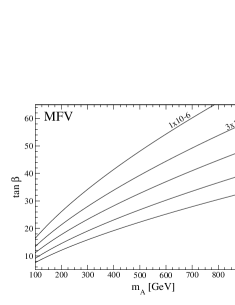
Thus for (approximately its current lower limit) and a branching ratio greater than , we deduce in an MFV scenario that . As increases, the bound on also increases rapidly; for example, if , one must have . In general,
| (9) |
where we have taken for large .
In Figure 3, we plot contours representing the maximal value of the branching ratio consistent with a given choice of and . Given a measured value of the branching ratio, only the region above the line is consistent in an MFV scenario.
3 General Flavor Violation: Gluino Contributions
In the case of MFV, only the higgsino loop has any significant effect in producing flavor violation. However once one moves away from truly minimal flavor violation, a new source arises. In a truly general scenario, the -- couplings can be flavor changing. In the mass insertion approximation, these violations are moved to the squark propagators where they appear as bilinear interactions which mix flavors and even chiralities of the squarks. The size of the insertions is parametrized by a dimensionless quantity, where are either or , and label the squark generation. We are only interested in the down-sector and insertions for this work. At present there are no strong experimental bounds on these insertions and so it is possible that the and (or and ) are maximimally mixed, or . Of course, in particular models a large could lead to large or , but constraints from these processes are sensitive to while is sensitive to alone. Since we allow very large flavor-mixing, we must take care to note that the mass insertion approximation breaks down as approaches one; we will discuss this issue shortly.
The new gluino-induced source of flavor changing in general models generates new diagrams in with and squarks and gluinos in the loop; see Fig. 1(b). For our purposes here we can ignore the higgsino contributions since their maximal size is smaller than that of the gluino loop if . We will also assume that only one of the two diagrams in Fig. 1(b) dominates the branching ratio; when there is data, a fully combined analysis should be done. Specifically we will choose the diagram to dominate, though our results are identical if the diagram dominates instead. We will discuss more realistic scenarios at the end of the section.
We parametrize the gluino contribution as
| (10) |
where the function is defined in Ref. [7]. The branching ratio is calculated from just as for in Eq. (4). Notice in particular the lack of a suppression in ; this will allow much smaller values of to be consistent with an experimental signal.
There are two limits in which we can simplify the above expression. For small – mixing, we can usually take in Eq. (10) and then work in the mass insertion approximation. However, if there is a large hierarchy in between and , or if there is large mixing, that approximation breaks down. Instead, it is far easier to work directly in the basis of the mass eigenstates. Defining as and its orthogonal combination, we must replace the product in Eq. (10) with
| (11) |
The inequality follows only from the positivity of the function . Given more information in the future about the squarks (masses or lower bounds) it may be possible to find a lower bound on the second term and thus an improved upper bound on the branching fraction.
Like the MFV case there is a possible runaway behavior in computing the diagrams in Fig. 1(b), allowing for arbitrarily large branching ratios. In the MFV case, this arose as , which we cut off by demanding that color-breaking minima deeper than the SM minimum not appear. In a general case, this arises as for which the color-breaking constraint is useless. However there are equally powerful constraints which rely on fine-tuning arguments, which have recently been strengthened [12]. In particular, the -parameter appears in the Higgs potential and it is the minimization of this potential which must supply the weak scale. There is a well-known relation among the -term and other Higgs soft mass terms which must together generate the scale :
| (12) |
If then a fine-tuning must be arranged among , and in order to generate on the left hand side of the Eq. (12). We will require , which is a statement that we allow less fine-tuning in the electroweak potential than about one part in 60. However in our expressions we will show how to scale our results for other choices of , in case the reader wishes to apply their own fine-tuning constraint.
In order to calculate the upper bound on the branching ratio, it is useful to note that the product reaches its upper bound when the squarks are as light as possible and degenerate, and . Then one can derive the semi-analytic bound (assuming maximal mixing):
| (13) |
leading to
| (14) |
and
| (15) |
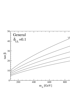
Contours of the maximum allowed branching ratio are plotted in Fig. 4 as a function of and for the case of maximal mixing. For small mixing we can return to the mass insertion approximation in which case
| (16) |
The bounds presented in this section should be considered the absolute limits on given a signal at the Tevatron at the level. Nowhere did we inject theoretical constraints stemming from some particular model of SUSY. On the other hand, if we had a model, or other information, we could devise much stronger bounds. For example, many observables in SUSY depend on , so that once SUSY is found, we will very quickly have constraints on , which would allow more precise bounds. And if we have some theoretical or experimental reason to believe in a particular model of SUSY-breaking, then we know even more. As we will discuss in Section 4, models produce bounds which are much stronger than the general case.
3.1 “Nearly-Minimal” Flavor Violation
For most purposes, the bounds in the previous section are too general. SUSY models which are truly generic and general have an embarassing wealth of flavor-changing mass insertions like . Most of these insertions must be miniscule in order to avoid dangerously large FCNCs in well-studied processes, such as - mixing. Thus one usually imposes on SUSY some form of organizing principle which prevents most of these insertions from becoming large, whether that be mass degeneracies or mass matrix alignment.
However even in models which naturally solve the SUSY flavor problem, one usually still expects some flavor violation to reappear by way of renormalization effects. The most common source of these is the presence of the up-quarks Yukawa matrix in the renormalization group equations for the left-handed squarks. Because all Yukawa matrices cannot be simultaneously diagonalized, non-zero will be generated. (The mass insertions will not be generated at leading order.) However there is a significant difference between these mass insertions and those considered in the general case above: here will be proportional to the corresponding element of the CKM matrix. For example, will be naturally suppressed by . Thus one typically finds which in turn would force for . However this bound is not a true limit – the model can be tuned in order to obtain the same branching ratio but with much smaller values of .
Thus, while one expects from theoretical arguments that must be greater than 9 in order to see a signal at the Tevatron, the true mathematical limit remains at as found in the previous section, until the origins of SUSY flavor physics are better understood.
3.2 Relation to Other Observables
The bound on in the general case depends strongly on the (or ) mixing present in the strange–bottom squark sector. But there are several other key observables which also depend on this mixing and which should be measured or constrained over the next few years. Key among them are – mixing, parametrized by , and the rate and CP asymmetry in . On the subject of , we will not say very much, but refer the reader to Ref. [13] for a full discussion.
The situation for is more interesting. In the presence of a single, dominating (or ) mass insertion, a calculation of yields the approximate formula:
| (17) |
where is roughly 15 to . The same formula also holds with the substitution . (To obtain this simple result, we have followed the calculations of Ref. [15] for – mixing, appropriately modified, and assumed all squark and gluino masses are essentially degenerate at .) Since can be complex, the SUSY contributions can either add to or subtract from the SM prediction for . A measurement of near its SM value would indicate either large or small , either one of which would suppress and thus tighten our bound on . Once SUSY partners are discovered, the value of will be known and a very stringent bound on can be extracted from the data, strengthening our bound on further.
4 Supersymmetric Models
In the previous sections, we performed very general analyses in determining what could be learned about the SUSY parameter space by measuring . Now we ask the same question, but in the context of specific models of SUSY-breaking, namely the three most commonly studied models: minimal supergravity models (mSUGRA, also called the constrained MSSM), minimal gauge-mediated (GMSB) models, and minimal anomaly-mediated (AMSB) models. Realistic models will necessarily yield much stronger bounds on and for two reasons: first, there is no reason for their contributions to FCNCs to be maximal, and second there are often correlations with other processes which suppress the flavor-changing contributions. Several analyses of in the context of SUSY models have been completed [10] and a more detailed study of this will appear shortly [14]; here we summarize some of the important results of this last study. Namely we will find bounds on in specific models for an observed and discuss their implications.
For each of the three models to be discussed, we will vary all the free parameters of the models and at each “model point” calculate the branching fraction [11]. However we will also apply several phenomenological constraints to avoid points which are unphysical. The most important constraints come from the muon magnetic moment [16] and the transition [17]. For the former, we will demand that the SUSY constributions to fall between and . For the latter, we will demand that calculated rate for fall between and . In both cases these are rather wide windows. For the muon magnetic moment, a wide window is required by the inconsistency of the and data sets which are used to calculate the standard model hadronic contributions to . For we use a wide window because of the uncertainties in the next-to-leading order calculation of the SUSY contributions.
4.1 Minimal supergravity
Minimal supergravity (mSUGRA) actually contributes fairly efficiently to Higgs-mediated FCNCs. It has three key ingredients that help to generate large branching ratios. First, mSUGRA models often have large trilinear terms, necessary for the higgsino contribution. Second, the extended running from the GUT scale down to the weak scale generates considerable mixing between the second and third generation squarks, allowing for a sizable gluino contribution. Finally, the pseudoscalar Higgs does not come out particularly heavy.
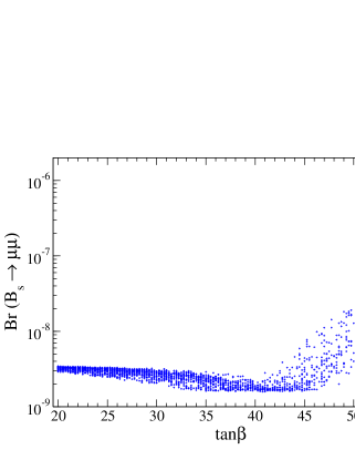
In Fig. 5(a), we show a scatter plot of points in the mSUGRA model space, each one representing a distinct choice of , , , and (we take only), consistent with all experimental and theoretical constraints. There are several important lessons to draw from the figure. One should immediately note that mSUGRA models exist, consistent with all other constraints, that have rates for right up to the CDF bound; in fact, models were found that passed all other constraints, except the bound, indicating that is already a non-trivial constraint on mSUGRA models.

We also notice that mSUGRA models with a branching ratio greater than require . Thus observation of at Run II would certainly indicate very large if mSUGRA is the correct model.
One also notices another interesting feature in the figure, namely a bifurcation of the points at the largest branching fractions. The points in the upper arm all have while all the points with lie in the main body of points. This behavior is rooted in the constraint. For , models with very large also have chargino contributions to which tend to cancel the SM. Thus the resulting is too small and we throw the model point out. As the SUSY mass scales increase, the cancellation goes away, but the rate for is also suppressed. However, the cases with exhibit a very different behavior. For light spectra, these models can have SUSY contributions to much larger than those of the SM, but with opposite sign, so that after adding the two pieces, the resulting rate is still roughly consistent with the SM and with experiment. Then as the SUSY mass scale is increased, the two pieces start to cancel to zero, ruling out the model points. As the SUSY scale is further increased, the SUSY contribution decouples and the SM once again dominates. Thus a gap is generated where the models predict .
Thus models with can only be observed in Run II if while models with can have down to 40. The upshot of this is that a measurement of and an independent measurement of could indicate that . However, these measurements alone cannot be used to show that .
4.2 Anomaly Mediation
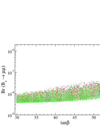
The simplest models with pure anomaly mediation have only one free parameter, an overall mass scale, but are not phenomenologically viable. But one can define a “minimal” anomaly-mediated model which has two free parameters: an overall mass scale for the anomaly mediation, and a separate mass scale just for the scalars. We considered this minimal model, by varying both of these parameters, as well as , and studying the resulting spectra. In principle, AMSB shares many of the same features that make mSUGRA a nice candidate for discovery of . In practice, this is only partially true. In AMSB the constraint is much stronger and rules out many model points where a large Higgs-mediated FCNC signal would have been predicted. We do not find any models with observable branching fractions of into muons , consistent with the result of Baek et al. [10]. However, we note that this result depends very strongly on the calculation; changes in the NLO calculation could easily allow for much larger (or smaller) branching fractions.
A scatter plot of the allowed parameter space is shown in Fig. 6(a). This figure again shows a bifurcation into two separate regions, though this time much more distinct than in the mSUGRA case. Here there is no fundamental difference between the two regions, but the basic explanation is similar to the case of the last section. For AMSB models with large and intermediate masses, the SUSY contribution to tends to cancel the SM, predicting a rate which is too small. For large masses, the SUSY contribution decouples, but then so does . However, there is a region of very light masses where the SUSY contribution is roughly twice the SM contribution, but with opposite sign, so that their sum squared is consistent with data. This last region is the upper-right region of the figure. There we see that one can have are large as only if .
4.3 Gauge Mediation
Unlike the previous two cases, one would not expect a large Higgs-mediated FCNC signal in models with gauge mediation. Whereas mSUGRA has a large and lots of running to generate squark mixing, gauge-mediated models have neither. At the mediation scale, (so no higgsino contribution) and there is little running unless the mediation scale is large (so no gluino contribution). Indeed, we find that it is very difficult to generate observable signals at the Tevatron for GMSB models, even without invoking constraints from . This is best summarized by Fig. 7, where no models are found with above , making this signal difficult if not impossible to observe in Run II.
To obtain this figure, we varied all the parameters of the GMSB model, including the number of messengers, which we allowed to take values of , 3, and 5. We also allowed the messenger scale, , to go as high as . At such large , one would expect to maximize your signal since both -terms and squark mixing benefit from the running between and . And indeed the maximum signals are occurring for large messenger scales. However even with such a large scale, there is little signal in this channel compared to mSUGRA or AMSB models. Thus a signal at the Tevatron tells us something significant that has nothing to do with — it would be evidence against gauge mediation itself [10, 14]!
5 Conclusions
Over the next several years, the Tevatron’s physics program has a strong opportunity to discover new physics in the rare decay . And if either CDF or DØ do observe this signature, they will have simultaneously provided very strong evidence for a supersymmetric world just beyond our current reach. And they will have provided an important insight into SUSY-breaking and its mediation mechanism. And they will have placed a lower bound on the parameter , vitally important to future studies of SUSY. It is the existence of this lower bound, and its value, that we have derived in this work.
The SUSY parameter is one of the most important quantities which needs to be measured in a supersymmetric world. In a top-down approach, the calculation of from first principles would be an important test of some underlying theory. In a bottom-up approach, is a necessary input to the Yukawa sector and thus relevant to everything from Yukawa unification to radiative electroweak symmetry breaking. Almost all predictions that can test the form of the underlying theory depend on in some way, so it must be measured as a first step in studying and testing models of SUSY. Yet is infamously difficult to measure, particularly at hadron colliders or in rare decays — all methods proposed to date are model and/or parameter dependent.
The decay may improve the situation dramatically because it is unusually sensitive to , providing an opportunity to bound if a signal is seen. In this paper we showed that some very general theoretical assumptions that do not depend on specific models allow us to put significant lower bounds on given a signal. In the general case with large flavor changing effects allowed (), the bound is given by Eq. (15), leading to . This bound increases quickly with decreasing flavor violation: for the bound is pushed to (Eq. (16)). In more typical models in which or , then if a signal is seen at the Tevatron. However, the decay does not require new sources of flavor changing to be present; it can be induced simply from the flavor changing already present in the standard model CKM matrix. In such a case a stronger bound is obtained (Eq. (9)). These bounds are for a ; we have also shown how to scale the bounds as a function of the branching fraction. Finally, we find that the bounds are significantly stronger in often studied models such as minimal supergravity.
For many purposes, a lower limit is as good as a measurement since many observables (, , dark matter signals, etc) saturate as increases. There is also an upper limit on of order 60 from the requirement that the theory remain perturbative up to high (unificiation) scales. Thus a lower limit often is tantamount to a measurement.
Acknowledgements
We are grateful to K. Hidaka for helpful comments on the manuscript. This work was supported in part by the National Science Foundation under grant PHY00-98791 and by the U.S. Department of Energy under grant DE-FG02-95ER40896.
References
- [1] K. S. Babu and C. Kolda, Phys. Rev. Lett. 84, 228 (2000).
-
[2]
C. S. Huang, W. Liao and Q. S. Yan,
Phys. Rev. D 59, 011701 (1999);
C. Hamzaoui, M. Pospelov and M. Toharia, Phys. Rev. D 59, 095005 (1999);
S. R. Choudhury and N. Gaur, Phys. Lett. B 451, 86 (1999);
C. S. Huang, W. Liao, Q. S. Yan and S. H. Zhu, Phys. Rev. D 63, 114021 (2001). -
[3]
C. S. Huang and W. Liao,
Phys. Lett. B 525, 107 (2002) and
Phys. Lett. B 538, 301 (2002);
C. Bobeth, T. Ewerth, F. Kruger and J. Urban, Phys. Rev. D 64, 074014 (2001) and Phys. Rev. D 66, 074021 (2002);
A. J. Buras, P. H. Chankowski, J. Rosiek and L. Slawianowska, Nucl. Phys. B 619, 434 (2001), Phys. Lett. B 546, 96 (2002) and Nucl. Phys. B 659, 3 (2003);
G. Isidori and A. Retico, JHEP 0111, 001 (2001) and JHEP 0209, 063 (2002). - [4] A. Dedes, arXiv:hep-ph/0309233.
- [5] S. L. Glashow and S. Weinberg, Phys. Rev. D 15, 1958 (1977).
- [6] K. Hidaka, G.L. Kane and C. Kolda, in preparation.
- [7] K. S. Babu and C. Kolda, Phys. Rev. Lett. 89, 241802 (2002).
- [8] R. Arnowitt, B. Dutta, T. Kamon and M. Tanaka, Phys. Lett. B 538, 121 (2002).
- [9] J. F. Gunion, H. E. Haber and M. Sher, Nucl. Phys. B 306, 1 (1988).
-
[10]
A. Dedes, H. K. Dreiner and U. Nierste,
Phys. Rev. Lett. 87, 251804 (2001);
R. Arnowitt, B. Dutta, T. Kamon and M. Tanaka, Phys. Lett. B 538, 121 (2002);
S. Baek, P. Ko and W. Y. Song, Phys. Rev. Lett. 89, 271801 (2002) and JHEP 0303, 054 (2003);
H. Baer et al., JHEP 0207, 050 (2002);
A. Dedes, H. K. Dreiner, U. Nierste and P. Richardson, arXiv:hep-ph/0207026;
J. K. Mizukoshi, X. Tata and Y. Wang, Phys. Rev. D 66, 115003 (2002);
T. Blazek, S. F. King and J. K. Parry, arXiv:hep-ph/0308068. -
[11]
Model points were generated using the package SOFTSUSY:
B. C. Allanach, Comput. Phys. Commun. 143, 305 (2002) [arXiv:hep-ph/0104145]. - [12] G. L. Kane, J. Lykken, B. D. Nelson and L. T. Wang, Phys. Lett. B 551, 146 (2003).
- [13] G. L. Kane, P. Ko, H. B. Wang, C. Kolda, J. H. Park and L. T. Wang, arXiv:hep-ph/0212092 and Phys. Rev. Lett. 90, 141803 (2003).
- [14] C. Kolda and J. Lennon, in preparation.
-
[15]
D. Becirevic et al.,
Nucl. Phys. B 634, 105 (2002);
P. Ko, J. Park and G. Kramer, Eur. Phys. J. C 25, 615 (2002). -
[16]
The experimental constraints on are based on:
G. W. Bennett et al. [Muon g-2 Collaboration], Phys. Rev. Lett. 89, 101804 (2002).
For theoretical constraints in the context of SUSY see, e.g.:
M. Byrne, C. Kolda and J. E. Lennon, Phys. Rev. D 67, 075004 (2003). -
[17]
The experimental constraints on are based on:
K. Abe et al. [Belle Collaboration], Phys. Lett. B 511, 151 (2001);
S. Chen et al. [CLEO Collaboration], Phys. Rev. Lett. 87, 251807 (2001).
For the calculation within SUSY see:
M. Ciuchini, G. Degrassi, P. Gambino and G. F. Giudice, Nucl. Phys. B 534, 3 (1998);
G. Degrassi, P. Gambino and G. F. Giudice, JHEP 0012, 009 (2000);
M. Carena, D. Garcia, U. Nierste and C. E. Wagner, Phys. Lett. B 499, 141 (2001).