SLAC–PUB–10185 November, 2003 hep-ph/0310039

Top Quarks and Electroweak Symmetry Breaking in Little Higgs Models

Maxim Perelstein

Newman Laboratory for Elementary Particle Physics,
Cornell University, Ithaca, NY 14853 USA

and

Michael E. Peskin and Aaron Pierce

Stanford Linear Accelerator Center, Stanford University
2575 Sand Hill Road, Menlo Park, CA 94025 USA

ABSTRACT

‘Little Higgs’ models, in which the Higgs particle arises as a pseudo-Goldstone boson, have a natural mechanism of electroweak symmetry breaking associated with the large value of the top quark Yukawa coupling. The mechanism typically involves a new heavy $SU(2)_{L}$ singlet top quark, $T$. We discuss the relationship of the Higgs boson and the two top quarks. We suggest experimental tests of the Little Higgs mechanism of electroweak symmetry breaking using the production and decay of the $T$ at the Large Hadron Collider.

Submitted to Physical Review D

1 Introduction

The most pressing question in elementary particle physics today is that of identifying the mechanism responsible for the spontaneous breaking of the $SU(2)\times U(1)$ symmetry of the weak interactions. For many years, the list of candidate answers to this question was static. The leading alternatives were supersymmetry and new strong interactions at the TeV scale. Recently, the list has expanded to include several new mechanisms, including candidates gleaned from analyses of models with extra dimensions. Whatever the mechanism of electroweak symmetry breaking, we expect it to be associated with the TeV scale, which we will explore soon at the Large Hadron Collider (LHC). It is important, then, to clarify the implications of these new mechanisms and the observable processes by which they might be tested.

One of the most appealing of the newly proposed approaches to electroweak symmetry breaking is that of the ‘Little Higgs’ [1, 2, 3, 4, 5, 6]. This model revives the idea that the Higgs particle is a pseudo-Goldstone boson [7, 8, 9], adding to it a number of insights from the study of extra dimensions, supersymmetry and other weak-coupling Higgs theories. Proponents of the Little Higgs argue that the large top Yukawa coupling can generate the instability of the Higgs potential to electroweak symmetry breaking. The construction links the observed heaviness of the top quark to electroweak symmetry breaking in a manner different from that in supersymmetry [10, 11, 12, 13] or topcolor [14] models, through a mechanism that is direct and appealing. In this paper, we will discuss the relation between this mechanism and the properties of the top quark and its partners.

Little Higgs models typically contain a large multiplet of pseudo-Goldstone bosons, including the Higgs doublet of the Standard Model. While many of the Goldstone bosons in this multiplet receive masses at the TeV scale, the models are constructed so that the Higgs boson mass is protected from quadratic divergences at the one-loop level. The dominant contributions to the Higgs boson mass parameter are only logarithmically sensitive to the physics at the cutoff and are therefore calculable. The (mass)² parameter generated by gauge interactions in perturbation theory is positive. However, the couplings of the Higgs boson to the top quark and to a new heavy vector-like quark can overcome the positive contribution, and produce total (mass)² parameter for the Higgs doublet that is negative. Therefore, like supersymmetry and topcolor, the explanation of the negative (mass)² of the Higgs boson is tied to its couplings to the top sector. However, there is an advantage that Little Higgs models have with respect to supersymmetry. In supersymmetry, the calculation of electroweak symmetry breaking combines the contribution from the top sector with the independent parameters $\mu$ and B$\mu$, whereas in the Little Higgs model the top contribution stands on its own.

In the Little Higgs model, the couplings of the Higgs to the Standard Model top quark, $t$, and the new heavy top quark, $T$, form an independent sector that is relatively isolated from the rest of the Higgs dynamics. This allows us to make statements about the dynamics of the $T$ that are general in models making use of the Little Higgs mechanism. Tests of these statements test the underlying mechanism of electroweak symmetry breaking.

In this paper, we will consider only models with one new heavy top and one pseudo-Goldstone boson Higgs doublet. Our conclusions are general with these assumptions. More complicated top sectors and models with multiple Higgs doublets have been proposed [15, 16, 17, 18, 19, 20, 21].

The plan of this paper is as follows: In Section 2, we will review the mechanism of electroweak symmetry breaking in Little Higgs models. From this discussion, we will obtain a relation among the parameters of the Lagrangian that couples the Higgs to the top quarks. The rest of our discussion will be concerned with methods of testing this relation. In Section 3, we will discuss the parameters of a simple version of the Little Higgs model and the constraints on these parameters from precision electroweak measurements. This discussion will build on the work of [22, 23, 24]. The goal of this section will be to determine the acceptable values of the $T$ mass. In Section 4, we will discuss the phenomenology of the $T$. We will argue that, though the $T$ is to first order a weak interaction singlet, it decays significantly to $W^{+}b$ and $Z^{0}t$. These modes provide important signatures for $T$ production at the LHC. We will argue that the measurement of the total width of the $T$ and of its production cross section tests the relation highlighted in Section 2. Section 5 presents some conclusions.

Some other aspects of the Little Higgs model collider phenomenology have been discussed in [25, 26, 27].

2 Electroweak symmetry breaking in Little Higgs models

As we have already noted, electroweak symmetry breaking in Little Higgs models can result from coupling the Little Higgs multiplet to an isolated sector containing the top quark and another heavy quark. In this section, we will review this mechanism as it was presented in [3, 4]. We will not be concerned with the entire computation of the Higgs potential, only with the generation of one term in which the Higgs (mass)² is negative. We will see that the mechanism of  [3, 4] is a simple and attractive way to meet that goal. The mechanism involves an additional heavy charge-$\frac{2}{3}$ quark. The idea that a heavy singlet quark mixing with the top quark as a part of electroweak symmetry breaking was originally introduced as the ‘topcolor seesaw’ of Dobrescu and Hill [28]. In the following, we will use the letter $u$ or $U$ to denote weak eigenstates and $t$ or $T$ to denote mass eigenstates. Then, the third-generation weak doublet will be $(u,b)_{L}$, the new left-handed weak singlet will be $U_{L}$, and the two right-handed weak singlets of the model will be $u_{R}$, $U_{R}$. We will identify the $t$ and $T$ states momentarily.

A key feature of the Little Higgs construction is the presence of global symmetries which protect the Higgs boson mass against quadratically divergent radiative corrections at one-loop. The Higgs boson couplings to quarks should preserve this feature. As a demonstration of how this could work, we introduce an $SU(3)$ global symmetry. Let $V$ be an $SU(3)$ unitary matrix, depending on Goldstone boson fields $\pi^{a}$ as

$$V=\exp[2i\pi^{a}t^{a}/f]\ ,$$ (1)

where $f$ is a “pion decay constant” with the dimensions of mass and $t^{a}$ is an $SU(3)$ generator, normalized to ${\mbox{\rm tr}}[t^{a}t^{b}]=\frac{1}{2}\delta^{ab}$. We will identify the Higgs doublet $H\equiv(h+i\pi_{3},\,-\sqrt{2}\pi^{-})^{T}$ with the $SU(2)$ doublet components of the Goldstone boson matrix $\Pi\equiv\pi^{a}t^{a}$:

$$2i\Pi=\frac{1}{\sqrt{2}}\pmatrix{\Phi&H\cr-H^{\dagger}&\phi\cr}.$$ (2)

$\Phi$ and $\phi$ are other members of the Goldstone multiplet that we need not concern ourselves with at this point. Let $\chi_{L}$ be the ‘royal’ $SU(3)$ triplet $(u,b,U)_{L}$ [29]. These fields can be coupled by writing [3, 4]

$$\mathcal{L}=-\lambda_{1}f\,\overline{u}_{R}V_{3i}{\chi_{L}}_{i}-\lambda_{2}f\,\overline{U}_{R}U_{L}+{\rm h.c.}\$$ (3)

The first term of this Lagrangian has an $SU(3)$ global symmetry

$$V_{3i}\to V_{3j}\Lambda^{\dagger}_{ji},\qquad\chi_{L}\to\Lambda\chi_{L}\ .$$ (4)

This symmetry is spontaneously broken. To the extent that this $SU(3)$ is an exact symmetry of the Lagrangian, the Goldstone boson fields, $\pi^{a}$, must remain massless. The second term in (3) explicitly breaks the $SU(3)$ symmetry to $SU(2)$ and specifically breaks the symmetries responsible for keeping $H$ and $H^{\dagger}$ in (2) massless. However, the Higgs boson field does not enter this term directly. This means that $H$ can obtain mass only from loop diagrams, and only at a level at which the couplings $\lambda_{1}$ and $\lambda_{2}$ both enter. In [3], it is shown that this restriction prohibits the appearance of one-loop quadratic divergences in the Higgs boson mass. The one-loop radiative contribution to the Higgs (mass)² is only logarithmically divergent, and can thus be reliably estimated. This contribution turns out to be negative [3], giving an explicit mechanism of electroweak symmetry breaking.

Let us review both aspects of the calculation. We expand about the symmetric point, $\left\langle{h}\right\rangle=0$. At this point, $u_{L}$ remains massless, while $U_{L}$ combines with one linear combination of $u_{R}$ and $U_{R}$ to obtain a mass. The mass eigenstates are then

$$t_{L}=u_{L}, t_{R}={\lambda_{2}u_{R}-\lambda_{1}U_{R}\over\sqrt{\lambda_{1}^{2}+\lambda_{2}^{2}}},$$

$$T_{L}=U_{L}, T_{R}={\lambda_{1}u_{R}+\lambda_{2}U_{R}\over\sqrt{\lambda_{1}^{2}+\lambda_{2}^{2}}},$$ (5)

with $m_{t}$ massless at this level and

$$m_{T}=\sqrt{\lambda_{1}^{2}+\lambda_{2}^{2}}\,f.$$ (6)

The Feynman rules for couplings between the Higgs boson and the top quarks in the symmetric vacuum are given in Fig. 1. We only show rules involving one or two Higgs bosons, which are relevant to the calculation of the one-loop quadratic divergence. The couplings of the Higgs boson to $t_{L}\overline{t}_{R}$ and to $t_{L}\overline{T}_{R}$ are related to the parameters appearing in the Lagrangian (3) via

$$\lambda_{t}={\lambda_{1}\lambda_{2}\over\sqrt{\lambda_{1}^{2}+\lambda_{2}^{2}}}\ ,\qquad\lambda_{T}={\lambda_{1}^{2}\over\sqrt{\lambda_{1}^{2}+\lambda_{2}^{2}}}\ .$$ (7)

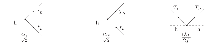
Figure 1: Feynman rules for couplings between the Higgs boson and the top quarks in the symmetric vacuum ($\langle h\rangle=0$). We have only shown those vertices relevant to the calculation of the one-loop quadratic divergences from the top sector. There are additional vertices, generated by terms of higher order in the expansion of $V$, involving three or more Higgs bosons.

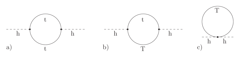
Figure 2: One-loop contributions to the Higgs boson (mass)² in the Little Higgs model.

The one-loop contribution to the Higgs boson (mass)² comes from the three diagrams in Fig. 2. The values of the diagrams are

a) $$= -6\lambda_{t}^{2}\int{d^{4}k\over(2\pi)^{4}}{1\over k^{2}},$$

b) $$= -6\lambda_{T}^{2}\int{d^{4}k\over(2\pi)^{4}}{1\over k^{2}-m_{T}^{2}},$$

c) $$= +6{\lambda_{T}\over f}\int{d^{4}k\over(2\pi)^{4}}{m_{T}\over k^{2}-m_{T}^{2}}.$$ (8)

The quadratic divergences neatly cancel. The top sector contribution to the Higgs (mass)² is then given by

$$\Delta m_{h}^{2}=-3{\lambda_{1}^{2}\lambda_{2}^{2}f^{2}\over 8\pi^{2}}\log{\Lambda^{2}\over m_{T}^{2}}=-3{\lambda_{t}^{2}m_{T}^{2}\over 8\pi^{2}}\log{\Lambda^{2}\over m_{T}^{2}}\ ,$$ (9)

where $\Lambda\sim 4\pi f$ is the strong interaction scale of the theory that gives rise to the Goldstone bosons. In Little Higgs models, $f$ is typically taken to be of order 1 TeV (corresponding to $\Lambda\sim 10$ TeV) to avoid fine tuning of the Higgs mass. As long as $m_{T}$ is parametrically lower than $\Lambda$, the negative contribution to $m_{h}^{2}$ in Equation (9) could be the dominant one and thus would provide the explanation for why electroweak symmetry is broken. There are incalculable (quadratically divergent) two-loop contributions to $m_{h}^{2}$, which are the same order in $\lambda_{1}\lambda_{2}$, but these are not logarithmically enhanced, and so are sub-dominant. The situation is that typically found in chiral perturbation theory.

The cancellation of quadratic divergences in Equation (8) depends on the relation of Equation (6), which can be rewritten as

$$\frac{m_{T}}{f}={\lambda_{t}^{2}+\lambda_{T}^{2}\over\lambda_{T}}\ .$$ (10)

The relation (10) is a very interesting one. All of the four parameters in this equation are in principle measurable. The top quark Yukawa coupling is known. The decay constant $f$ can be determined by measuring the properties of the heavy vector bosons in the Little Higgs theory [25]. The mass and couplings of the heavy top quark will be measured when this quark is observed, perhaps at the LHC. If the relation (10) is shown to be valid, that will be strong evidence for the picture of electroweak symmetry breaking given by the Little Higgs model.

3 How heavy is the heavy top quark?

If we are to study the heavy quark $T$, we should have some idea of what its mass is. The Little Higgs theory does not place a firm upper bound on the mass of the $T$. However, if the mass of the $T$ is greater than about 2 TeV, the cancellation shown in (8) requires some tuning to give an answer for $m_{h}$ below 220 GeV, the range for the Higgs boson mass preferred by precision electroweak measurements [30]. For this reason, the authors of [3] suggested that the mass of the $T$ should be less than 2 TeV.

On the other hand, the consistency of the Little Higgs model with precision electroweak data can place a lower limit on the mass of the $T$. The precision electroweak corrections from the model of [4] have been studied in some detail in [22] and [23]. These authors have found very strong bounds that imply $m_{T}>8$–10 TeV. The corrections from $T$ loops were computed in [22, 23], but these turned out to be relatively unimportant terms of order $\alpha m_{t}^{4}/m_{T}^{2}$. The large effects are the direct tree-level modifications of the precision electroweak predictions due to the new heavy vector bosons in the Little Higgs model. Consideration of their effects gives a lower bound on $f$. To find a limit on the mass of the $T$, we can use such a bound in conjunction with the inequality

$$\frac{m_{T}}{f}\geq 2\lambda_{t}\approx 2,$$ (11)

which is obtained by minimizing (10) with respect to $\lambda_{T}$.

There is a specific reason that the model of [4] leads to a very strong bound on $f$. In this model, all quadratically divergent contributions to $m_{h}^{2}$ due to $W$ and $Z$ boson loops are canceled by contributions from heavy gauge bosons. To achieve this, the authors of [4] make use of a gauge group $SU(2)\times SU(2)\times U(1)\times U(1)$. This leads to a multiplet of heavy $SU(2)$ gauge bosons and a heavy $U(1)$ gauge boson. The heavy $U(1)$ boson is actually not very heavy,

$$m\sim\frac{2}{\sqrt{5}}{g^{\prime}f}\ \approx 0.3\,f,$$ (12)

and this leads to large electroweak corrections, and also to problems with the direct observational bounds on $Z^{\prime}$ bosons from the Tevatron [22, 23].

3.1 An $SU(2)\times SU(2)\times U(1)$ model

There are various ways to ameliorate this problem [24], but the most direct is to gauge a smaller group. It has been suggested [31] that one might gauge only $SU(2)\times SU(2)\times U(1)$, canceling the quadratic divergences proportional to $g^{2}/4\pi$ but allowing quadratically divergent terms proportional to $g^{\prime 2}/4\pi$. Since $g^{\prime}$ is small, the latter are not unreasonably large if the cutoff or strong interaction scale $\Lambda$ of the Little Higgs model is about 10 TeV. In the remainder of this section, we will adopt this approach to find a more conservative lower bound on $f$ and on the $T$ quark mass.

The success of this approach depends on the exact choice of the symmetry-breaking pattern that produces the pseudo-Goldstone bosons of the Little Higgs models. Given the importance of the global $SU(3)$ symmetry for the top couplings, one might first study a model in which a global $SU(3)\times SU(3)$ symmetry is spontaneously broken to $SU(3)$. The multiplet of Goldstone bosons fill an adjoint representation of $SU(3)$. The Higgs field can be identified as an $SU(2)$ doublet within this structure,

$$2i\pi^{a}t^{a}=\frac{1}{\sqrt{2}}\pmatrix{0&0&h+i\pi^{3}\cr 0&0&-\sqrt{2}\pi^{-}\cr-(h-i\pi^{3})&\sqrt{2}\pi^{+}&0\cr}\ .$$ (13)

Exponentiating and taking the vacuum expectation value $\langle h\rangle=v=246$ GeV, we find the $SU(3)$ nonlinear sigma model field

$$V=e^{2i\pi^{a}t^{a}/f}=\pmatrix{\cos\frac{v}{\sqrt{2}f}&0&\sin\frac{v}{\sqrt{2}{f}}\cr 0&1&0\cr-\sin\frac{v}{\sqrt{2}{f}}&0&\cos\frac{v}{\sqrt{2}f}\cr},$$ (14)

The kinetic Lagrangian for this field is

$$\mathcal{L}={f^{2}\over 2}{\mbox{\rm tr}}\left[D_{\mu}V^{\dagger}D^{\mu}V\right]$$ (15)

with

$$D_{\mu}V=\partial_{\mu}V-ig_{L}A_{L\mu}^{a}T^{a}V+ig_{R}A_{R\mu}^{a}VT^{a}-ig^{\prime}B_{\mu}[Q,V].$$ (16)

Here, $T^{a}=\,$diag$\,(\tau^{a},0)$, where $\tau^{a}$ is an $SU(2)$ generator, and $Q$ is a matrix of $U(1)$ charges with $(-\frac{1}{2},\frac{1}{2},0)$ on the diagonal. Using these formulae, it is straightforward to work out the vector boson masses. To leading order in $v/f$, the heavy triplet of $W$’s have masses given by:

$$m_{W_{H}}^{2}=\frac{g_{L}^{2}+g_{R}^{2}}{2}f^{2}.$$ (17)

The masses of the usual $W$ and $Z$ turn out to be related by

$$m_{W}^{2}/m_{Z}^{2}=\cos^{2}\theta\left(1+{1\over 8}{v^{2}\over f^{2}}\right)\ ,$$ (18)

where $\cos^{2}\theta$ is the weak mixing angle defined in terms of the underlying gauge coupling constants. This gives an unacceptable violation of the known $W$/$Z$ mass relation if $f<3$ TeV. The problem stems from the fact that this model does not respect custodial $SU(2)$ at the level of $v^{2}/f^{2}$ corrections, as was pointed out already in the original papers of Georgi and Kaplan on pseudo-Goldstone models for the Higgs boson [32].

The symmetry breaking pattern $SU(5)/SO(5)$, which is the basis of [4], is much more promising from this point of view. In the old approach of Kaplan and Georgi, this model preserves custodial $SU(2)$. When we gauge $SU(2)\times SU(2)\times U(1)$ as in the Little Higgs models, custodial $SU(2)$ is explicitly broken, but it is possible to check that the custodial $SU(2)$-violating corrections to the vector boson mass relation (18) appear for the first time in order $v^{6}/f^{6}$. With this problem and that of the (too–light) heavy $U(1)$ boson removed, there is no further reason for a major difficulty with the precision electroweak data.

In the remainder of this section, we give some details of a more thorough analysis of this question. To begin, the Higgs doublet must be fit into the multiplet of Goldstone bosons of $SU(5)$ spontaneously broken to $SO(5)$. To do this, we write

$$2i\pi^{a}t^{a}={1\over\sqrt{2}}\pmatrix{0&0&(h+i\pi^{3})&0&0\cr 0&0&\sqrt{2}\pi^{-}&0&0\cr-(h-i\pi^{3})&-\sqrt{2}\pi^{+}&0&-(h+i\pi^{3})&-\sqrt{2}\pi^{-}\cr 0&0&(h-i\pi^{3})&0&0\cr 0&0&\sqrt{2}\pi^{+}&0&0\cr}\ ,$$ (19)

where we only show the degrees of freedom corresponding to the Higgs doublet.

It is convenient to take the vacuum configuration to be

$$V_{0}=\pmatrix{0&0&0&1&0\cr 0&0&0&0&1\cr 0&0&1&0&0\cr 1&0&0&0&0\cr 0&1&0&0&0\cr}\ .$$ (20)

Then, exponentiating the action of $\pi^{a}t^{a}$, we find the $SU(5)$ nonlinear sigma model field

$$V=e^{2i\pi^{a}t^{a}/f}V_{0}=\pmatrix{-\frac{1}{2}(1-c)&0&{s/\sqrt{2}}&\frac{1}{2}(1+c)&0\cr 0&0&0&0&1\cr-{s/\sqrt{2}}&0&c&-{s/\sqrt{2}}&0\cr\frac{1}{2}(1+c)&0&{s/\sqrt{2}}&-\frac{1}{2}(1-c)&0\cr 0&1&0&0&0\cr}\ ,$$ (21)

with

$$c=\cos{v\over f}\ ,\qquad s=\sin{v\over f}\ .$$ (22)

We now gauge the $SU(2)$ acting on the first two rows and columns of $V$ with gauge coupling $g_{L}$, the $SU(2)$ acting on the last two rows and columns of $V$ with gauge coupling $g_{R}$, and the unbroken $U(1)$ with coupling $g^{\prime}$. The normalization of the gauged $U(1)$ generator is chosen to ensure the correct value of the Higgs boson hypercharge. The kinetic Lagrangian for the $V$ field is

$$\mathcal{L}={f^{2}\over 4}{\mbox{\rm tr}}\left[D_{\mu}V^{\dagger}D^{\mu}V\right]\ .$$ (23)

Here the covariant derivative of the $V$ field is given by

$$D_{\mu}V=\partial_{\mu}V - i\sum_{j=L,R}g_{j}A^{a}_{j}(Q^{a}_{j}V+VQ^{aT}_{j})-ig^{\prime}B_{\mu}(YV+VY),$$ (24)

where $W^{a}_{j}$ ($a=1\ldots 3$) and $B$ are the $SU(2)$ and $U(1)$ gauge fields, respectively, and $g_{j}$ and $g^{\prime}$ are the corresponding gauge couplings. The generators are given by $Y=$ diag $(-1/2,-1/2,0,1/2,1/2)$ and

$$Q_{L}^{a}=\left(\begin{array}[]{ccc}\tau^{a}&&\\ &&\\ &&\end{array}\right),~{}~{}~{}~{}Q_{R}^{a}=\left(\begin{array}[]{ccc}&&\\ &&\\ &&-\tau^{a*}\end{array}\right).$$ (25)

We will assume that the left-handed fermions of the Standard Model transform as doublets under $SU(2)_{L}$ and singlets under $SU(2)_{R}$.

3.2 Vector boson mass matrices

From this starting point, it is not difficult to work out the masses and couplings of the vector bosons in this theory and compute their effect on the precision electroweak observables. In the basis $(A_{L}^{+},A_{R}^{+})$, the mass matrix of charged vector bosons is

$$m_{+}^{2}={f^{2}\over 2}\pmatrix{g_{L}^{2}&-\frac{1}{2}g_{L}g_{R}(1+c)\cr-\frac{1}{2}g_{L}g_{R}(1+c)&g_{R}^{2}\cr}.$$ (26)

The mass of the heavy $W$ gauge bosons to leading order is again given by Equation (17). Finding the masses of the usual $W$ and $Z$ to the precision that is necessary to compare with electroweak precision measurements requires a bit more work. Let

$$g^{2}={g_{L}^{2}g_{R}^{2}\over g_{L}^{2}+g_{R}^{2}}\ .$$ (27)

We can define a mixing angle $\psi$ by

$$g_{L}={g\over c_{\psi}}\ ,\qquad g_{R}={g\over s_{\psi}},$$ (28)

where $s_{\psi}\equiv\sin\psi$, $c_{\psi}\equiv\cos\psi$. In the basis

$$A_{(-)}=s_{\psi}A_{L}-c_{\psi}A_{R}\ ,\qquad A_{(+)}=c_{\psi}A_{L}+s_{\psi}A_{R}$$ (29)

the matrix $m_{+}^{2}$ is approximately diagonal. A further rotation of order $v^{2}/f^{2}$ is necessary to complete the diagonalization. The mass eigenstates are given by

$$W^{+}=s_{\beta}A_{(-)}^{+}+c_{\beta}A_{(+)}^{+}\ ,\qquad W_{H}^{+}=c_{\beta}A_{(-)}^{+}-s_{\beta}A_{(+)}^{+}\ ,$$ (30)

where

$$s_{\beta}\approx{v^{2}\over 4f^{2}}\,c_{\psi}s_{\psi}(c_{\psi}^{2}-s_{\psi}^{2}),\qquad c_{\beta}\approx 1.$$ (31)

Here and below, we neglect the terms of order $v^{4}/f^{4}$ and higher. The $W_{H}$ boson receives a mass of order $f\sim$ TeV, while the $W$ boson remains light. Its mass is given by

$$m_{W}^{2}={g^{2}v^{2}\over 4}\left[1-{v^{2}\over f^{2}}\left({1\over 12}+{1\over 8}(c_{\psi}^{2}-s_{\psi}^{2})^{2}\right)+\ldots\right].$$ (32)

The effective value of $G_{F}$, including the effect of the exchange of both vector bosons at $Q^{2}=0$, is

$${G_{F}\over\sqrt{2}} = {1\over 8}\pmatrix{g_{L}&0\cr}m_{+}^{-2}\pmatrix{g_{L}\cr 0\cr}$$ (33)

$$= {1\over 2v^{2}}\left[1+{5\over 24}{v^{2}\over f^{2}}\right]\ .$$

Similarly, the mass matrix of neutral vector bosons in the basis $(A_{L}^{3},A_{R}^{3},B)$ is given by

$$m_{0}^{2}={f^{2}\over 2}\pmatrix{g_{L}^{2}(1+\zeta)&-g_{L}g_{R}(\frac{1}{2}(1+c)+\zeta)&-\frac{1}{2}g_{L}g^{\prime}(1-c)\cr-g_{L}g_{R}(\frac{1}{2}(1+c)+\zeta)&g_{R}^{2}(1+\zeta)&-\frac{1}{2}g_{R}g^{\prime}(1-c)\cr-\frac{1}{2}g_{L}g^{\prime}(1-c)&-\frac{1}{2}g_{R}g^{\prime}(1-c)&g^{\prime 2}(1-c)\cr}\ ,$$ (34)

where $\zeta=(1-c)^{2}/8$. Comparing to (26), we see that the terms proportional to $\zeta$ in the matrix elements violate custodial $SU(2)$; however, these terms only contribute to $m_{W}/m_{Z}$ in order $v^{6}/f^{6}$. Let $\theta_{u}$ denote the “underlying” value of the weak mixing angle, defined by

$$g={e\over s_{u}}\ ,\qquad g^{\prime}={e\over c_{u}}\ ,\qquad$$ (35)

where $s_{u}\equiv\sin\theta_{u}$, $c_{u}\equiv\cos\theta_{u}$, and $e=gg^{\prime}/\sqrt{g^{2}+g^{\prime 2}}$. We can now proceed to the new basis:

$$A_{(-)}^{3},\qquad Z_{(0)}=c_{u}A^{3}_{(+)}-s_{u}B,\qquad A=s_{u}A^{3}_{(+)}+c_{u}B,$$ (36)

where $A_{(+)}$ and $A_{(-)}$ are defined in Equation (29). The state $A$ is an exact eigenvector of $m_{0}^{2}$ with a vanishing eigenvalue; we identify this state with the physical photon. The other two states in Equation (36) are not exact eigenvectors. As in the charged sector, a further rotation of order $v^{2}/f^{2}$ is needed to complete the diagonalization:

$$Z=s_{Z}A^{3}_{(-)}+c_{Z}Z_{(0)}\ ,\qquad Z_{H}=c_{Z}A^{3}_{(-)}-s_{Z}Z_{(0)}\ ,$$ (37)

where

$$s_{Z}\approx{v^{2}\over 4f^{2}}{c_{\psi}s_{\psi}\over c_{u}}(c_{\psi}^{2}-s_{\psi}^{2}),\qquad c_{Z}\approx 1.$$ (38)

The mass of the light $Z$ boson is given by

$$m_{Z}^{2}={g^{2}v^{2}\over 4c_{u}^{2}}\left[1-{v^{2}\over f^{2}}\left({1\over 12}+{1\over 8}(c_{\psi}^{2}-s_{\psi}^{2})^{2}\right)+\ldots\right],$$ (39)

while the $Z_{H}$ state obtains a mass of order $f\sim$ TeV.

3.3 Precision electroweak observables

From these formulae, we can work out the predictions for corrections to precision electroweak observables due to heavy gauge bosons. The reference value $\theta_{0}$ of the weak mixing angle is given by

$$\sin^{2}2\theta_{0}={4\pi\alpha\over\sqrt{2}G_{F}m_{Z}^{2}}.$$ (40)

From the formulae in Equations (33), (39) and (40), we can compute the shift between the underlying $s_{u}^{2}$ of Equation (35) and the reference value of $\sin^{2}\theta_{0}$, defined above:

$$s_{u}^{2}=s_{0}^{2}+\Delta s^{2}\ ,$$ (41)

with

$$\Delta s^{2}=\frac{1}{2}{v^{2}\over f^{2}}c^{2}_{\psi}s^{2}_{\psi}{c_{0}^{2}s_{0}^{2}\over c_{0}^{2}-s_{0}^{2}}.$$ (42)

Here, we have defined $s_{0}^{2}\equiv\sin^{2}\theta_{0},c_{0}^{2}=1-s_{0}^{2}$.

Using this formula and the expression for $s_{\beta}$ in Equation (31) to compute the coupling of leptons to the $Z^{0}$, we can compute the shifts of precision electroweak observables from their Standard Model tree-level values. For the three best-measured observables—$m_{W}$, the on-shell mass of the $W$, $s_{*}^{2}$, the effective value of the weak mixing angle in $Z^{0}$ decay asymmetries, and $\Gamma_{\ell}$, the leptonic width of the $Z^{0}$, we find

$$\Delta m_{W} \equiv m_{W}-m_{Z}c_{0}=-\frac{1}{2}{m_{W}\over c_{0}^{2}}\Delta s^{2},$$

$$\Delta s_{*}^{2} \equiv s_{*}^{2}-s_{0}^{2}=\Delta s^{2}-{1\over 4}{v^{2}\over f^{2}}s_{0}^{2}s_{\psi}^{2}(c_{\psi}^{2}-s_{\psi}^{2}),$$

$$\Delta\Gamma_{\ell} \equiv \Gamma_{\ell}-\Gamma_{\ell 0}=-\Gamma_{\ell 0}\left[\frac{1}{2}{v^{2}\over f^{2}}s^{4}_{\psi}+{4(1-4s_{0}^{2})\over 1-4s_{0}^{2}+8s_{0}^{4}}\Delta s^{2}\right],$$ (43)

where

$$\Gamma_{\ell 0}={4\pi e^{2}m_{Z}\over 6s_{0}^{2}c_{0}^{2}}\left((\frac{1}{2}-s_{0}^{2})^{2}+s_{0}^{4}\right)$$ (44)

is the Standard Model tree-level value of the leptonic width of the $Z$.

We can interpret these shifts as a contribution to the $S$ and $T$ parameters [33]. Formally, effects on the precision electroweak parameters due to extra $Z$ and $W$ bosons are not oblique and cannot be completely absorbed into $S$ and $T$. However, it was observed in [34] that a fit to the electroweak data with the shifts from a $Z^{\prime}$ and compensatory values of $S$ and $T$ was comparable in quality to a fit to the Standard Model; the opposite of the values of $S$ and $T$ needed to compensate the effect of the $Z^{\prime}$ could then be viewed as the $(S,T)$ excursion due to the $Z^{\prime}$.

Applying this method to the $SU(5)/SO(5)$ Little Higgs model with $SU(2)\times SU(2)\times U(1)$ gauged, using the observables in (43), we find that the effect of the model on the precision electroweak data is represented by the $(S,T)$ excursions shown in Fig. 3 and Fig. 4. In producing the fit, we use [35]

$$m_{W} = 80.425\pm 0.034\mbox{ GeV},$$ (45)

$$s_{\ast}^{2} = 0.23150\pm.00016,$$ (46)

$$\Gamma_{\ell} = 83.984\pm 0.086\mbox{ MeV}.$$ (47)

We allow the values of the top quark mass and the electromagnetic coupling to vary within their current errors: $m_{t}=174.3\pm 5.1$ GeV, $\alpha^{-1}(m_{Z})=128.936\pm 0.021$ [35]. All effects shown in (43) become very small as $s_{\psi}\to 0$, allowing lower values of $f$ to be consistent with the electroweak constraints. The constraint cannot be eliminated completely, since according to Equation (28) the gauge coupling $g_{R}$ becomes strong as $s_{\psi}\to 0$ and the perturbative analysis performed here is no longer applicable. Still, the bounds on $f$ are not very strong: for example, for $s_{\psi}=0.2$ (corresponding to $g_{R}^{2}/4\pi\approx 0.4$, which is probably not yet strong coupling), we find that $f$ can be lower than 1 TeV within the 68% confidence region of the electroweak fit.

Our analysis includes the shifts of the electroweak precision observable due to heavy gauge bosons, but does not include possible corrections from a vacuum expectation value (vev) for the $SU(2)$ triplet pseudo-Goldstone boson present in this model. These corrections can play an important role in constraining the model for small values of $s_{\psi}$ [24]. The value of the triplet vev is not calculable from the low-energy effective Little Higgs theory, and including it in the analysis corresponds to adding an extra free parameter to the model. The bounds in Fig. 3 and Fig. 4 are valid in the regions of the parameter space where the triplet vev is small, but may underestimate the constraints in other regions. A more detailed analysis that includes the contribution of the triplet vev can be found in Ref. [24].

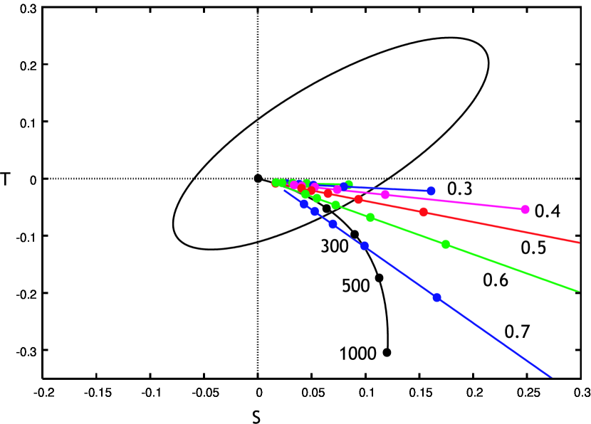
Figure 3: Excursions in the $S-T$ plane resulting from the $SU(5)/SO(5)$ Little Higgs model with a single gauged $U(1)$. The different lines represent different values of $\sin\psi$={0.1, 0.2, 0.3, …0.7 }, while the points on the lines represent different values of $f$. The rightmost point (not visible for $\sin\psi=\{0.5,0.6,0.7\}$) is for 1 TeV, and additional points are separated by 500 GeV, increasing in $f$. The ellipse represents the experimentally allowed region at the 68% confidence level for two degrees of freedom. Also shown is the dark black curve showing the $S$ and $T$ contributions of a Standard Model Higgs boson for various masses. We provide an enlargement of this figure in Fig. 4. Note that the lines for $\sin\psi$={0.1, 0.2} are somewhat obscured here, but can be seen clearly in Fig. 4.

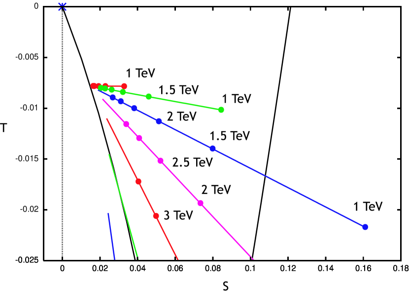
Figure 4: This figure is an enlargement of the central portion of Fig. 3, focusing on points compatible with the electroweak precision measurements. The uppermost line is for $\sin\psi$=0.1. Each line represents an increment of 0.1 in $\sin\psi$. The Higgs mass is set to $115$ GeV in the Little Higgs model, while $S=T=0$ is defined for $m_{h}$=100 GeV.

Since all three of the measurements in (43) are made at the $Z$ and $W$ poles, one should ask whether low-$Q^{2}$ observables can put further constraints on the parameters of the Little Higgs theory. To analyze this, we have computed the effective low-energy neutral current Lagrangian, in the form

$$\mathcal{L}_{\rm\tt NC}={G_{F}\over\sqrt{2}}\rho\left[(J^{3}_{\mu}-s_{\nu}^{2}J^{Q}_{\mu})^{2}+\eta J^{Q}_{\mu}J^{Q\mu}\right]\ .$$ (48)

In the Standard Model at tree level, $\rho=1$, $s_{\nu}^{2}=s_{0}^{2}$, $\eta=0$. In the $SU(5)/SO(5)$ model, we find $\rho=1$, up to corrections of order $v^{6}/f^{6}$, and

$$s_{\nu}^{2}-s_{0}^{2} = s_{0}^{2}\cdot{1\over 4}{v^{2}\over f^{2}}s_{\psi}^{2}\left[{2c_{0}^{2}c_{\psi}^{2}\over c_{0}^{2}-s_{0}^{2}}-1\right],$$

$$\eta = s_{0}^{4}\cdot\frac{1}{2}{v^{2}\over f^{2}}s^{4}_{\psi}\ .$$ (49)

For points in the region allowed by the $(S,T)$ analysis, the shifts in $s_{\nu}^{2}$ are very small. For example, for $s_{\psi}^{2}=0.2$ and $f=1$ TeV, $s_{\nu}^{2}-s_{0}^{2}\approx 10^{-4}$. The parameter $Q_{W}$ of atomic parity violation [36] and the observables $R^{\nu}$, $R^{\overline{\nu}}$ measured by the NuTeV experiment [37] depend on $s_{\nu}^{2}$ but do not involve $\eta$. In all cases, the effects on these parameters are corrections of relative size less than $10^{-3}$, well within the current experimental errors.

Through (11), the lower bound on $f$ from the precision electroweak observables places a strong lower bound of about 2 TeV on the mass of the $T$. However, this still leaves a range in which the $T$ can be discovered at the LHC. It is worth emphasizing that a $T$ mass much higher than 2 TeV would imply a large amount of fine tuning in the Higgs potential. Therefore, naturalness considerations together with precision electroweak constraints indicate that if the Little Higgs model is correct, the heavy top should be in the 2 TeV range. In this case, it is possible that the physics of electroweak symmetry breaking in the Little Higgs model can be tested at LHC. We now turn to the analysis of those experimental tests. For our analyses in the next section, we assume a heavy top mass of 2.5 TeV and $f$=1.2 TeV, which is clearly allowed by the precision electroweak observables.

4 Testing the Model at the LHC

To test the relation (10), it is necessary to measure three quantities, the parameter $f$, the mass $m_{T}$, and the coupling constant $\lambda_{T}$. The measurement of the mass and production cross section of the heavy $SU(2)$ gauge bosons $W_{H},Z_{H}$ at the LHC can be used to determine $f$ [25]. We will review the strategy for this measurement below, concentrating on the low values of the mixing angle, $\psi$, preferred by precision electroweak constraints. The measurement of the heavy top mass $m_{T}$ is rather straightforward; on the other hand, it is much less clear how $\lambda_{T}$ can be determined. In this section, we will discuss two methods for measuring $\lambda_{T}$. These involve the decay width and the production cross section for $T$ quarks at the LHC.

4.1 Measuring the parameter $f$

In the $SU(5)/SO(5)$ Little Higgs model described in section 3, all the couplings involving the heavy gauge bosons $W_{H}^{\pm}$ and $Z_{H}$ depend on just two unknown parameters, the scale $f$ and the mixing angle $\psi$, defined in Equation (28). Thus, a small number of measurements in this sector is sufficient to determine both parameters. Let us concentrate on the measurements involving the neutral gauge boson $Z_{H}$. To leading order in $v/f$, the $Z_{H}$ mass is given by

$$M_{Z_{H}}=\sqrt{\frac{g_{L}^{2}+g_{R}^{2}}{2}}f=\frac{\sqrt{2}g}{\sin 2\psi}\,f.$$ (50)

The production cross section and decay branching ratios of $Z_{H}$ bosons have been obtained in [25]. For fixed $M_{Z_{H}}$, the production cross section is proportional to $\tan^{2}\psi$. The decay rate is given by

$$\Gamma=\frac{g^{2}}{96\pi}\,(\cot^{2}2\psi+24\tan^{2}\psi)\,M_{Z_{H}}\,,$$ (51)

with the branching ratios

$${\rm Br}(\ell\overline{\ell}) = \frac{1}{3}\,{\rm Br}(q\overline{q})=\frac{\tan^{2}\psi}{\cot^{2}2\psi+24\tan^{2}\psi};$$

$${\rm Br}(W^{+}W^{-}) = {\rm Br}(Zh)=\frac{1}{2}\,\frac{\cot^{2}2\psi}{\cot^{2}2\psi+24\tan^{2}\psi}.$$ (52)

From these formulae, it is clear that combining, for example, the measurement of the $Z_{H}$ mass and the number of events in the $\ell^{+}\ell^{-}$ ($\ell=e$ or $\mu$) channels is sufficient to determine both $f$ and $\psi$.

In the parameter region preferred by electroweak precision constraints, the dominant decay modes are $Z_{H}\to W^{+}W^{-}$ and $Z_{H}\to Zh$. For example, for $s_{\psi}=0.2$, the combined branching ratio of these two modes is about 85%, with the remaining decays to fermion pairs. The branching ratio to leptons ($e$’s and $\mu$’s) is only about 1%. Nevertheless, for an $f=1.2$ TeV the production cross section for the $Z_{H}$ is roughly 12 fb, corresponding to 3600 events in a 300 fb^-1 data sample. Therefore, in the lepton channels we still expect roughly 40 events, with virtually no background. Studying these events should be sufficient to determine $f$ and $\psi$. Of course, the events in the other decay channels, along with the decays of $W_{H}^{\pm}$, will only help to improve the precision of the determination of $f$.

4.2 Measuring $\lambda_{T}$

4.2.1 Decays of the $T$ quark

Since $T$ has a vertex for $T\to th$, as shown in Fig. 1, the heavy $T$ quark will decay to $th$, and the corresponding decay width is proportional to $\lambda_{T}^{2}$. But $T$ also has other decay modes. This is made clear by looking at the ‘gaugeless limit’ [39] $g\to 0$, in which the weak bosons become massless and the Goldstone bosons of $SU(2)\times U(1)$ breaking become physical. In this limit, the structure of (3) ensures that $T$ decays symmetrically to the four members of the Higgs $SU(2)$ doublet: $\Gamma(T\to th)=\Gamma(T\to t\pi^{3})=\frac{1}{2}\Gamma(T\to b\pi^{+})$. In the real situation, $\pi^{+}$ and $\pi^{3}$ are replaced by the longitudinal polarization states of the $W^{+}$ and $Z^{0}$ vector bosons:

$$\Gamma(T\to th)\approx\Gamma(T\to tZ^{0})\approx\frac{1}{2}\Gamma(T\to bW^{+})\ .$$ (53)

All three decay modes provide characteristic signatures for the discovery of the $T$ at the LHC.

We will now obtain more exact relations for the decay branching ratios of the $T$ and, at the same time, see how the approximate equalities (53) work when the Standard Model gauge couplings are turned back on. To do this, we must diagonalize the top quark mass matrix more carefully, picking up terms that we dropped in the discussion leading to (7). In principle, we should also modify (3) to take into account the constraints from using an $SU(5)/SO(5)$ nonlinear sigma model. However, this model belongs to the general class of models for which the formulae of Section 2 are precisely valid. To see this explicitly, the invariant Lagrangian can be written in terms of $SU(5)/SO(5)$ Goldstone bosons as [4]

$$\mathcal{L}=-{\lambda_{1}\over 2}f\,\overline{u}_{R}\epsilon_{ijk}\epsilon_{mn}V_{im}V_{jn}\chi_{Lk}-\lambda_{2}f\,\overline{U}_{R}U_{L}+{\rm h.c.}\ ,$$ (54)

where $V_{im}$ denotes the $3\times 2$ upper right hand block of $V$ in (21). The relevant Feynman rules for the top quarks are just those shown in Fig. 1. According to Equation (26), $f$ is again given in terms of the heavy boson masses by Equation (17), and is fixed to be roughly greater than 1 TeV by the arguments of the previous section.

Now let us consider the heavy quark mass diagonalization more carefully. In particular, if we include the $SU(2)\times U(1)$-breaking vacuum expectation value $v$, the top quark mass matrix becomes

$$\pmatrix{\overline{u}_{R}&\overline{U}_{R}\cr}m_{U}\pmatrix{u_{L}\cr U_{L}\cr},\$$ (55)

with

$$m_{U}=f\pmatrix{\frac{\lambda_{1}s}{\sqrt{2}}&\frac{\lambda_{1}}{2}(1+c)\cr 0&\lambda_{2}\cr}\ .$$ (56)

Here, we have again used $s\equiv\sin\frac{v}{f}$ and $c\equiv\cos\frac{v}{f}$. Diagonalizing $m_{U}^{\dagger}m_{U}$, we find the mixing angle for the left-handed components of the top quarks,

$$\theta_{t}=\frac{1}{2}\tan^{-1}\frac{2\sqrt{2}\lambda_{1}^{2}s(1+c)}{4\lambda_{2}^{2}+(1+c)^{2}\lambda_{1}^{2}-2\lambda_{1}^{2}s^{2}}\approx{1\over\sqrt{2}}{\lambda_{1}^{2}\over\lambda_{1}^{2}+\lambda_{2}^{2}}{v\over f}\ \approx{\lambda_{T}v\over\sqrt{2}m_{T}}$$ (57)

Let $\cos\theta_{t}=c_{t}$, $\sin\theta_{t}=s_{t}$; then the mass eigenstates are given by

$$T_{L} = c_{t}U_{L}+s_{t}u_{L},$$

$$t_{L} = -s_{t}U_{L}+c_{t}u_{L}\ .$$ (58)

There is also a mixing angle for the right-handed quarks, $\theta_{tr}$, given by

$$T_{R} = c_{tr}U_{R}+s_{tr}u_{R},$$

$$t_{R} = -s_{tr}U_{R}+c_{tr}u_{R}\ .$$ (59)

Note that this angle is non-zero even in the absence of electroweak symmetry breaking, see Equation (5).

From the mixing, the top quark mass receives a small correction,

$$m_{t}={\lambda_{t}v\over\sqrt{2}}\left(1-\left(\frac{1}{6}-\frac{\lambda_{1}^{2}\lambda_{2}^{2}}{4(\lambda_{1}^{2}+\lambda_{2}^{2})^{2}}\right){v^{2}\over f^{2}}+\cdots\right)\ .$$ (60)

For $f=1.2$ TeV, this is a 0.3% correction to the Standard Model tree level relation. In the following, we will quote ‘exact’ tree-level relations in terms of $m_{t}$, $m_{T}$, $\lambda_{T}$, and $\theta_{t}$ and their leading-order terms in an expansion in $v/f$. Typically, these expressions will agree to within a few percent.

The admixture of $u_{L}$ in the $T$ allows this quark to decay by the Standard Model weak currents. The amplitudes for the decay modes to $W^{+}$ and $Z^{0}$ are then proportional to $\sin\theta_{t}$. However, the contraction of the longitudinal polarization vector of a massive vector boson with the spontaneously broken weak current gives an enhancement by a factor $m_{T}/m_{W}$, so that the full coupling is of the order of

$${g\over\sqrt{2}}\left({m_{T}\over m_{W}}\right)\theta_{t}=\sqrt{2}{m_{T}\over v}\theta_{t}=\lambda_{T}\ .$$ (61)

This allows the three branching fractions of the $T$ to be of the same order of magnitude. A similar effect is well known in the decays of the singlet $D$ quark in $E_{6}$ models [40].

Working more explicitly, we find for the three dominant partial widths of the $T$ quark:

$$\Gamma(T\to th) = {\lambda_{1}^{2}\,m_{T}\over 64\pi}f(x_{t},x_{h})[(1+x_{t}^{2}-x_{h}^{2})(C_{L}^{2}+C_{R}^{2})+4C_{L}C_{R}x_{t}]$$

$$\approx {m_{T}\lambda_{T}^{2}\over 64\pi},$$

$$\Gamma(T\to tZ^{0}) = {e^{2}\sin^{2}2\theta_{t}m_{T}^{3}c_{Z}^{2}\over 512\pi M_{Z}^{2}s_{u}^{2}c_{u}^{2}}(1+\tan_{\psi}c_{u}\tan_{Z})^{2}\,f(x_{Z},x_{b})\,g(x_{b},x_{Z})$$

$$\approx {m_{T}\lambda_{T}^{2}\over 64\pi},$$

$$\Gamma(T\to bW^{+}) = {g^{2}\sin^{2}\theta_{t}m_{T}^{3}c_{\beta}^{2}\over 64\pi M_{W}^{2}}(1+\tan_{\psi}\tan_{\beta})^{2}\,f(x_{W},x_{b})\,g(x_{b},x_{W})$$ (62)

$$\approx {m_{T}\lambda_{T}^{2}\over 32\pi}.$$

Note that $s_{Z}$, defined in Equation (37), and $s_{\beta}$, defined in Equation (30), are both of order $v^{2}/f^{2}$. We have defined $x_{i}\equiv m_{i}/m_{T}$, the kinematic functions

$$f(x_{i},x_{j}) = \sqrt{(1-(x_{i}+x_{j})^{2})(1-(x_{i}-x_{j})^{2})},$$

$$g(x_{i},x_{j}) = (1-x_{i}^{2})+x_{j}^{2}(1+x_{i}^{2})-2x_{j}^{4},$$ (63)

and introduced the couplings

$$C_{L}=c_{tr}(s_{t}\cos{\frac{v}{f}}-{c_{t}\over\sqrt{2}}\sin{\frac{v}{f}})\sim{\mathcal{O}}\left({v\over f}\right),$$

$$C_{R}=s_{tr}(c_{t}\cos{\frac{v}{f}}+{s_{t}\over\sqrt{2}}\sin{\frac{v}{f}})\sim{\mathcal{O}}\left(1\right).$$ (64)

To leading order in $v^{2}/f^{2}$, the total width of the $T$ is then

$$\Gamma_{T}={m_{T}\lambda_{T}^{2}\over 16\pi}.$$ (65)

The measurement of this total width is the first possible method for measuring $\lambda_{T}$. However, it is not so easy to measure the width of a strongly interacting particle produced at a hadron collider, because the fluctuations of QCD jets lead to an intrinsic smearing of the mass peak. For the ATLAS detector, the fractional uncertainty in the two-jet invariant mass at 2.5 TeV is expected to be about $\pm 5$% [41], which for a heavy top of $2.5$ TeV, corresponds to a minimal error of $\pm 125$ GeV in the width. On the other hand, for $m_{T}=2.5$ TeV and $\lambda_{T}\approx\lambda_{t}$, the formula (65) evaluates to only 50 GeV. With these estimates, $\Gamma_{T}$ will be only marginally visible, and then only if the jet mass resolution is very well understood theoretically. Therefore, it appears challenging to use this strategy to make the test of the Little Higgs model described here.

4.2.2 Production of the $T$ quark

Another possible strategy is to extract $\lambda_{T}$ from a measurement of the $T$ production cross section at the LHC. For $m_{T}$ above 2 TeV, energy is at a premium and the single-$T$ production reaction $pp\to T+X$ dominates over the pair-production of $T$’s via strong interactions, $pp\to T+\overline{T}$. At the parton level, the dominant mechanism of single-$T$ production is through the “$W-b$ fusion” reaction [26]

$$qb\to q^{\prime}T,$$ (66)

shown in Fig. 5. The cross section for this reaction is dominated by the exchange of a longitudinal $W$ boson, whose coupling to $T$ is proportional to $\lambda_{T}$ (see Equation (61)). Thus, a measurement of this cross section would determine the value of $\lambda_{T}$, providing a test of the crucial relation (10).

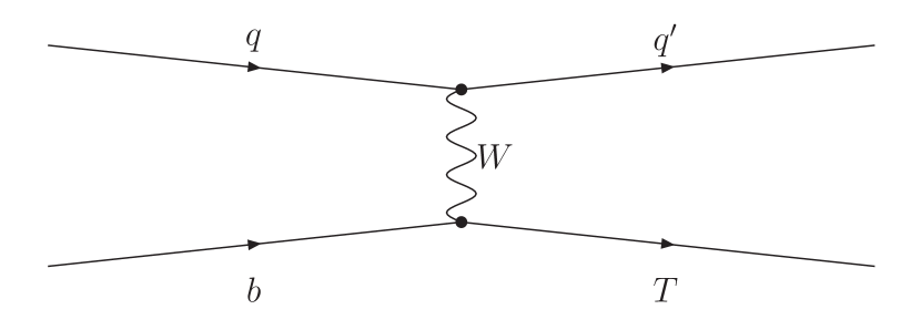
Figure 5: The dominant process for $T$ production at the LHC.

How well can this cross section be measured at the LHC? The answer obviously depends on the mass of the $T$ quark, as well as on the size of the coupling $\lambda_{T}$. In Figure 6, we plot the expected cross section as a function of $m_{T}$, for $\lambda_{T}=1/\sqrt{3},1$, and $\sqrt{3}$ using the CTEQ4l parton distribution functions. For $\lambda_{T}$ not too small, the number of events is large enough to keep the statistical uncertainty under control: for example, for $m_{T}=2.5$ TeV and $\lambda_{T}=1$, the evaluated production cross section corresponds to roughly 180 events for a 300 fb^-1 data sample. The reaction is characterized by a $T$ decay at low transverse momentum and in the central region, and all other jet activity very forward. All three of the decay modes discussed above should be identifiable. The final states $T\rightarrow th^{0}\rightarrow tb\overline{b}$ and $T\rightarrow bW^{+}\rightarrow bl^{+}\nu$ can be required with high efficiency and used to find a $T$ mass peak. In the latter case, one should replace the observed $l^{+}$ with a $W^{+}$ in the $l^{+}$ direction.

Also shown in the figure are two parabolas, which represent the predictions of the model for two representative values of $f$. Once the $f$ value is determined as described in Section 4.1, the electroweak symmetry breaking mechanism described here predicts that the values of $m_{T}$ and the production cross section lie on the corresponding parabola.

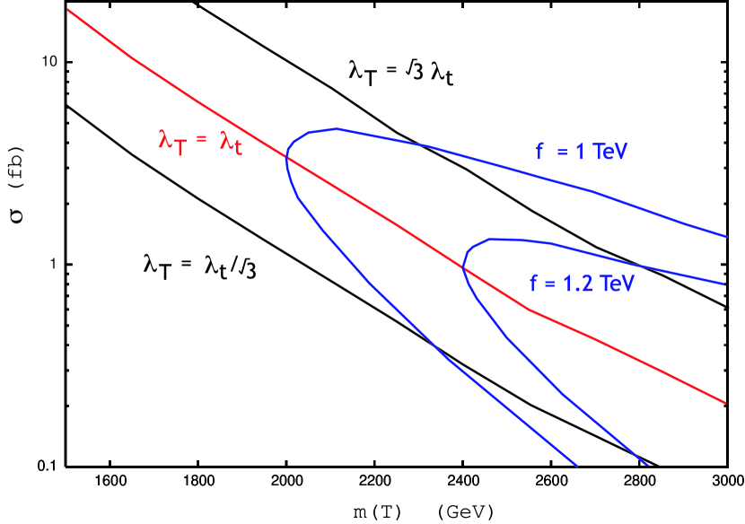
Figure 6: Parton level production cross section for the heavy top in the channel $bq\rightarrow Tq\prime$ at the 14 TeV Large Hadron Collider. The figure is made with the CTEQ4l parton distribution function. The different lines show the difference in the production cross section for various values of $\lambda_{T}$. The parabolas represent the predictions of the Little Higgs model for a constant $f$ as $\lambda_{T}$ is varied.

Converting a cross section measurement into a measurement of the coupling $\lambda_{T}$ requires knowledge of the parton distribution functions (pdfs) of the initial state particles. Since the typical energies involved are much larger than the $W$ boson mass, it is reasonable to use the effective-$W$ approximation, which treats the $W$ as a parton within the proton. In this approximation, the single-$T$ production is described as a $2\to 1$ process, $bW\to T$. The cross section is given by

$$\sigma(pp\to T+X)\,=\,\int_{0}^{1}\,dx_{b}\,f_{b}(x_{b},Q^{2})\,f_{w}(\frac{m_{T}^{2}}{x_{b}S},Q^{2})\,\hat{\sigma}(Wb\to T),$$ (67)

where $f_{b,w}$ are the pdfs of the $b$ quark and the $W$ boson, $\hat{\sigma}$ is the parton-level cross section, $S$ is the usual Mandelstam variable, and $Q$ is the renormalization scale, $Q^{2}\sim m_{T}^{2}$. The $b$ quark pdf is derived perturbatively from the gluon pdf [42, 43, 44]. The integral in (67) receives significant contributions from the region where $x\approx m_{T}/\sqrt{S}$. At the LHC, $\sqrt{S}=14$ TeV, and this region can extend to $x$ as high as $\sim 0.2$ for the values of the $T$ mass considered here. Currently, our knowledge of the $b$ pdf in the large-$x$ region is rather poor: the uncertainty on $f(x_{b})$ is about 20% for $x_{b}=0.1$ and even higher for higher $x_{b}$ [45]. Without reducing this uncertainty, even a very accurate measurement of the single-$T$ production cross section would not provide a precision test of the relation (10).

One possible way to reduce the uncertainty is to obtain an accurate measurement of the cross section of the Standard Model single top production at the Tevatron. While there are several contributions to this process, the cross section is dominated by the $Wb$ fusion process, $Wb\to t$, and it has been shown [46] that this contribution to the cross section can be isolated using kinematic cuts. A significant fraction of the events in this channel are initiated by $b$ quarks with $0.1\mathrel{\mathchoice{\lower 2.5pt\vbox{\halign{$\mathsurround 0pt\displaystyle\hfil#\hfil$\cr<\crcr\sim\crcr}}}{\lower 2.5pt\vbox{\halign{$\mathsurround 0pt\textstyle\hfil#\hfil$\cr<\crcr\sim\crcr}}}{\lower 2.5pt\vbox{\halign{$\mathsurround 0pt\scriptstyle\hfil#\hfil$\cr<\crcr\sim\crcr}}}{\lower 2.5pt\vbox{\halign{$\mathsurround 0pt\scriptscriptstyle\hfil#\hfil$\cr<\crcr\sim\crcr}}}}x_{b}\mathrel{\mathchoice{\lower 2.5pt\vbox{\halign{$\mathsurround 0pt\displaystyle\hfil#\hfil$\cr<\crcr\sim\crcr}}}{\lower 2.5pt\vbox{\halign{$\mathsurround 0pt\textstyle\hfil#\hfil$\cr<\crcr\sim\crcr}}}{\lower 2.5pt\vbox{\halign{$\mathsurround 0pt\scriptstyle\hfil#\hfil$\cr<\crcr\sim\crcr}}}{\lower 2.5pt\vbox{\halign{$\mathsurround 0pt\scriptscriptstyle\hfil#\hfil$\cr<\crcr\sim\crcr}}}}0.2$; the remaining events almost exclusively come from the region $x_{b}<0.1$, where the $b$ pdf is known much more accurately. Thus, assuming that the value of $V_{tb}$ and the $W$ boson pdf are known, a measurement of $\sigma(p\overline{p}\to t+X)$ with the relevant cuts can be interpreted as a measurement of $f_{b}(x_{b},Q^{2})$ at $x_{b}\sim 0.1-0.2$ and $Q^{2}\sim m_{t}^{2}$. This knowledge can then be used to reduce the uncertainty of the theoretical prediction for the $T$ quark production at the LHC. Since $b$ is a sea quark, the $b$ pdfs in the proton and anti-proton are virtually identical, and the fact that the Tevatron is a $p\overline{p}$ collider introduces no additional complications. Evolution of the $b$ pdf from $Q^{2}\sim m_{t}^{2}$ to $Q^{2}\sim m_{T}^{2}$ can be performed perturbatively. It is well known that $f_{b}(x,Q^{2})$ decreases with increasing $Q^{2}$ at large $x$ and increases with $Q^{2}$ at small $x$. Interestingly, the cross over point for $Q^{2}\sim$ (1 TeV)² falls in the range of $x$ most relevant for the present discussion, $x\approx 0.18$. For $0.14<x<0.2$, $f_{b}(x)$ varies by only a few percent going from $Q^{2}$=(175 GeV)² to $Q^{2}=$ (2 TeV)². Therefore, measurements of $f_{b}(x,Q^{2})$ at the Tevatron can be extrapolated to the LHC with controllable uncertainty. The statistical uncertainty in the measurement of $\sigma(p\overline{p}\to t+X)$ at the Tevatron is expected to be about 5% for 2 fb^-1 integrated luminosity [47]. While a more detailed investigation is in order, it seems plausible that this method could result in a measurement of $\lambda_{T}^{2}$ at the level of 10% or better.

5 Conclusions

The Little Higgs model provides a simple mechanism for electroweak symmetry breaking, relying on the top sector to trigger a negative (mass)² for the Higgs boson. This mechanism depends on a simple relation between the parameters of the model, summarized in Equation (10). In principle, all parameters in this equation are measurable, providing a strong test of the mechanism. The testability of this relation at the LHC depends on the heavy top quark partner, $T$, being sufficiently light (roughly 2 TeV), as is favored by naturalness arguments. We have shown that such a light $T$ can be consistent with current electroweak precision measurements.

The most challenging of the required measurements is the determination of $\lambda_{T}$, the coupling of the heavy top to the Higgs boson. We have outlined two strategies: measuring the width of the $T$ and measuring its production cross-section. The first strategy, limited by calorimeter resolution, is not very promising. The second strategy can be more successful if the pdfs of the $b$ quark can be determined more accurately at high $x$. This may indeed be possible using the measurement of single top production from the current run at the Tevatron.

More detailed Monte Carlo studies to determine the feasibility of the measurements outlined here would be worthwhile.

ACKNOWLEDGEMENTS

We are grateful to Nima Arkani-Hamed, Gustavo Burdman, Csaba Csaki, Patrick Meade, Frank Petriello, Tim Tait, and Jay Wacker for valuable advice. MEP thanks Kiwoon Choi and his students for valuable discussions that ignited his interest in the topics considered here. We thank Hitoshi Murayama for suggesting an improvement of our S,T fitting procedure. M. P. completed a part of this work at Lawrence Berkeley National Laboratory, where he was supported by the Director, Office of Science, Office of High Energy and Nuclear Physics, of the U. S. Department of Energy under Contract DE-AC03-76SF00098.

References

- [1] N. Arkani-Hamed, A. G. Cohen and H. Georgi, Phys. Lett. B 513, 232 (2001) [arXiv:hep-ph/0105239].
- [2] N. Arkani-Hamed, A. G. Cohen, T. Gregoire and J. G. Wacker, JHEP 0208, 020 (2002) [arXiv:hep-ph/0202089].
- [3] N. Arkani-Hamed, A. G. Cohen, E. Katz, A. E. Nelson, T. Gregoire and J. G. Wacker, JHEP 0208, 021 (2002) [arXiv:hep-ph/0206020].
- [4] N. Arkani-Hamed, A. G. Cohen, E. Katz and A. E. Nelson, JHEP 0207, 034 (2002) [arXiv:hep-ph/0206021].
- [5] M. Schmaltz, Nucl. Phys. Proc. Suppl. 117, 40 (2003) [arXiv:hep-ph/0210415].
- [6] J. G. Wacker, arXiv:hep-ph/0208235.
- [7] H. Georgi and A. Pais, Phys. Rev. D 12, 508 (1975).
- [8] D. B. Kaplan and H. Georgi, Phys. Lett. B 136, 183 (1984).
- [9] D. B. Kaplan, H. Georgi and S. Dimopoulos, Phys. Lett. B 136, 187 (1984).
- [10] K. Inoue, A. Kakuto, H. Komatsu and S. Takeshita, Prog. Theor. Phys. 68, 927 (1982) [Erratum-ibid. 70, 330 (1983)].
- [11] L. E. Ibanez, Nucl. Phys. B 218, 514 (1983); L. E. Ibanez and C. Lopez, Phys. Lett. B 126, 54 (1983).
- [12] J. R. Ellis, J. S. Hagelin, D. V. Nanopoulos and K. Tamvakis, Phys. Lett. B 125, 275 (1983).
- [13] L. Alvarez-Gaume, J. Polchinski and M. B. Wise, Nucl. Phys. B 221, 495 (1983).
- [14] C. T. Hill, Phys. Lett. B 266, 419 (1991), Phys. Lett. B 345, 483 (1995) [arXiv:hep-ph/9411426].
- [15] A. E. Nelson, arXiv:hep-ph/0304036.
- [16] I. Low, W. Skiba and D. Smith, Phys. Rev. D 66, 072001 (2002) [arXiv:hep-ph/0207243].
- [17] D. E. Kaplan and M. Schmaltz, arXiv:hep-ph/0302049.
- [18] S. Chang and J. G. Wacker, arXiv:hep-ph/0303001.
- [19] T. Gregoire, D. R. Smith and J. G. Wacker, arXiv:hep-ph/0305275.
- [20] W. Skiba and J. Terning, arXiv:hep-ph/0305302.
- [21] S. Chang, arXiv:hep-ph/0306034.
- [22] C. Csaki, J. Hubisz, G. D. Kribs, P. Meade and J. Terning, Phys. Rev. D 67, 115002 (2003) [arXiv:hep-ph/0211124].
- [23] J. L. Hewett, F. J. Petriello and T. G. Rizzo, arXiv:hep-ph/0211218.
- [24] C. Csaki, J. Hubisz, G. D. Kribs, P. Meade and J. Terning, Phys. Rev. D 68, 035009 (2003) [arXiv:hep-ph/0303236].
- [25] G. Burdman, M. Perelstein and A. Pierce, Phys. Rev. Lett. 90, 241802 (2003) [arXiv:hep-ph/0212228].
- [26] T. Han, H. E. Logan, B. McElrath and L. T. Wang, Phys. Rev. D 67, 095004 (2003) [arXiv:hep-ph/0301040].
- [27] T. Han, H. E. Logan, B. McElrath and L. T. Wang, Phys. Lett. B 563, 191 (2003) [arXiv:hep-ph/0302188].
- [28] B. A. Dobrescu and C. T. Hill, Phys. Rev. Lett. 81, 2634 (1998) [arXiv:hep-ph/9712319]; R. S. Chivukula, B. A. Dobrescu, H. Georgi and C. T. Hill, Phys. Rev. D 59, 075003 (1999) [arXiv:hep-ph/9809470].
- [29] A. Jarry, Ubu Roi, Paris: Mercure de France, 1896.
- [30] http://lepewwg.web.cern.ch/LEPEWWG/
- [31] N. Arkani-Hamed and J. Wacker, personal communication.
- [32] H. Georgi and D. B. Kaplan, Phys. Lett. B 145, 216 (1984).
- [33] M. E. Peskin and T. Takeuchi, Phys. Rev. Lett. 65, 964 (1990), Phys. Rev. D 46, 381 (1992).
- [34] M. E. Peskin and J. D. Wells, Phys. Rev. D 64, 093003 (2001) [arXiv:hep-ph/0101342].
-
[35]
The LEP Collaborations, the LEP Electroweak Working Group,
and the SLD Heavy Flavor Group, LEPEWWG/2003-01.
http://lepewwg.web.cern.ch/LEPEWWG/stanmod/ - [36] S. C. Bennett and C. E. Wieman, Phys. Rev. Lett. 82, 2484 (1999) [arXiv:hep-ex/9903022].
- [37] G. P. Zeller et al. [NuTeV Collaboration], Phys. Rev. Lett. 88, 091802 (2002) [arXiv:hep-ex/0110059].
- [38] The existence of the decay mode was first noted by H. E. Logan, arXiv:hep-ph/0307340.
- [39] J. D. Bjorken, in New and Exotic Phenomena, Proceedings of the Seventh Moriond Workshop, O. Fackler and J. Tran Thanh Van, eds. (Éditions Frontières, 1987).
- [40] See, e.g. J. L. Hewett and T. G. Rizzo, Phys. Rept. 183, 193 (1989). We thank JoAnne Hewett and Tom Rizzo for bringing this point to our attention.
- [41] Ian Hinchliffe, private communication.
- [42] J. C. Collins and W. K. Tung, Nucl. Phys. B 278, 934 (1986).
- [43] F. I. Olness and W. K. Tung, Nucl. Phys. B 308, 813 (1988).
- [44] M. A. Aivazis, F. I. Olness and W. K. Tung, Phys. Rev. Lett. 65, 2339 (1990).
- [45] P. M. Nadolsky and Z. Sullivan, in Proc. of the APS/DPF/DPB Summer Study on the Future of Particle Physics (Snowmass 2001) ed. N. Graf, eConf C010630, P510 (2001) [arXiv:hep-ph/0110378].
- [46] D. O. Carlson, Ph.D. Thesis, Michigan State U., 1995; arXiv:hep-ph/9508278.
- [47] T. Tait and C. P. Yuan, arXiv:hep-ph/9710372.