DESY Zeuthen, Platanenallee 6, 15738 Zeuthen, Germany

We report on the accuracy of the measurement of the two photon decay width of a Higgs boson with the mass of 120 GeV at the TESLA Photon Collider, assuming a $\gamma\gamma$ integrated luminosity of 80 fb^-1 in the hard part of the spectrum. The QCD radiative corrections for the quark pair background processes are taken into account by a reweighting procedure. We found that the product $\Gamma(\rm H\to\gamma\gamma)\times\rm BR(\rm H\to\rm b\bar{\rm b})$ can be measured with the statistical error of 1.8$\%$ in one year of run.

Introduction

The search for the Higgs boson to explore the mechanism of symmetry breaking is one of the most important tasks of the experimental program at the future colliders. While it can only be produced in association with another particle at an $\rm e^{+}e^{-}$ collider, the Higgs boson can be produced singly in the s-channel of the colliding photons at a photon collider. If the mass of the Higgs boson is light, as indicated by the current electroweak measurements, then it will be found by the time a $\gamma\gamma$ collider is constructed. The aim of such collider will be then a precise measurement of Higgs properties. Among these the measurement of the two photon decay width of the Higgs boson is particularly important. The Higgs boson can be produced in $\gamma\gamma$ collisions via a one-loop diagram, in which all charged particles whose masses derive from the Higgs mechanism can appear inside the loop. In the Standard Model (SM), the dominant contributions come from the top and W boson loops. A deviation of the two photon width from the SM prediction indicates additional contribution from unknown particles, and is a signature of physics beyond the SM. For example, the minimal extension of the SM predicts the ratio of the two photon width $\Gamma(\rm h\to\gamma\gamma,\rm MSSM)$/ $\Gamma(\rm H\to\gamma\gamma,\rm SM)<$ 1.2 [1] for a Higgs boson with a mass of 120 GeV, assuming a supersymmetry scale of 1 TeV and the chargino mass parameters $M$ and $\mu$ of 300 and 100 GeV, respectively.

At a $\gamma\gamma$ collider, the two photon decay width is obtained by measuring the Higgs formation cross section in the reaction $\gamma\gamma\to\rm H\to\rm X$, where X is the detected final state. The number of detected events is proportional to the product $\Gamma(\rm H\to\gamma\gamma)$$\times$BR$(\rm H\to\rm X)$. Measuring the formation cross section will determine this product. An independent measurement of the branching ratio BR($\rm H\to\rm X$) at $\rm e^{+}e^{-}$ collider allows a determination of the $\gamma\gamma$ partial width.

In this paper we study the accuracy of the measurement of the two photon decay width for a Higgs boson with the mass of 120 GeV. The study is performed for the photon collider option of the TESLA Linear Collider operated at centre-of-mass energy of 210 GeV. The assumed data volume corresponds to a total $\gamma\gamma$ integrated luminosity of 400 fb^-1 [2], which amounts to about ${\cal L}_{\gamma\gamma}(\sqrt{s}_{\gamma\gamma}>80\rm GeV)$ = 80 fb^-1 in the hard part of the spectrum.

The feasibility of the measurement of the two photon decay width of the Higgs boson in this mass region has also been reported by [3].

Simulation of the signal and background processes

The cross section for the Higgs boson formation is given by a Breit-Wigner approximation

$$\sigma_{\gamma\gamma\to\rm H}=8\pi\frac{\Gamma(\rm H\to\gamma\gamma)\Gamma_{\rm tot}}{(s_{\gamma\gamma}-M_{\rm H}^{2})^{2}+M^{2}_{\rm H}\Gamma^{2}_{\rm tot}}(1+\lambda_{1}\lambda_{2}),$$

where $M_{\rm H}$ is the Higgs boson mass, $\Gamma(\rm H\to\gamma\gamma)$ and $\Gamma_{\rm tot}$ are the two photon and total decay width of the Higgs boson, $\lambda_{1}$ and $\lambda_{2}$ are the initial photon helicities and $\sqrt{s}_{\gamma\gamma}$ is the $\gamma\gamma$ centre-of-mass energy. The initial photons should have equal helicities, so that $J_{\rm z}$ = 0, in order to make a spin-0 resonance as it is the case of the Higgs boson. If polarised photon beams are used, the signal cross section is increased up to a factor of 2. The experimentally observed cross section is obtained by folding this basic cross section with the $\gamma\gamma$ collider luminosity distribution.

A Higgs boson with the mass of 120 GeV is detected in the $\gamma\gamma\to\rm H\to\rm b\bar{\rm b}$ final state. The event rate is given by the formula:

$$N(\gamma\gamma\to\rm H\to\rm b\bar{\rm b})=\frac{d{\cal L}_{\gamma\gamma}}{\rm d\sqrt{s}_{\gamma\gamma}}|_{M_{\rm H}}\frac{4\pi^{2}\Gamma(\rm H\to\gamma\gamma)\rm BR(\rm H\to\rm b\bar{\rm b})}{M_{\rm H}^{2}}(1+\lambda_{1}\lambda_{2})(\hbar c)^{2},$$

where the conversion factor $(\hbar c)^{2}$ is 3.8937966$\cdot$$10^{11}$ fb GeV².

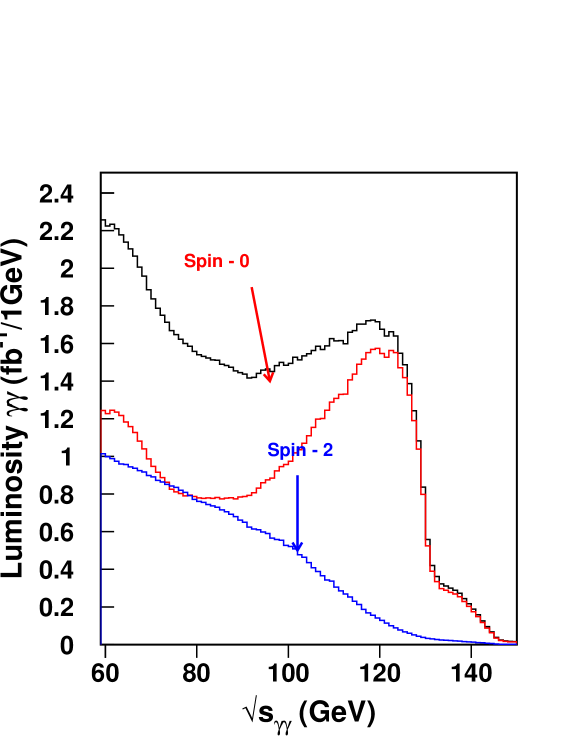
Figure 1: Luminosity spectra for the spin of the two colliding photons $J_{z}$ = 0 and $J_{z}$ = 2.

It depends strongly on the differential luminosity, $\frac{d{\cal L}_{\gamma\gamma}}{\rm d\sqrt{s}_{\gamma\gamma}}|_{M_{\rm H}}$. The shape of the luminosity distribution depends on the electron and laser beam parameters. The electron and laser beam energy considered for this study are 105 GeV and 1 eV, respectively, resulting in the maximum photon energy of about 75 GeV, suitable to study a Higgs boson with the mass of 120 GeV. The combination of the polarisation of the laser and the electron are chosen such to make the generated photon spectrum peak at its maximum energy. The helicity combination of the two high energy photons is arranged such that $J_{\rm z}$ = 0 state is dominant. The luminosity distributions for the $J_{\rm z}$=0 and $J_{\rm z}$ = 2 are provided by the CIRCE2 [4] program and shown in Figure 1. Beamstrahlung, secondary collisions between electrons and laser beam photons, and other non-linear effects are taken into account when calculating the $\gamma\gamma$ luminosity. The resulting value of $\frac{d{\cal L}_{\gamma\gamma}}{\rm d\sqrt{s}_{\gamma\gamma}}|_{M_{\rm H}}$ is 1.6 fb^-1/GeV.

The branching ratios BR(H $\to\gamma\gamma$), BR(H $\to\rm b\bar{\rm b}$) and the total width are taken to be 0.22$\%$, 68$\%$ and 4 MeV, respectively, and are calculated with the HDECAY [5] program including QCD radiative corrections. A signal rate of about 20000 events per year can be achieved under these conditions.

The main background processes are the direct continuum $\gamma\gamma\to\rm b\bar{\rm b}$ and $\gamma\gamma\to\rm c\bar{\rm c}$ production. Due to helicity conservation, the continuum background production proceeds mainly through the states of opposite photon helicities, making the states $J_{\rm z}=2$. Choosing equal helicity photon polarisations the cross section of the continuum background is suppressed by a factor $M_{\rm q}^{2}/s_{\gamma\gamma}$, with $M_{\rm q}$ being the quark mass. Unfortunately, this suppression does not apply to the process $\gamma\gamma\to\rm q\bar{\rm q}\rm g$, because after the gluon radiation the $\rm q\bar{\rm q}$ system is not necessarily in a $J_{\rm z}=0$ state. The surviving background is large and overwhelms the signal.

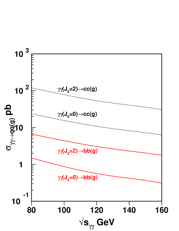
Figure 2: Cross sections for the $\gamma\gamma\to\rm b\bar{\rm b}(\rm g)$ and $\gamma\gamma\to\rm c\bar{\rm c}(\rm g)$ processes including QCD radiative corrections for $J_{z}$ = 0 and $J_{z}$ = 2.

The signal $\gamma\gamma\to{\rm H}\to{\rm b}\bar{\rm b}$ process, as well as the background $\gamma\gamma\to{\rm q}\bar{\rm q}$(g) events are generated with the PYTHIA [6] program. Parton evolution and hadronization are simulated using the parton shower and the string fragmentation models. A convolution with the luminosity distribution is performed, and kinematic cuts of $|\cos\theta|<0.9$ and $\sqrt{s}_{\gamma\gamma}$ greater than 80 GeV are imposed during the event generation, $\theta$ denoting the polar angle of the produced quarks. The QCD corrections to $\gamma\gamma\to{\rm q}\bar{\rm q}$ have to be taken into account for a reliable background estimation. For this purpose we use the total cross sections shown in Figure 2, which include the soft and hard gluon emission [7], virtual corrections [7] and non-Sudakov form factors [8] to weight the event. The event topology is given by the parton shower model.

The effective cross sections, the number of expected and generated signal and background events are presented in Table 1.

To simulate the response of the apparatus we use SIMDET [9], a fast Monte Carlo program which smears the kinematics of the particles in the final state according to the detector resolutions. The detector used in the simulation follows the proposal presented in the Technical Design Report of the TESLA $\rm e^{+}\rm e^{-}$ Linear Collider [10]. However, the changes in the detector design for $\gamma\gamma$ collisions will affect only the forward region [11] which is not important for this analysis.

Event selection

The analysis aims to select events with two or three multiplicity jets from the Higgs boson decay. Two of these jets contain bottom quarks. The invariant mass of the jets has to be consistent with the Higgs mass.

Jets are reconstructed using the DURHAM clustering scheme [12] with the parameter y_cut=0.02.

We select events with a visible energy larger than 95 GeV and the energy imbalance longitudinal to the beam direction below 10$\%$ of the visible energy. Figures 3a,b shows the distribution of the cosine of the thrust angle for the signal and background events. The s-channel signal process has an isotropic angular distribution, while the t-channel background processes are forward peaked. We require the absolute value of this quantity to be below 0.7.

The cross section for the continuum production of the charm quark is 16 times larger than for bottom quarks, therefore b-quark tagging is crucial in this analysis. The b-tagging algorithm relies on a neural network with 12 inputs and 3 output nodes, described in Ref. [13]. The most important inputs comprise the impact parameter joint probability tag introduced by ALEPH [14], the $p_{t}$ corrected vertex invariant mass obtained with the ZVTOP algorithm written for the SLD experiment [15] and a one-prong charm tag using the largest and second largest track impact parameter significances in $r$ - $\phi$ and $r$ - $z$, in jets where ZVTOP found only the primary vertex. The spectrum of the neural network output $NN_{\rm out}$ to discriminate b-quark jets from u-, d-, s- and c-quark jets is presented in Figure 4a. The performance of the neural network b-tag in Z⁰ decays is shown in Figure 4b. We require at least 2 vertices to be found and ask that the $NN_{\rm out}$ to be greater than 0.95. The b-tagging efficiency is 70$\%$ and corresponds to a purity of 98$\%$.

The efficiency of this selection is found to be 36$\%$.

Discussion of the QCD $\gamma\gamma\to{\rm hadrons}$ background

A background not discussed yet is the process $\gamma\gamma\to$hadrons, where photons interact hadronically at the interaction point. With a total hadronic cross section in $\gamma\gamma$ collisions of 400 nb, we estimate about 1.4 such events per bunch crossing. These events obscure the interesting physics processes described in the previous sections. For this reason this class of events needs to be included in the PYTHIA simulation for overlap. The HADES [16] program is used for this purpose. A large fraction of this background is distributed at small angles and we believe that it can be reduced cutting on the polar angle of the tracks [17]. A careful study of this hadronic background is currently being performed.

Results

The reconstructed invariant mass for the selected signal and background events is shown in Figure 5. To enhance the signal a cut on the invariant mass is tuned such that the statistical significance of the signal over background is maximised. Events in the mass region of 106 GeV $<M_{jj}<$ 126 GeV are selected. The number of estimated signal and background events in this window are 6018 and 7111, respectively.

The two photon decay width of the Higgs boson is proportional to the event rates of the Higgs signal. The statistical error of the number of signal events, $\sqrt{N}_{\rm obs}/({\it N}_{\rm obs}-{\it N}_{\rm bkg})$, corresponds to the statistical error of this measurement. Here $N_{\rm obs}$ is the number of observed events, while $N_{\rm bkg}$ is the number of expected background events.

We obtain

$$\frac{\Delta[\Gamma(\rm H\to\gamma\gamma)\times\rm BR(\rm H\to\rm b\bar{\rm b})]}{[\Gamma(\rm H\to\gamma\gamma)\times\rm BR(\rm H\to\rm b\bar{\rm b})]}=\sqrt{N}_{\rm obs}/({\it N}_{\rm obs}-{\it N}_{\rm bkg})=1.9\%.$$

We can improve this number by 0.1$\%$ doing a fit with the function

$$\chi^{2}=\Sigma\frac{((f_{i}N_{\rm H}+b_{i})^{2}-d_{i}^{2})^{2}}{d_{i}},$$

with $f_{i}=\frac{s_{i}}{s}$ being the fraction of signal events, $b_{i}$ and $d_{i}$ the background and observed number of events in each bin of the invariant mass distributins and $N_{\rm H}$ a fit parameter.

We conclude that for a Higgs boson with a mass $M_{\rm H}$=120 GeV we can measure the product $\Gamma(\rm H\to\gamma\gamma)\times\rm BR(\rm H\to\rm b\bar{\rm b})$ with an accuracy of 1.8$\%$ using an integrated luminosity corresponding to one year of data taking at the TESLA Photon Collider.

	Cross section	Number of	Number of
	(pb)	expected events	generated events
Signal process	$\sigma_{\rm eff}$, ${\cal L}$ = 80 fb-1	20000	50000
$\gamma\gamma\to\rm H\to{\rm b}\bar{\rm b}$	0.25
Background
$\gamma\gamma\to{\rm b}\bar{\rm b}$(g)	0.75	44175.0	600000
$J$ = 0		(${\cal L}_{J=0}=58.9$ fb-1)
$\gamma\gamma\to{\rm b}\bar{\rm b}$(g)	4.79	102314.4	600000
$J$ = 2		(${\cal L}_{J=2}=21.1$ fb-1)
$\gamma\gamma\to{\rm c}\bar{\rm c}$(g)	13.4	789260.0	600000
$J$ = 0
$\gamma\gamma\to{\rm c}\bar{\rm c}$(g)	85.1	1817734.0	600000
$J$ = 2

Table 1: Cross sections and the number of expected and generated events for the signal and background processes.

Figure 3: Distributions for the cosine of the thrust angle for signal a) and background b) events.

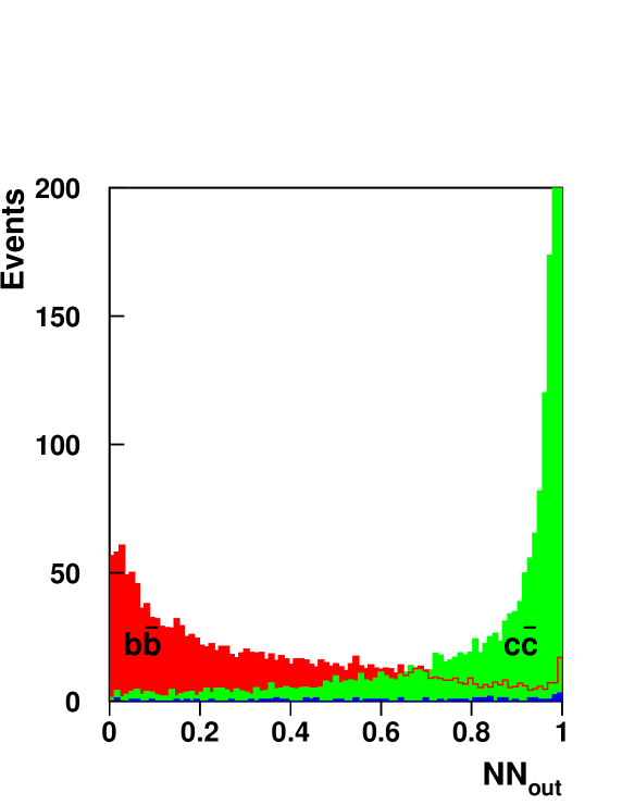
Figure 4: a) Distribution of the neural network output and b) efficiency versus purity curve for the neural network based b-tag in Z⁰ decays.

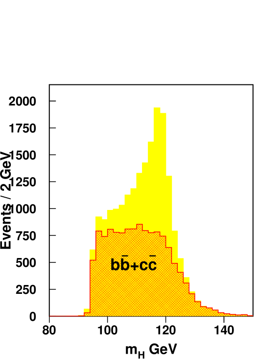
Figure 5: Distribution of the reconstructed invariant mass for the signal and background events.

References

- [1] D.L. Borden, D.A. Bauer and D.O. Caldwell, Phys. Rev. D48 (1993) 4018.
- [2] B. Badelek et al., TESLA Technical Design Report Part VI, Chapter I: The Photon Collider at TESLA, DESY-01-011.
- [3] T. Ohgaki, T. Takahashi and I. Watanabe, hep-ph/9703301; G. Jikia and S. Söldner-Rembold, Nucl. Inst. and Meth A472 (2001) 133; P. Niezurawski, A.F. Zarnecki and M. Krawczyk, Acta Physica Polonica B34 (2003) 177. P. Niezurawski, A.F. Zarnecki and M. Krawczyk, hep-ph/0307183.
- [4] V.I. Telnov, A Code for the Simulation of Luminosities and QED Backgrounds at Photon Colliders, talk presented at the 2nd ECFA/DESY Workshop on Physics and Detectors for a 90-800 GeV Linear Collider, St. Malo, France, April 2002. T. Ohl, Circe Version 2.0: Beam Spectra for Simulating Linear Collider and Photon Collider Physics, ftp://heplix.ikp.physik.tu-darmstadt.de/pub/ohl/circe2/doc/manual.pdf.
- [5] A. Djouadi, J. Kalinowski and M. Spira, Comp. Phys. Comm. 108 (1998) 56.
- [6] T. Sjöstrand, CERN-TH/7112/93 (1993), revised August 1995; T. Sjöstrand, Comp. Phys. Comm. 82 (1994) 74.
- [7] G. Jikia and A. Tkabladze, Phys. Rev. D54 (1996) 2030.
- [8] M. Melles and W.J. Stirling, Phys. Rev. D59 (1999) 94009; M. Melles and W.J. Stirling, Eur. Phys. J. C9 (1999) 101.
- [9] M. Pohl and H.J. Schreiber, DESY-02-061, hep-ex/0206009.
- [10] J.A. Aguilar-Saavedra et al., TESLA Technical Design Report Part IV: A detector for TESLA, DESY-01-011.
- [11] K. Mönig, private communication.
- [12] S. Bethke et al., Nucl. Phys. B370 (1992) 310.
- [13] R. Hawkings, LC-PHSM-2000-021.
- [14] D. Buskulic et al. [ALEPH Collaboration], Phys. Lett. B313 (1993) 535.
- [15] D.J. Jackson, Nucl. Instr. Meth. A388 (1997) 247.
- [16] D. Schulte, http://clicphysics.web.cern.ch/CLICphysics/.
- [17] A. Rosca, talk presented at the 3rd ECFA/DESY Workshop on Physics and Detectors for a 90-800 GeV Linear Collider, Prague, Czech Republic, November 2002.