CJK- Improved LO Parton Distributions in the Real Photon and Their Experimental Uncertainties

Abstract

A new analysis of the radiatively generated, LO quark ($u,d,s,c,b$) and gluon densities in the real, unpolarized photon, improved in respect to our paper [1], is presented. We perform four new global fits to the experimental data for $F_{2}^{\gamma}$, two using a standard FFNS approach and two based on ACOT_χ scheme [2], leading to the FFNS_CJK and CJK models. We also present the analysis of the uncertainties of the new CJK 2 parton distributions due to the experimental errors, the very first such analysis performed for the photon. This analysis is based on the Hessian method, for a comparison for chosen cross-sections we use also the Lagrange method.

1 Introduction

We continue our LO analysis [1] of the parton distributions in the unpolarized real photon, which led us to a construction of the CJKL parton parametrization, improving and broadening our investigation. Like previously our aim is to develop a proper description of the heavy charm- and bottom-quark contributions to the photon structure function, $F_{2}^{\gamma}(x,Q^{2})$. The new models FFNS_CJK 1 and CJK 1 are slightly modified versions of our previous FFNS_CJKL and CJKL models, respectively. In addition we analyse the FFNS_CJK 2 model, which includes the so-called “resolved-photon” contribution of heavy quarks to $F_{2}^{\gamma}(x,Q^{2})$ , given by the $\gamma^{*}G\to h\bar{h}$ process, and CJK 2 model, with an improved positivity constraint. All models are based on the idea of radiatively generated parton distributions introduced by the GRV group (see e.g. [3]).

In this analysis we neglect TPC2$\gamma$ data, as in other recent analyses, and slightly modify, with respect to previous analysis, both types of models. Moreover, for the very first time for the photon, we estimate uncertainties of the parton distributions due to the experimental errors of data. Following the analyses of this type performed for proton structure by the CTEQ Collaboration, [4]–[6] and the MRST group, [7] we use the Hessian method to obtain sets of parton parametrizations allowing, along with the parton parametrization of the best fit, to calculate the best estimate and uncertainty of any observable depending on the parton densities in real photon. We compare our results for $F_{2,c}^{\gamma}$ and prompt photon production in $\gamma\gamma$ obtained with the Hessian and Lagrange ([4],[7], [8]) methods.

2 FFNS_CJK and CJK models

The difference between the FFNS_CJK and CJK models lays in the approach to the calculation of the heavy quark $h$ ($c$ and $b$) contributions to the photon structure function $F_{2}^{\gamma}(x,Q^{2})$. The FFNS_CJK models base on a widely adopted Fixed Flavour Number Scheme in which there are no heavy quarks among partons. They contribute to $F_{2}^{\gamma}(x,Q^{2})$ by a ’direct’ (Bethe-Heitler) $\gamma^{*}\gamma\to h\bar{h}$ process ($F_{2,h}^{\gamma}(x,Q^{2})|_{dir}$), in addition one can also include the so-called ’resolved’-photon contribution from $\gamma^{*}G\to h\bar{h}$ ($F_{2,h}^{\gamma}(x,Q^{2})|_{res}$) [9]:

$$F_{2}^{\gamma}(x,Q^{2})|_{FFNS}=x\sum_{i=1}^{3}e_{i}^{2}(q_{i}^{\gamma}+\bar{q}_{i}^{\gamma})(x,Q^{2})$$ (1)

$$+\sum_{h(=c,b)}^{2}\left[F_{2,h}^{\gamma}(x,Q^{2})|_{dir}+F_{2,h}^{\gamma}(x,Q^{2})|_{res}\right],$$

with $q^{\gamma}_{i}$ ($\bar{q}^{\gamma}_{i}$) being the light $u,d,s$ quark (anti-quark) densities governed by the DGLAP evolution equations.

The CJK models adopt the ACOT_χ scheme [2] which is a recent realization of the Variable Flavour Number Scheme. In this approach heavy quarks are, similarly to the light quarks, constituents of the photon. Therefore, apart from the direct and resolved-photon contributions also $q_{h}$ contribute to $F_{2}^{\gamma}(x,Q^{2})$ . It leads to a double counting of the heavy quark contributions to $F_{2}^{\gamma}(x,Q^{2})$ , therefore inclusion of the corresponding subtraction terms, $F_{2,h}^{\gamma}|_{\mathrm{dir},\mathrm{sub}}$ and $F_{2,h}^{\gamma}|_{\mathrm{res},\mathrm{sub}}$, is necessary.

Next, following the ACOT_χ approach, we use the $\chi_{h}$ parameters to obtain the proper vanishing of the heavy-quark densities below the kinematic thresholds, for DIS given by the $W^{2}=Q^{2}(1-x)/x=4m_{h}^{2}$. Substitution of $x$ with $\chi_{h}=x(1+4m_{h}^{2}/Q^{2})$ in $q_{h}$ and in subtraction terms should lead to the correct threshold behaviour as $\chi_{h}\to 1$ for $W\to 2m_{h}$. In the CJK models

$$F_{2}^{\gamma}(x,Q^{2})|_{CJK}=\sum_{i=1}^{3}xe_{i}^{2}(q_{i}^{\gamma}+\bar{q}_{i}^{\gamma})(x,Q^{2})$$ (2)

$$+\sum_{h(=c,b)}^{2}xe_{h}^{2}(q_{h}^{\gamma}+\bar{q}_{h}^{\gamma})(\chi_{h},Q^{2})$$

$$+\sum_{h(=c,b)}^{2}\left[F_{2,h}^{\gamma}(x,Q^{2})|_{dir}+F_{2,h}^{\gamma}(x,Q^{2})|_{res}\right]$$

$$-\sum_{h(=c,b)}^{2}\left[F_{2,h}^{\gamma}|_{\mathrm{dir},\mathrm{sub}}+F_{2,h}^{\gamma}|_{\mathrm{res},\mathrm{sub}}\right].$$

The QCD evolution (DGLAP) starts from a scale chosen to be small, $Q_{0}^{2}=0.25$ GeV², for both types of models, hence our parton densities are radiatively generated. As it is well known the point-like solutions of the evolution equations are calculable without further assumptions, while the hadronic parts need the input distributions. For this purpose we utilize the Vector Meson Dominance (VMD) model, assuming

$$f_{had}^{\gamma}(x,Q_{0}^{2})=\sum_{V}\frac{4\pi\alpha}{\hat{f}^{2}_{V}}f^{V}(x,Q_{0}^{2})=\kappa\frac{4\pi\alpha}{\hat{f}^{2}_{\rho}}f^{\rho}(x,Q_{0}^{2}),$$ (3)

where the sum over all light vector mesons (V) is proportional to the $\rho^{0}$-meson parton density with a parameter $\kappa$. We take the input densities of the $\rho$ meson at $Q_{0}^{2}$ in the form of valence-like distributions both for the (light) quarks ($v^{\rho}$) and gluons ($G^{\rho}$):

$$xv^{\rho}(x,Q_{0}^{2}) = N_{v}x^{\alpha}(1-x)^{\beta},$$ (4)

$$xG^{\rho}(x,Q_{0}^{2}) = \tilde{N}_{g}xv^{\rho}(x,Q_{0}^{2})=N_{g}x^{\alpha}(1-x)^{\beta},$$

$$x\zeta^{\rho}(x,Q_{0}^{2}) = 0,$$

where $N_{g}=\tilde{N}_{g}N_{v}$. All sea-quark distributions (denoted as $\zeta^{\rho}$), including $s$-quarks, are neglected at the input scale. The valence-quark and gluon densities satisfy the constraint representing the energy-momentum sum rule for $\rho$:

$$\int_{0}^{1}x(2v^{\rho}(x,Q_{0}^{2})+G^{\rho}(x,Q_{0}^{2}))dx=1.$$ (5)

One can impose an extra constraint related to the number of valence quarks:

$$n_{v}=\int_{0}^{1}2v^{\rho}(x,Q_{0}^{2})=2.$$ (6)

Use of both constraints allows to express $N_{v}$ and $N_{g}$ in terms of $\alpha$, $\beta$ and $\kappa$, reducing the number of free parameters to three.

3 New analysis

In our new analysis we improve treatment of the running of $\alpha_{s}$ by differentiating the number of active quarks in the running of $\alpha_{s}$ and in the evolution equations, and by using lower values of $\Lambda_{QCD}$. We first describe new aspects of our analysis which are common to all considered models.

3.1 Data

New fits were performed using all, $F_{2}^{\gamma}(x,Q^{2})$ data, except the old TPC$\gamma$. In our former global analysis [1] we used 208 $F_{2}^{\gamma}(x,Q^{2})$ experimental points. Now we decided to exclude the TPC2$\gamma$ data (as for instance in [10]) since these data are considered to be not in agreement with other measurements. After the exclusion we have 182 data points.

3.2 $\alpha_{s}$ running and values of $\Lambda^{(N_{q})}$

The running of the strong coupling constant at lowest order is given by the well-known formula:

$$\alpha_{s}^{(N_{q})}(Q^{2})=\frac{4\pi}{\beta_{0}\ln(Q^{2}/\Lambda^{{(N_{q})}^{2}})},\;\beta_{0}=11-\frac{2}{3}N_{q},$$ (7)

where $\Lambda^{(N_{q})}$ is the $\Lambda_{QCD}$ value for $N_{q}$ quarks. $N_{q}$ increases by one whenever $Q^{2}$ reaches a heavy quark threshold, i.e. when $Q^{2}=m_{h}^{2}$. The condition $\alpha_{s}^{(N_{q})}(m_{h}^{2})=\alpha_{s}^{(N_{q}+1)}(m_{h}^{2})$ is imposed in order to ensure the continuity of the strong coupling constant. In the new analyses we introduce the number of active quarks in the photon, denoted by $N_{f}$, which differs from the number of quarks contributing to the running of $\alpha_{s}$.

The distinction between both numbers of quarks forces to use slightly more complicated formulae for the evolution of the parton densities than in our previous analysis. More precisely, we must proceed in three steps to perform the DGLAP evolution. In the first step, describing the evolution from the input scale $Q_{0}$ to the charm-quark mass $m_{c}$, the hadronic input $q_{\mathrm{had}}^{\gamma}(x,Q_{0}^{2})$ is taken from the VMD model. In the second step we evolve the parton distributions from $m_{c}$ to the beauty-quark mass, $m_{b}$, a new hadronic input is given by the sum of already evolved hadronic and point-like contributions to the parton density. The point-like distribution at $Q^{2}=m_{c}^{2}$ becomes zero again. The same is repeated for $Q^{2}>m_{b}^{2}$. That way we can solve the equations for three ranges of $Q^{2}$, in which $N_{f}=3,4$ and 5, separately. In each range values of $b_{0}$ and $\Lambda$ depend on $N_{q}$.

In the previous work we assumed (following the GRV group approach [3]) that the LO and NLO $\Lambda$ values for four active flavors are equal, and used $\Lambda^{(4)}=280$ MeV from the Particle Data Group (PDG) report [11]. We now abandon this assumption and take for $\Lambda^{(4)}=115$ MeV, which is obtained in LO from the world average value $\alpha_{s}(M_{Z})=0.117$, with $M_{Z}=91.188$ GeV, using Eq. 7. Imposing the continuity condition for the strong coupling constant and $m_{c}=1.3$ GeV and $m_{b}=4.3$ GeV, we obtain $\Lambda^{(3)}=138$ MeV and $\Lambda^{(5)}=84$ MeV.

3.3 VDM

In our new analysis we try to relax the constraint on $n_{v}$ (6). This leads to 4-parameter fit.

3.4 FFNS

In the FFNS_CJK 2 model we include the so-called “resolved-photon” contribution of heavy quarks to $F_{2}^{\gamma}(x,Q^{2})$ , given by the $\gamma^{*}G\to h\bar{h}$ process.

3.5 Subtraction terms in CJK models

In [1] we derived the subtraction term for a direct contribution, $F_{2,h}^{\gamma}|_{dir,subtr}$, from the integration up to $Q^{2}$ of a part of the DGLAP evolution equations, namely:

$$\frac{dq_{h}^{\gamma}(x,Q^{2})}{d\ln Q^{2}}=\frac{\alpha}{2\pi}e_{h}^{2}k(x),$$ (8)

where $k(x)$ is the lowest order photon-quark splitting function (see Eq. (7) in Ref. [1]). For the lower limit we took in Ref. [1] the natural for a Bethe-Heitler process limit $Q^{2}_{low}=m_{h}^{2}$. However, since the threshold condition is $W^{2}\geq 4m_{h}^{2}$, even for $Q^{2}<m_{h}^{2}$ the heavy-quark contributions do not vanish as long as the condition $x<Q^{2}/(Q^{2}+4m_{h}^{2})$ is fulfilled. In this paper we take $Q^{2}_{low}=Q^{2}_{0}$, which improves quality of the fits. The direct subtraction term has now the form:

$$F_{2,h}^{\gamma}|_{dir,subtr}(x,Q^{2})=x\ln\frac{Q^{2}}{Q_{0}^{2}}3e_{h}^{4}\frac{\alpha}{\pi}(x^{2}+(1-x)^{2}).$$ (9)

We apply the same change to the subtraction term for the resolved-photon contribution:

$$F_{2,h}^{\gamma}|_{res,subtr}=x\ln\frac{Q^{2}}{{Q^{2}_{0}}}e_{h}^{2}\frac{\alpha_{s}(Q^{2})}{\pi}\int_{x}^{1}\frac{dy}{y}P_{qG}(\frac{x}{y})G^{\gamma}(y,Q^{2}).$$ (10)

As we noticed in Section 2 the $x\to\chi_{h}$ substitution leads to the proper threshold behavior of all the heavy-quark contributions to the $F_{2}^{\gamma}(x,Q^{2})$, except for both subtraction terms. This is already seen in Eq. (9) that this term does not vanish for $\chi_{h}\to 1$ and therefore by subtracting it the resulting heavy-quark contribution to $F_{2}^{\gamma}$ may become negative for large $x$. An extra constraint to avoid this unphysical situation is, thus, needed. In Ref. [1] we imposed the simple condition (positivity constraint) that the heavy quark contribution to $F_{2}^{\gamma}(x,Q^{2})$ has to be positive. Unfortunately, this constraint was not strong enough and for some small windows at small and large $x$ the still unphysical situation $F_{2,h}^{\gamma}(x,Q^{2})<F_{2,h}^{\gamma}(x,Q^{2})|_{direct}+F_{2,h}^{\gamma}(x,Q^{2})|_{resolved}$ was found [12]. In this paper we apply new condition:

$$F_{2,h}^{\gamma}(x,Q^{2})\geq F_{2,h}^{\gamma}(x,Q^{2})|_{dir}+F_{2,h}^{\gamma}(x,Q^{2})|_{res}.$$ (11)

4 Results of the new $F_{2}^{\gamma}$ global fits

In the fits we use 182 $F_{2}^{\gamma}(x,Q^{2})$ experimental points with equal weights. Fits based on the least-squares principle (minimum of $\chi^{2}$) were done using Minuit [13]. Systematic and statistical errors on data points were added in quadrature.

The CJK 1 and 2 models differ in the form of the positivity constraint. In the CJK 1 model we keep the old condition $F_{2,h}^{\gamma}(x,Q^{2})>0$ while the CJK 2 model imposes the condition (11). In these models we do not apply the sum rule (6) and have four free parameters: $\alpha,\beta,N_{v},\kappa$ related to the initial quark and gluon densities at the scale $Q^{2}_{0}=0.25$ GeV² (2).

The two FFNS models differ by the resolved-photon contribution of heavy quarks to $F_{2}^{\gamma}(x,Q^{2})$. It appears only in the FFNS_CJK 2 model. In both FFNS models we impose constraints (5) and (6). That allows to write $N_{v}$ in terms of $\alpha$, $\beta$ and $\kappa$ reducing the number of free parameters to three .

The results for the total $\chi^{2}$ for 182 points and the $\chi^{2}$ per degree of freedom for our new fits are presented in table 1. The fitted values for parameters $\alpha$, $\beta$, $\kappa$ and $N_{v}$ are also presented together with the errors obtained from Minos program with the standard requirement of $\Delta\chi^{2}=1$. In the case of the FFNS_CJK models the $N_{v}$ parameter is calculated from the constraint (5) and therefore we do not state its error. Note, that the valence number integral $n_{v}$ (6) gives in CJK models 1.94 and 2.00, for CJK 1 and CJK 2, respectively.

model		$\chi^{2}$ (182 pts)	$\chi^{2}/_{\rm DOF}$		$\kappa$	$\alpha$	$\beta$	$N_{v}$		$\tilde{N}_{g}$
FFNSCJK 1		314.0	1.754		$2.267^{+0.063}_{-0.072}$	$0.265^{+0.038}_{-0.032}$	$0.792^{+0.189}_{-0.149}$	0.358		5.02
FFNSCJK 2		279.8	1.563		$2.110^{+0.084}_{-0.090}$	$0.310^{+0.054}_{-0.051}$	$0.823^{+0.265}_{-0.223}$	0.415		4.51
CJK 1		273.9	1.539		$2.146^{+0.154}_{-0.144}$	$0.218^{+0.070}_{-0.063}$	$0.462^{+0.261}_{-0.227}$	$0.269^{+0.076}_{-0.059}$		5.00
CJK 2		273.7	1.537		$1.934^{+0.131}_{-0.124}$	$0.299^{+0.077}_{-0.069}$	$0.898^{+0.316}_{-0.275}$	$0.404^{+0.116}_{-0.088}$		4.93

Table 1: The total $\chi^{2}$ for 182 data points and per the degree of freedom, and parameters of the best fits for FFNS_CJK and CJK models. Errors are obtained from Minos with $\Delta\chi^{2}=1$.

The $\chi^{2}$ per degree of freedom obtained in our new fits, between 1.5 and 1.7, is better than the old results, mostly due to much lower $\Lambda^{(N_{q})}$ as well as due to modification of the subtraction contributions in the CJK models. The old $\chi^{2}/_{\rm DOF}$ for the same set of 182 data points read 1.99 in the $FFNS_{CJKL}$ and 1.80 in the CJKL model .

We observe that the only real difference in $\chi^{2}/_{\rm DOF}$ is between the first and other three fits and is a result of inclusion or not of the $\gamma^{*}G\to h\bar{h}$ contribution to $F_{2}^{\gamma}(x,Q^{2})$. It is obvious that taking this process into account improves the agreement between model and data.

In light of these results one can conclude that in both, so different treatment of heavy-quark contributions to the photon structure function, all fitted parameters are similar. This is related to the fact, that we use in global fits only data for $F_{2}^{\gamma}$, quantity dominated by the light-quark contributions.

4.1 Comparison with the $F_{2}^{\gamma}$ data

The FFNS_CJK 2 and both CJK models predict a much steeper behaviour of the $F_{2}^{\gamma}(x,Q^{2})$ at small $x$ with respect to FFNS_CJK 1 fit and GRS LO [14] and SaS1D [15] parametrizations. On the other hand these curves are less steep than the FFNS_CJKL and CJKL results from [1]. In the region of $x\gtrsim 0.1$, the behaviour of the $F_{2}^{\gamma}(x,Q^{2})$ obtained from all fits and parametrizations apart from the CJK 1 model is similar. The shape of the CJK 1 fit at high $x$ is a result of the $F_{2,h}^{\gamma}(x,Q^{2})>0$ condition which allows for $F_{2,h}^{\gamma}(x,Q^{2})<F_{2,h}^{\gamma}(x,Q^{2})|_{direct}+F_{2,h}^{\gamma}(x,Q^{2})|_{resolved}$. It effects in the lower position of the characteristic point at which the charm-quark contributions to the $F_{2}^{\gamma}(x,Q^{2})$ appear as compared to other models predictions. Apart from that the CJK 1 fit gives smaller $F_{2}^{\gamma}(x,Q^{2})$ values around this charm-quark threshold. Finally at high $Q^{2}$ and high $x$ the CJK 1 model produces much lower structure function values than all other fits and parametrizations predict. We found that the FFNS_CJK 1 fit gives very similar prediction to the GRS LO parametrization results in the whole range of $x$.

Figure 1 presents the predictions for $F_{2}^{\gamma}(x,Q^{2})$, averaged over medium $x$ regions, compared with the recent OPAL data [16], not used directly in our analysis. Like in our previous analysis we see that all FFNS type predictions (including GRS LO and SaS1D parametrizations) are similar and fairly well describe the experimental data. The CJK models alike the CJKL model gives slightly better agreement with the data.

4.2 Parton densities

The parton densities obtained in the CJK and FFNS_CJK models are all very similar. Of course there are no heavy-quark distributions in FFNS models. In case of the CJK models the $c^{\gamma}(x,Q^{2})$ and $b^{\gamma}(x,Q^{2})$ densities vanish not at $x=1$, as for the GRV LO and SaS1D parametrizations, but at the kinematical threshold, which was our aim. We notice that our new parton densities have all similar shapes but slightly higher values than the corresponding old CJKL distributions. In case of the gluon density we find that all new curves are much steeper than the predictions of the old models and the GRV LO and SaS1D parametrizations, see also below.

4.3 Comparison with $F^{\gamma}_{2,c}$

In Fig. 2 we present our predictions for the $F_{2,c}^{\gamma}$, in comparison with OPAL data [17], not used directly in the analysis, and results of the GRS LO and SaS1D parametrizations.

All our models containing the resolved-photon contribution (FFNS_CJK 2 and both CJK models) agree better with the low $x$ experimental point than other predictions. The GRS LO and SaS1D parametrizations also include the resolved-photon term but in their case the gluon density increased less steep than our models predict, as was already mentioned. Their $F_{2,c}^{\gamma}$ lines lie below results of our new fits but higher than the FFNS_CJK 1 curve which is given solely by the direct Bethe-Heitler contribution.

The CJK models overshoot the experimental point at high $x$ while other predictions agree with it within its uncertainty bounds. Again the $F_{2,c}^{\gamma}$ from the CJK 1 fit vanishes at lower $x$ than in other models.

5 Uncertainties of the parton distributions

Following the corresponding analyses for the proton we consider the experimental uncertainties of the CJK parton densities. This is first analysis of this type for the photon, details are described in [18].

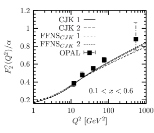
Figure 1: Comparison of the recent OPAL data [16] for the $Q^{2}$-dependence of the averaged over $0.1<x<0.6$ $F_{2}^{\gamma}/\alpha$ with the predictions of the CJK and FFNS_CJK models.

Figure 2: Comparison of the structure function $F_{2,c}^{\gamma}(x,Q^{2})/\alpha$ calculated in the CJK and FFNS_CJK models and in GRS LO [14] and SaS1D [15] parametrizations with the OPAL data [17].

5.1 The Hessian method

The CTEQ Collaboration [4]-[6], developed and applied an improved method of the treatment of the experimental data errors. Later the same formalism has been applied by the MRST group in [7]. The method bases on the Hessian formalism and as a result one obtains a set of parametrizations allowing for the calculation of an uncertainty of any physical observable depending on the parton densities.

We apply the method as described in Refs. [4] and [5]. For the sake of clearness of our procedures we will partly repeat it here keeping the notation introduced by the CTEQ Collaboration.

Let us consider a global fit to the experimental data based on the least-squares principle performed in a model, being parametrized with a set of $\{a_{i},i=1,2,\cdots d\}$ parameters. Each set of values of these parameters constitutes a test parametrization $S$. The set of the best values of parameters $\{a_{i}^{0}\}$, corresponding to the minimal $\chi^{2}$, $\chi_{0}^{2}$, is denoted as $S^{0}$ parametrization. In the Hessian method one makes a basic assumption that the deviation of the global fit from $\chi_{0}^{2}$ can be approximated in its proximity by a quadratic expansion in the basis of parameters $\{a_{i}\}$

$$\Delta\chi^{2}=\chi^{2}-\chi_{0}^{2}=\sum_{i=1}^{d}\sum_{j=1}^{d}H_{ij}(a_{i}-a_{i}^{0})(a_{j}-a_{j}^{0}),$$ (12)

where $H_{ij}$ is an element of the Hessian matrix, calculated as

$$H_{ij}=\frac{1}{2}\left(\frac{\partial^{2}\chi^{2}}{\partial a_{i}\partial a_{j}}\right)_{a_{0}}.$$ (13)

Since the $H_{ij}$ is a symmetric matrix, it has a complete set of $k=1,2...d$ orthonormal eigenvectors $(v_{i})_{k}$ defined by

$$\sum_{j=1}^{d}H_{ij}(v_{j})_{k} = \epsilon_{k}(v_{i})_{k},$$ (14)

$$\sum_{i=1}^{d}(v_{i})_{j}(v_{i})_{k} = \delta_{jk},$$ (15)

with $\{\epsilon_{k}\}$ being the corresponding eigenvalues. Variations around the minimum can be expressed in terms of the basis provided by the set of eigenvectors

$$a_{i}-a_{i}^{0}=\sum_{k=1}^{d}s_{k}z_{k}(v_{i})_{k},$$ (16)

where $\{z_{k}\}$ are new parameters describing the displacement from the best fit. The $\{s_{k}\}$ are scale factors introduced to normalize $\{z_{k}\}$ in such a way that

$$\Delta\chi^{2}=\chi^{2}-\chi_{0}^{2}=\sum_{k=1}^{d}z_{k}^{2}.$$ (17)

The above equation means that the surfaces of constant $\chi^{2}$ are spheres in the $\{z_{k}\}$ space. That way the $\{z_{k}\}$ coordinates create a very useful, normalized basis. The $(v_{i})_{k}\equiv v_{ik}$ matrix describes the transformation between this new basis $\{z_{k}\}$ and old $\{a_{i}\}$ basis. The scaling factors $s_{k}$ are equal to $\sqrt{1/\epsilon_{k}}$ in the ideal quadratic approximation (13).

The Hessian matrix can be calculated from its definition in Eq. (13). Such computation meets many practical problems arising from the large range spanned by the eigenvalues $\{\epsilon_{k}\}$, the numerical noise and non-quadratic contributions to $\chi^{2}$. The solution (an iteration procedure) has been given by the CTEQ Collaboration [4].

Having calculated the eigenvectors, eigenvalues and scaling factors we can create a basis of the parametrizations of the parton densities, $\{S_{k}^{\pm}$, $k=1,\cdots,d\}$. Each parametrization corresponds to a $k$-set of ${a_{i}}$ parameters defined by displacements from $a_{i}^{0}$ of a magnitude $t$ “up” or “down” along the corresponding eigenvector direction

$$a_{i}(S_{k}^{\pm})=a_{i}^{0}\pm t\>(v_{i})_{k}s_{k}.$$ (18)

For each $S_{k}^{\pm}$ parametrization $\Delta\chi^{2}=t^{2}$.

The best value of a physical observable $X$ depending on the photon parton distributions is given as $X(S^{0})$. The uncertainty of $X$, for a displacement from the parton densities minimum by $\Delta\chi^{2}=T^{2}$ ($T$ - the tolerance parameter), can be calculated from a very simple expression (a master equation)

$$\Delta X=\frac{T}{2t}\left(\sum_{k=1}^{d}[X(S_{k}^{+})-X(S_{k}^{-})]^{2}\right)^{\frac{1}{2}}.$$ (19)

Note that having calculated $\Delta X$ for one value of the tolerance parameter $T$ we can obtain the uncertainty of $X$ for any other $T$ by simple scaling of $\Delta X$. This way sets of $\{S_{k}^{\pm}\}$ parton densities give us a perfect tool for studying of the uncertainties of other physical quantities. One of such quantities can be the parton densities themselves.

Finally, we can calculate the uncertainties of the $a_{i}$ parameters of the model. According to Eq. (18) in this case $a_{i}(S_{k}^{+})-a_{i}(S_{k}^{-})=2t(v_{i})_{k}s_{k}$ and the master equation gives a simple expression

$$\Delta a_{i}=T\left(\sum_{k=1}^{d}v_{ik}s_{k}\right)^{\frac{1}{2}}.$$ (20)

In practice we observe the considerable deviations from the ideal quadratic approximation of equation (17). To make an improvement we can adjust the scaling factors $\{s_{i}\}$ either to obtain exactly $\Delta\chi^{2}=t^{2}$ at $z_{i}=t$ for each of the $S_{i}^{\pm}$ sets or to get the best average agreement over some $z_{i}$ range (for instance for $z_{i}\leq t$). Below we apply the second approach.

5.1.1 Estimate of the tolerance parameter $T$ for the photon densities

We consider now the value of the tolerance parameter $T$ for the real-photon parton-densities corresponding to the allowed deviation of the global fit from the minimum, $\Delta\chi^{2}=T^{2}$, as described above. In case of an ideal analysis a standard requirement is $\Delta\chi^{2}=1$. Of course this is not a case for a global fit to the $F_{2}^{\gamma}$ data coming from various experiments, and certainly $T$ must be greater than 1. Unfortunately, no strict rules allowing for estimation of the tolerance parameter exist, as discussed in detail in [5] and [8]. We try to estimate the reliable $T$ value in two ways, both applied to the CJK 2 fit only.

First we examine the mutual compatibility of the experiments used in the fit. That gives the allowed $\Delta\chi^{2}$ greater than 22 and the tolerance parameter $T\sim 5$. As a second test we compare the results of our four fits presented in this paper and find the $T$ values for which parton densities predicted by the FFNS and CJK 1 models lie between the lines of uncertainties of the CJK 2 model. These values are large due to the differences between the gluon densities given by the CJK and FFNS models. The $T\sim 5$ when only the CJK 1 and 2 gluon distributions are compared. For quark distributions $T\leq 7$ when we consider all models. Finally we estimate that the tolerance parameter $T$ should lie in the range $5\sim 10$.

5.1.2 Tests of quadratic approximation

For each CJK model we obtained a set of the $\{(v_{i})_{k}\}$ and $\{s_{k}\}$ values, with $i$ and $k=1,\cdots,4$ (since $d=4$ in CJK models). We used the iteration procedure from [4]. Further we adjusted the scaling factors $\{s_{k}\}$ to improve the average quadratic approximation over the $z_{k}\leq 5$ range.

Further we check if the quadratic approximation on which the Hessian method relies is valid in the considered $\Delta\chi^{2}$ range for the CJK 2 model (for the CJK 1 model results are similar). In the left panel of Fig. 3 we present the comparison of the $\chi^{2}$ dependence along each of four eigenvector directions (for the eigenvector $k$ $z_{i}=\delta_{ik}$) with the dependence of the ideal $\Delta\chi^{2}=z_{i}^{2}$ curve. Only the line corresponding to the eigenvector 4 does not agree with the theoretical prediction. Moreover it has a different shape than other lines which results from the scaling adjustment procedure. In the right panel of Fig. 3 an analogous comparison for the five randomly chosen directions in the $\{z_{i}\}$ space is shown. For each of directions $\sum_{k=1}^{d}z_{k}^{2}=z^{2}$ and the ideal curve corresponds to $\Delta\chi^{2}=z^{2}$. In this case we observe greater deviations from the quadratic approximation.

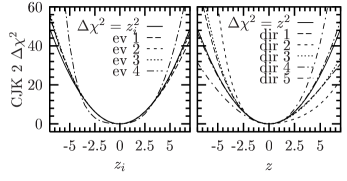
Figure 3: CJK 2 model. The left plot presents a comparison of the $\chi^{2}$ dependence along each of the four eigenvector directions to the ideal $\Delta\chi^{2}=z_{i}^{2}$ curve. In right plot analogous comparison for five random directions in $\{z_{i}\}$ space are shown. The ideal curve corresponds to $\Delta\chi^{2}=\sum z_{i}^{2}=z^{2}$

Figure 4: Parton densities calculated in FFNS_CJK and CJK 1 models compared with the CJK 2 predictions. We plot for $Q^{2}=10$ the $q^{\gamma}(\mathrm{CJK2})/q^{\gamma}(\mathrm{Other})$ ratios of parton densities. Solid lines show the CJK 2 fit uncertainties for $\Delta\chi^{2}=25$.

5.1.3 CJK 1 and CJK 2 parametrizations

The errors calculated within the Hessian quadratic approximation are shown in table 2 for the standard requirement of $\Delta\chi^{2}=1$. They should be compared with the slightly smaller errors calculated by Minuit and shown in table 1.

model	$\kappa$	$\alpha$	$\beta$	$N_{v}$
CJK 1	$2.146^{+0.120}_{-0.107}$	$0.218^{+0.054}_{-0.047}$	$0.462^{+0.157}_{-0.126}$	$0.269^{+0.041}_{-0.035}$
CJK 2	$1.934^{+0.112}_{-0.103}$	$0.299^{+0.061}_{-0.051}$	$0.898^{+0.204}_{-0.156}$	$0.404^{+0.066}_{-0.054}$

Table 2: The parameters of the fits for CJK models with errors calculated in the Hessian quadratic approximation for the standard requirement of $\Delta\chi^{2}=1$

All parton distributions are further parametrized on a grid. The resulting programs can be found on the web-page [19].

5.1.4 Uncertainties of the CJK 2 parton densities

In this section we discuss the uncertainties of the CJK 2 parton densities, the results obtained with CJK 1 model are very similar.

In Figure 4 the up, strange and charm-quark and gluon densities calculated in FFNS_CJK and CJK 1 models are compared with the CJK 2 predictions. We plot the $q^{\gamma}(\mathrm{CJK\>2})/q^{\gamma}(\mathrm{Other\>models})$ ratios of the parton $q^{\gamma}$ densities calculated in the CJK 2 model to their values obtained with other models for $Q^{2}=10$. Solid lines show the CJK 2 fit uncertainties for $\Delta\chi^{2}=25$ computed with the $\{S_{k}^{\pm}\}$ parametrizations.

First we notice that predictions of all our models for all considered parton distributions lie between the lines of the CJK 2 uncertainties. This indicates that the choice of $\Delta\chi^{2}=25$ agrees with the differences among our four models. We found, that the SaS1D results differ very substantially from the CJK 2 ones (not shown).

As expected the up-quark distribution is the one best constrained by the experimental data while the greatest uncertainties are for the gluon densities. In the case of $u^{\gamma}$ the $\Delta\chi^{2}=25$ band widens in the small $x$ region. Alike in the case of $s$- and $c$-quark uncertainties it shrinks at high $x$. On contrary the gluon distributions are least constrained at the region of $x\to 1$. All uncertainties become slightly smaller for higher $Q^{2}$.

5.2 Lagrange method for the uncertainties of the parton distributions

The Hessian method allows the computation of the parton density uncertainties in a very simple and effective way. However, the Hessian method relies on the assumption of the quadratic approximation, which as we have shown in the former section, is not perfectly preserved.

There exist another method called the Lagrange multiplier method which allows to find exact uncertainties independently on the quadratic approximation (for the proton structure used in [4],[7] and [8]). In this approach one makes a series of fits on the quantity

$$F(\lambda,\{a_{i}\})=\chi^{2}(\{a_{i}\})+\lambda X(\{a_{i}\}),$$ (21)

each with a different but fixed value of the Lagrange multiplier $\lambda$. As a result one obtains a set of points $(\chi^{2}(\lambda),X(\lambda)$ which characterize the deviation of the physical quantity $X$ from its best value $X_{0}$, for a corresponding deviation of the structure function global fit from its minimum $\Delta\chi^{2}=\chi^{2}(\lambda)-\chi_{0}$. In each of this constrained (by the $\lambda$ parameter) fits we find the best value of $X$ and the optimal $\chi^{2}$. For $\lambda=0$ we return to the basic fit which gives $\{a_{i}^{0}\}$ parameters and allows to calculate the best $X_{0}$ value. The great advantage of this approach lies in the fact that we do not assume anything about the uncertainties. The large computer time consuming of the process of the whole series of minimalizations is a huge disadvantage of the Lagrange method.

5.3 Examples of cross-section uncertainties in Hessian and Lagrange methods

Finally we made a comparison of the uncertainties obtained for the CJK 2 model in Hessian and Lagrange methods for two physical quantities. For the sake of limitation of the computer time we chose two very simple examples: $F^{\gamma}_{2,c}$ points measured by the OPAL Collaboration [17] and the $\gamma q\to\gamma q$ part of the cross-section for prompt photon production in $\gamma\gamma$. Results for the later case are presented in Fig. 5.

6 Summary

We enlarged and improved our previous analysis [1]. We performed new global fits to the $F_{2}^{\gamma}(x,Q^{2})$ data. Two additional models were analysed. New fits gave $\chi^{2}$ per degree of freedom, 1.5-1.7, about 0.25 better than the old results. All features of the CJKL model, such as heavy-quark distributions, good description of the LEP data on the $Q^{2}$ dependence of the $F_{2}^{\gamma}$ and on $F_{2,c}^{\gamma}$ are preserved. We checked that the gluon densities of our models agree with the H1 measurement of the $G^{\gamma}$ distribution performed at $Q^{2}=74$ GeV² [20], Fig. 6.

An analysis of the uncertainties of the CJK parton distributions due to the experimental errors based on the Hessian method was performed for the very first time for the photon. We constructed sets of test parametrizations for both CJK models. They allow to computate uncertainties of any physical quantity depending on the real photon parton densities.

Parametrization programs for all models can be obtained from the web-page [19].

7 Acknowledgment

This work was partly supported by the European Community’s Human Potential Programme under contract HPRN-CT-2000-00149 Physics at Collider and HPRN-CT-2002-00311 EURIDICE.

Figure 5: CJK 2 model. Lagrange and Hessian method results for the direct resolved (DR) part of the $\gamma\gamma\to\gamma q$ cross-section. The dashed lines represent the 10 to 30% deviation from the Hessian result.

Figure 6: Comparison of the gluon distribution obtained in the H1 measurement performed at $Q^{2}=74$ GeV² [20] with the predictions of the CJK, FFNS_CJK models and GRV LO [3], GRS LO [14] and SaS1D [15] parametrizations with the OPAL measurement [17].

References

- [1] F. Cornet, P. Jankowski, M. Krawczyk and A. Lorca, Phys. Rev. D68 014010 (2003)
- [2] S. Kretzer, C. Schmidt and W. Tung, J. Phys. G28, 983 (2002)
- [3] M. Glück, E. Reya and A. Vogt, Phys. Rev. D46, 1973 (1992)
- [4] J. Pumplin, D.R. Stump and W.K. Tung, Phys. Rev. D65, 014011 (2002)
- [5] J. Pumplin et al., Phys. Rev. D65, 014013 (2002)
- [6] J. Pumplin et al., JHEP 0207, 012 (2002)
- [7] A.D. Martin, R.G. Roberts, W.J. Stirling and R.S. Thorne, Eur. Phys. J. C28, 455 (2003)
- [8] D. Stump et al., Phys. Rev. D65, 014012 (2002)
- [9] M.Glück, E.Reya and M.Stratmann, Phys. Rev. D51, 3220 (1995)
- [10] S. Albino, M. Klasen and S. Söldner-Rembold, Phys. Rev. Lett. 89, 122004 (2002).
- [11] Particle Data Group (D.E. Groom et al.), Eur. Phys. J. C15, 1 (2000)
- [12] We thank Mariusz Przybycień for pointing this problem to us.
- [13] F. James and M. Roos, Comput. Phys. Commun. 10, 343 (1975)
- [14] M. Glück, E. Reya and I. Schienbein, Phys. Rev. D60, 054019 (1999), Erratum-ibid. D62, 019902 (2000)
- [15] G.A. Schuler and T. Sjöstrand, Z. Phys. C68, 607 (1995); Phys. Lett. B376, 193 (1996)
- [16] OPAL Collaboration, G. Abbiendi et al., Phys. Lett. B533, 207 (2002).
- [17] OPAL Collaboration, G. Abbiendi et al., Phys. Lett. B539, 13 (2002)
- [18] P. Jankowski PhD thesis, and F. Cornet, P. Jankowski, M. Krawczyk, in preparation
-
[19]
http://www.fuw.edu.pl/
~pjank/param.html - [20] H1 Collaboration, C. Adloff et al., Phys. Lett. B483, 36 (2000)