Perturbative corrections to curvature sum rules

Abstract

Two new sum rules were recently discovered by Le Yaouanc et al. by applying the operator product expansion to the nonforward matrix element of a time-ordered product of $b\to c$ currents in the heavy-quark limit of QCD. They lead to the constraints $\sigma^{2}>5\rho^{2}/4$ and $\sigma^{2}>3(\rho^{2})^{2}/5+4\rho^{2}/5$ on the curvature of the $\bar{B}\to D^{(*)}$ Isgur-Wise function, both of which imply the absolute lower bound $\sigma^{2}>15/16$ when combined with the Uraltsev bound $\rho^{2}>3/4$ on the slope. This paper calculates order $\alpha_{s}$ corrections to these bounds, increasing the accuracy of the resultant constraints on the physical form factors. The latter may have implications for the determination of $|V_{cb}|$ from exclusive semileptonic $B$ meson decays.

I Introduction

Heavy quark effective theory (HQET) hqet provides a model-independent method of extracting the CKM matrix element $|V_{cb}|$ from exclusive semileptonic $B$ meson decays. The $\bar{B}\to D^{(*)}l\bar{\nu}$ differential decay rates are given by

$$\frac{\mathrm{d}\Gamma}{\mathrm{d}w}(\bar{B}\to D^{*}l\bar{\nu}) = \frac{G^{2}_{F}|V_{cb}|^{2}m_{B}^{5}}{48\pi^{3}}\,r_{*}^{3}(1-r_{*})^{2}\sqrt{w^{2}-1}\,(w+1)^{2}$$

$$\times\left[1+\frac{4w}{w+1}\frac{1-2wr_{*}+r_{*}^{2}}{(1-r_{*})^{2}}\right]\mathcal{F}_{D^{*}}(w)^{2}\ ,$$

$$\frac{\mathrm{d}\Gamma}{\mathrm{d}w}(\bar{B}\to Dl\bar{\nu}) = \frac{G^{2}_{F}|V_{cb}|^{2}m_{B}^{5}}{48\pi^{3}}\,r^{3}(1+r)^{2}(w^{2}-1)^{3/2}\mathcal{F}_{D}(w)^{2}\ ,$$ (1)

where $r_{(*)}=m_{D^{(*)}}/m_{B}$ and $w=v\cdot v^{\prime}$ is the product of the $\bar{B}$ and $D^{(*)}$ four-velocities. Heavy quark symmetry iw relates $\bar{B}\to D^{(*)}l\bar{\nu}$ form factors to the corresponding Isgur-Wise function, with the result $\mathcal{F}_{D^{*}}(w)=\mathcal{F}_{D}(w)=\xi(w)$ in the heavy-quark limit of QCD. Since $\xi(w)$ is absolutely normalized to unity at zero recoil (i.e., $w=1$) iw ; nus ; shif ; luke , experimental data determine $|V_{cb}|$ without recourse to model-specific assumptions.

This procedure has several sources of uncertainty. First, the identity $\mathcal{F}_{D^{(*)}}(1)=1$ receives both perturbative corrections and corrections suppressed by the heavy $b$ and $c$ quark masses. The former are known to order $\alpha_{s}^{2}$ czar , with unknown higher-order corrections likely less than 1%, but the latter depend on four subleading Isgur-Wise functions and have been estimated only with phenomenological models and quenched lattice QCD.

Another source of error is the extrapolation of measured form factors to zero recoil, where the rates vanish. Linear fits of $\mathcal{F}_{D^{(*)}}(w)$ underestimate the zero-recoil value by about 3%, an effect mostly due to the curvature stone . Using non-linear shapes for $\mathcal{F}_{D^{(*)}}(w)$ reduces this error, and therefore constraints on second and higher derivatives at zero-recoil are welcome. Dispersive constraints disper1 ; disper2 relate second and sometimes higher derivatives to the first and are commonly used.

HQET sum rules provide a complementary way of constraining the $\mathcal{F}_{D^{(*)}}(w)$ shapes. New sum rules for the curvature and higher derivatives of the Isgur-Wise function were derived in Refs. ley1 ; ley2 ; ley3 . Equating the result of inserting a complete set of intermediate states in the nonforward matrix element of a time-ordered product of HQET currents with the operator product expansion (OPE) gives a generic sum rule depending on the products of the velocities of the initial, final, and intermediate states. These are denoted respectively by $v_{i}$, $v_{f}$, and $v^{\prime}$ (the intermediate states all have the same velocity $v^{\prime}$ in the infinite-mass limit), and the products are denoted by

$$\begin{array}[]{r @{,} c @{,} l}w_{if}=v_{i}\cdot v_{f}&\quad w_{i}=v_{i}\cdot v^{\prime}&\quad w_{f}=v_{f}\cdot v^{\prime}\,,\end{array}$$ (2)

or generically $w_{x}$. These parameters are constrained to lie within the range ley1

$$w_{i},w_{f},w_{if}\geq 1\ ,\quad w_{i}w_{f}-\sqrt{(w_{i}^{2}-1)(w_{f}^{2}-1)}\leq w_{if}\leq w_{i}w_{f}+\sqrt{(w_{i}^{2}-1)(w_{f}^{2}-1)}\ ,$$ (3)

and differentiating the generic sum rule with respect to them at $w_{x}=1$ (read: $w_{i}=w_{f}=w_{if}=1$) produces a class of sum rules for derivatives of the Isgur-Wise function at zero recoil. The sum rules of Refs. ley1 ; ley2 ; ley3 were derived at tree level in the heavy-quark limit. The present paper includes the order $\alpha_{s}$ corrections to the new sum rules and uses them to derive bounds on the curvatures of $\mathcal{F}_{D^{(*)}}(w)$ including $\alpha_{s}$ and $\Lambda_{\mathrm{QCD}}/m_{c,b}$ corrections. Including these corrections to the heavy-quark limit is important for meaningful comparison with data and dispersive constraints.

II Derivation of the Generic Sum Rule

The derivation of the generic sum rule follows a well-known formalism bigi ; kap ; boyd ; bjo . It begins with the consideration of the time-ordered product of two arbitrary heavy-heavy currents

$$T_{fi}(\varepsilon) = \frac{i}{2m_{B}}\int d^{4}x\ e^{-iq\cdot x}\,\langle B_{f}(p_{f})|\,T\{J_{\!f}(0),J_{i}(x)\}\,|B_{i}(p_{i})\rangle$$ (4)

as a complex function of $\varepsilon=E_{M}-E_{i}-q^{0}$ at fixed $\vec{q}$, where $E_{M}=\sqrt{m^{2}_{M}+|\vec{p}_{i}+\vec{q}\,|^{2}}$ is the minimum possible energy of the charmed hadronic state that $J_{i}$ can create at fixed $\vec{q}$. The currents have the form

$$J_{\!f}(x)=\bar{b}(x)\Gamma_{\!\!f}c(x)\ ,\ J_{i}(y)=\bar{c}(y)\Gamma_{\!i}b(y)$$ (5)

for any Dirac matrices $\Gamma_{\!i,f}$. Only the choices $\Gamma_{\!i,f}={/\hskip-5.29999ptv}_{i,f}$ and $\Gamma_{\!i,f}={/\hskip-5.29999ptv}_{i,f}\gamma_{5}$ are explored here, but in principle others lead to different sum rules. The $B$ states are ground state $\bar{B}$ or $\bar{B}^{*}$ mesons and have the standard relativistic normalization. As in the derivation of the Uraltsev sum rule uraltsev , the initial and final states do not necessarily have the same velocity. Considering the nonforward matrix element of the time-ordered product is a crucial generalization in deriving the new sum rules ley1 .

From Eq. (4) one proceeds by splitting up the two time-orderings and inserting complete sets of intermediate charm states. The result is

$$T_{fi}(\varepsilon) = \frac{1}{2m_{B}}\sum_{X_{c}}(2\pi)^{3}\delta^{3}(\vec{q}+\vec{p}_{i}-\vec{p}_{X_{c}})\frac{\langle B_{f}|J_{\!f}(0)|X_{c}\rangle\langle X_{c}|J_{i}(0)|B_{i}\rangle}{\varepsilon+E_{X_{c}}-E_{M}-i0^{+}}$$ (6)

$$\mbox{}-\frac{1}{2m_{B}}\sum_{X_{\bar{c}bb}}(2\pi)^{3}\delta^{3}(\vec{q}-\vec{p}_{f}+\vec{p}_{X_{\bar{c}bb}})\frac{\langle B_{f}|J_{i}(0)|X_{\bar{c}bb}\rangle\langle X_{\bar{c}bb}|J_{\!f}(0)|B_{i}\rangle}{\varepsilon+E_{i}+E_{f}-E_{M}-E_{X_{\bar{c}bb}}+i0^{+}}\ ,$$

where the sums include phase space factors such as $d^{3}p/(2\pi)^{3}2E_{X}$. Again, $T_{fi}$ has been written as above to call attention to the full generality possible for deriving sum rules by this method, but here both $B_{i}$ and $B_{f}$ will be taken to be $\bar{B}$ mesons to avoid the considerable complication of the $\bar{B}^{*}$ polarization. In addition, HQET states and currents will be used henceforth since the goal is sum rules for the derivatives of the Isgur-Wise function. Deriving the bounds in the effective theory also makes the calculation of perturbative corrections much easier.

The function $T_{fi}(\varepsilon)$ has two cuts along the real axis, as shown in Fig. 1. The important one here, running from $-\infty$ to the origin, comes from the first time-ordering and corresponds to intermediate states with a $c$ quark or a $c$ quark, a $b$ quark, and a $\bar{b}$ quark. The cut associated with the other time-ordering begins near $2m_{c}$ and corresponds to states with two $b$ quarks and a $\bar{c}$ quark. Since $T_{fi}(\varepsilon)$ is perturbatively calculable only when smeared over a large enough range of $\varepsilon$ wein , it is multiplied by a weight function $W_{\!\Delta}$ and integrated around the contour shown in the figure. The scale $\Delta$ gives the extent of the smearing and therefore should be well above $\Lambda_{\mathrm{QCD}}$. The contour chosen eliminates all but the intermediate states with heavy quark content $c$ by avoiding the second cut and pinching the first at $\varepsilon=-2m_{b}$. Crossing the contour assumes local duality at the scale $m_{b}$, but if $\Delta<m_{b}$ the weight function will be quite small here. This will be clear with the specific weight function used below.

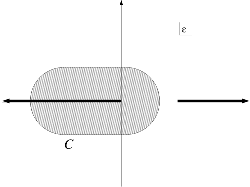
Figure 1: The cuts of $T_{fi}$ in the complex $\varepsilon$ plane. The depicted contour picks up only contributions from the left-hand cut, which corresponds to physical states with a charm quark. The states given by the right-hand cut do not contribute here.

Assuming it is analytic in the shaded region of Fig. 1, the result is

$$\frac{1}{2\pi i}\int_{C}d\varepsilon\,W_{\!\Delta}(\varepsilon)\,T_{fi}(\varepsilon) = \sum_{X_{c}}W_{\!\Delta}(E_{M}\!-\!E_{X_{c}})\frac{\langle\bar{B}(v_{f})|J_{\!f}|X_{c}(v^{\prime})\rangle\langle X_{c}(v^{\prime})|J_{i}|\bar{B}(v_{i})\rangle}{4v^{\prime 0}}\ ,$$ (7)

where the delta function has been used to perform the phase-space integral and the HQET state normalization convention has been used to eliminate mass factors in the denominator. The intermediate $X_{c}$ states carry four-momentum $p_{X_{c}}=m_{X_{c}}v^{\prime}=p_{i}+q$.

Choice of the weight function is governed by well-known concerns bjo ; kap . In practice one uses $W_{\!\Delta}(\varepsilon)=\theta(\Delta+\varepsilon)$, which is the $n\to\infty$ limit of the set of functions

$$W^{(n)}_{\!\Delta}(\varepsilon)=\frac{\Delta^{2n}}{\varepsilon^{2n}+\Delta^{2n}}$$ (8)

for $\varepsilon<0$. But since the weight function must be analytic within the contour, the use of these is strictly correct only for small $n>1$. In this case the poles at $\varepsilon=\sqrt[2n]{-1}\,\Delta$ are a distance of order $\Delta$ away from the cut, and the contour can be deformed away without getting too close to the cut and relying on local duality at a scale below $m_{b}$. This is not true of the $n\to\infty$ limit, in which the poles approach the cut and the contour must pinch the cut at the scale $\Delta$ instead of $m_{b}$. This is a problem because the contribution at $\Delta$ is weighted much more heavily than that at $m_{b}$, and thus the results will depend more strongly on the assumption of local duality. However, an explicit calculation shows that the results here do not depend on $n$, just as the authors of Ref. bjo found in their derivation of corrections to the Bjorken sum rule. This is not true in other cases, such as the Voloshin sum rule bjo . The weight function in what follows can therefore be considered a simple step function excluding states with excitation energies greater than $\Delta$. Although increasing $\Delta$ includes more states and weakens the bounds, the cutoff energy must be chosen large enough to make perturbative QCD appropriate. Choosing $\Delta\gtrsim 2$ GeV should therefore be sufficient.

The sum rule is derived by performing an operator product expansion on the time-ordered product of currents on the left-hand side of Eq. (7) while writing out the right-hand side explicitly in terms of excited-state Isgur-Wise functions. The leading-order OPE relevant for $B$ matrix elements consists of a single dimension-three operator, $\bar{b}_{v_{f}}\Gamma_{\!\!f}(1+{/\hskip-5.29999ptv}\,^{\prime})\Gamma_{\!i}b_{v_{i}}$. Higher dimension operators will be neglected here, as they give corrections suppressed by powers of $\Lambda_{\mathrm{QCD}}/\Delta$ or $\Lambda_{\mathrm{QCD}}/m_{c,b}$. The order $\alpha_{s}$ corrections to the Wilson coefficient of the leading operator are given by a matching calculation involving the diagrams in Figs. 2 and 3.

Figure 2: Diagrams contributing to the order $\alpha_{s}$ corrections to the sum rules. The squares indicate insertions of the currents $J_{i}$ and $J_{\!f}$, respectively. The current $J_{i}$ inserts momentum $q$, while the current $J_{\!f}$ carries away momentum $q^{\prime}$ sufficient to leave the final $b$-quark with velocity $v_{f}$. The velocity-labeled quark fields are those of the heavy quark effective theory.

The generic sum rule resulting from this is

$$\frac{1}{4}\xi(w_{if})[1+\alpha_{s}F(w_{i},w_{f},w_{if})]\,\mathrm{Tr}\left[(1+{/\hskip-5.29999ptv}_{\!f})\,\Gamma_{\!\!f}(1+{/\hskip-5.29999ptv}\,^{\prime})\,\Gamma_{\!i}(1+{/\hskip-5.29999ptv}_{i})\right]$$ (9)

$$=\sum_{X_{c}}W_{\!\Delta}(E_{M}\!-\!E_{X_{c}})\langle\bar{B}(v_{f})|J_{\!f}|X_{c}(v^{\prime})\rangle\langle X_{c}(v^{\prime})|J_{i}|\bar{B}(v_{i})\rangle\ ,$$

where the function $F$ contains the one-loop corrections. In principle, $F$ could be defined to include perturbative corrections of all orders. The form of the corrected sum rule would be the same since HQET vertices are spin independent. The right-hand side is written out explicitly in the next section.

Working in the rest frame of the intermediate hadrons (i.e., $v^{\prime 0}=1$) and using the $\overline{\mathrm{MS}}$ scheme with dimensional regularization and a finite gluon mass $m$, the contributions to $\alpha_{s}F$ of the graphs in Figs. 2(a)–2(d) are, respectively,

$$\frac{2\alpha_{s}}{3\pi}\left(2-\mathrm{ln}\frac{4\Delta^{2}}{\mu^{2}}\right)\ ,$$ (10)

$$\frac{2\alpha_{s}}{3\pi}w_{i}\left\{\frac{\mathrm{ln}\left(w_{i}+\sqrt{w_{i}^{2}-1}\right)}{\sqrt{w_{i}^{2}-1}}\,\mathrm{ln}\frac{4\Delta^{2}}{\mu^{2}}+\int_{0}^{1}dx\,\frac{2\,\mathrm{ln}x-\mathrm{ln}[1+2x(1-x)(w_{i}-1)]}{1+2x(1-x)(w_{i}-1)}\right\}\ ,$$ (11)

$$\frac{2\alpha_{s}}{3\pi}w_{f}\left\{\frac{\mathrm{ln}\left(w_{f}+\sqrt{w_{f}^{2}-1}\right)}{\sqrt{w_{f}^{2}-1}}\,\mathrm{ln}\frac{4\Delta^{2}}{\mu^{2}}+\int_{0}^{1}dx\,\frac{2\,\mathrm{ln}x-\mathrm{ln}[1+2x(1-x)(w_{f}-1)]}{1+2x(1-x)(w_{f}-1)}\right\}\ ,$$ (12)

$$-\frac{4\alpha_{s}}{3\pi}w_{if}\int_{0}^{1}dx\,dy\,dz\,\delta(x+y+z-1)\frac{\theta(z-\sqrt{a}m/\Delta)}{a\sqrt{z^{2}-am^{2}/\Delta^{2}}}\ ,$$ (13)

where $a=1+2xy(w_{if}-1)+2xz(w_{i}-1)+2yz(w_{f}-1)$, and $\alpha_{s}$ is evaluated at subtraction point $\mu$. The contribution of Fig. 2(d) cannot easily be simplified further, but this is no limitation since the sum rules require only the first few terms of $F$ in an expansion about $w_{x}=1$. The graph in Fig. 3 contributes with a minus sign to the matching calculation for the Wilson coefficient, since it gives the renormalization of the leading operator in the OPE, and so its contribution to $\alpha_{s}F$ is

$$\frac{2\alpha_{s}}{3\pi}\frac{w_{if}}{\sqrt{w_{if}^{2}-1}}\,\mathrm{ln}\left(w_{if}+\sqrt{w_{if}^{2}-1}\right)\mathrm{ln}\frac{\mu^{2}}{m^{2}}\ .$$ (14)

This infrared divergence cancels that of the graph in Fig. 2(d), leaving $\alpha_{s}F$ independent of the regulating gluon mass.

Figure 3: One-loop renormalization of the leading operator in the operator product expansion of $T_{fi}$. The blob indicates an insertion of this operator, $\bar{b}_{v_{f}}\Gamma_{\!\!f}(1+{/\hskip-4.76999ptv}\,^{\prime})\Gamma_{\!i}b_{v_{i}}$. The external lines are bottom quarks in the heavy quark effective theory.

From the results above, it is not hard to show that $F(1,w,w)=F(w,1,w)=0$. This important characteristic of the perturbative corrections is true to all orders in $\alpha_{s}$, as can easily be seen. In the limits $v_{i}=v^{\prime}$ and $v_{f}=v^{\prime}$, one of the currents in the time-ordered product is a conserved current associated with heavy quark flavor symmetry and its matrix elements receive no perturbative corrections. Because HQET loop graphs do not change the matrix structures of inserted operators, perturbative corrections to matrix elements of the other current cancel those of the leading operator in the OPE. Therefore, the function analogous to $F$ including perturbative corrections of all orders will still vanish in these limits.

The sum rules derived here are primarily of interest near zero recoil, making it convenient to expand $F$ about $w_{x}=1$ with the definitions

$$\alpha_{s}F(w_{i},w_{f},w_{if}) = b_{if1}(w_{if}-1)+b_{i1}(w_{i}-1)+b_{f1}(w_{f}-1)+\frac{1}{2}b_{if2}(w_{if}-1)^{2}$$ (15)

$$\mbox{}+\frac{1}{2}b_{i2}(w_{i}-1)^{2}+\frac{1}{2}b_{f2}(w_{f}-1)^{2}+b_{i2f}(w_{i}-1)(w_{f}-1)$$

$$\mbox{}+b_{i2if}(w_{i}-1)(w_{if}-1)+b_{f2if}(w_{f}-1)(w_{if}-1)+\cdots\ .$$

There is no zeroth-order term since $F(1,1,1)=0$. This follows from the identities $F(1,w,w)=F(w,1,w)=0$, which also imply

$$b_{f1}+b_{if1}=b_{i1}+b_{if1}=0\ ,$$ (16)

$$b_{f2}+2b_{f2if}+b_{if2}=b_{i2}+2b_{i2if}+b_{if2}=0\ .$$ (17)

These relations between derivatives of the perturbative corrections can be checked at order $\alpha_{s}$ with the explicit values

$$b_{if1}=-b_{f1}=-b_{i1} = \frac{4\alpha_{s}}{9\pi}\left(\frac{5}{3}-\mathrm{ln}\frac{4\Delta^{2}}{\mu^{2}}\right)\ ,$$

$$b_{i2}=b_{f2} = \frac{4\alpha_{s}}{15\pi}\left(\frac{2}{5}-\mathrm{ln}\frac{4\Delta^{2}}{\mu^{2}}\right)\ ,$$

$$b_{if2} = \frac{4\alpha_{s}}{15\pi}\left(-\frac{12}{5}+\mathrm{ln}\frac{4\Delta^{2}}{\mu^{2}}\right)\ ,$$

$$b_{i2if}=b_{f2if} = \frac{4\alpha_{s}}{15\pi}\ ,$$

$$b_{i2f} = -\frac{4\alpha_{s}}{45\pi}\ .$$ (18)

The derivatives above are all specific to the rest frame of intermediate hadrons. This is the frame used henceforth. In other frames (e.g., $v_{i}^{0}=1$) the weight function depends on the $w_{x}$ parameters, and the sum rules are more complicated but not qualitatively different.

III Vector and Axial Vector Sum Rules

When specific matrices $\Gamma_{\!i,f}$ are chosen, the generic sum rule in Eq. (9) can be written out explicitly in terms of excited-state Isgur-Wise functions using Falk’s description of HQET states of arbitrary spin falk . The choice $\Gamma_{\!i,f}={/\hskip-5.29999ptv}_{i,f}$ yields ley2

$$\xi(w_{if})\left[1+\alpha_{s}F(w_{i},w_{f},w_{if})\right](1+w_{i}+w_{f}+w_{if})$$ (19)

$$= (w_{i}+1)(w_{f}+1)\!\sum_{\ell=0}\frac{\ell+1}{2\ell+1}S_{\ell}(w_{i},w_{f},w_{if})\!\sum_{n}\tau_{\ell+1/2}^{(\ell)(n)}(w_{i})\tau_{\ell+1/2}^{(\ell)(n)}(w_{f})W_{\!\Delta}(m_{M}\!-\!m_{\ell+1/2}^{(\ell)(n)})$$

$$\mbox{}+\sum_{\ell=1}S_{\ell}(w_{i},w_{f},w_{if})\!\sum_{n}\tau_{\ell-1/2}^{(\ell)(n)}(w_{i})\tau_{\ell-1/2}^{(\ell)(n)}(w_{f})W_{\!\Delta}(m_{M}\!-\!m_{\ell-1/2}^{(\ell)(n)})\ ,$$

where the weight function now bounds excitation mass because $v^{\prime 0}=1$. The functions $\tau_{\ell\pm 1/2}^{(\ell)(n)}(w)$ are $\bar{B}\to D^{(\ell)(n)}_{\ell\pm 1/2}\,$ Isgur-Wise functions, where $\ell\pm 1/2$ is the spin of the light degrees of freedom, $(-1)^{\ell+1}$ is the parity of the state, and the label $n$ counts “radial excitations.” This name is inspired by the nonrelativistic constituent quark model, but these states can be anything carrying the other quantum numbers, including continuum contributions, for which $n$ would be a continuous parameter and the sums integrals. In that case, the functions $\tau_{\ell\pm 1/2}^{(\ell)(n)}(w)$ would not be Isgur-Wise functions but other $B$ decay form factors. This possibility will be downplayed here, with the assumption that such contributions are small in the bounds derived here. Experimental input on $B\to D\pi l\bar{\nu}$, for example, is needed to evaluate this assumption.

The quark model also offers an interpretation of $\ell$ as the orbital angular momentum between the light antiquark and the heavy quark. The relation of this notation to that of Isgur and Wise iwex for the lower values of $\ell$ is given by

$$\begin{array}[]{r @{,} c @{,} l}\tau_{1/2}^{(0)(n)}(w)=\xi^{(n)}(w)&\quad\tau_{1/2}^{(1)(n)}(w)=2\,\tau_{1/2}^{(n)}(w)&\quad\tau_{3/2}^{(1)(n)}(w)=\sqrt{3}\,\tau_{3/2}^{(n)}(w)\ .\end{array}$$ (20)

The function $S_{\ell}$ takes into account the polarization of an intermediate state with integral spin $\ell$ and is defined as

$$S_{\ell}=v_{i\nu_{1}}\!\!\cdots v_{i\nu_{\ell}}v_{f\mu_{1}}\!\!\cdots v_{f\mu_{\ell}}\sum_{\lambda}\varepsilon_{(\lambda)}^{*\nu_{1}\cdots\nu_{\ell}}\varepsilon_{(\lambda)}^{\mu_{1}\cdots\mu_{\ell}}\ ,$$ (21)

where $\varepsilon^{\mu_{1}\cdots\mu_{\ell}}$ is the polarization tensor of the intermediate state. The sum runs over the $2\ell+1$ polarizations. This quantity was reduced in Ref. ley1 to the relatively simple form

$$S_{\ell}(w_{i},w_{f},w_{if})=\sum_{k=0}^{\ell/2}C_{\ell,k}(w_{i}^{2}-1)^{k}(w_{f}^{2}-1)^{k}(w_{i}w_{f}-w_{if})^{\ell-2k}\,,$$ (22)

with the coefficient

$$C_{\ell,k}=(-1)^{k}\frac{(\ell!)^{2}}{(2\ell)!}\frac{(2\ell-2k)!}{k!(\ell-k)!(\ell-2k)!}\ .$$ (23)

Using this formula it is easy to show that Eq. (19) reduces to

$$2(1+w)\xi(w)[1+\alpha_{s}F(1,w,w)]=2(1+w)\xi(w)$$ (24)

in the limit $v_{i}=v^{\prime}$, confirming that $F(1,w,w)=0$ to all orders. The limit $v_{f}=v^{\prime}$ gives $F(w,1,w)=0$.

The axial sum rule (i.e., Eq. (9) with $\Gamma_{\!i,f}={/\hskip-5.29999ptv}_{i,f}\gamma_{5}$) can be written out explicitly in the same way ley2 :

$$\xi(w_{if})\left[1+\alpha_{s}F(w_{i},w_{f},w_{if})\right](-1+w_{i}+w_{f}-w_{if})$$ (25)

$$= (w_{i}-1)(w_{f}-1)\!\sum_{\ell=1}\frac{\ell}{2\ell-1}S_{\ell-1}(w_{i},w_{f},w_{if})\!\sum_{n}\tau_{\ell-1/2}^{(\ell)(n)}(w_{i})\tau_{\ell-1/2}^{(\ell)(n)}(w_{f})W_{\!\Delta}(m_{M}\!-\!m_{\ell-1/2}^{(\ell)(n)})$$

$$\mbox{}+\sum_{\ell=0}S_{\ell+1}(w_{i},w_{f},w_{if})\!\sum_{n}\tau_{\ell+1/2}^{(\ell)(n)}(w_{i})\tau_{\ell+1/2}^{(\ell)(n)}(w_{f})W_{\!\Delta}(m_{M}\!-\!m_{\ell+1/2}^{(\ell)(n)})\ .$$

As in the vector sum rule, the masses of the intermediate states are denoted by $m_{\ell\pm 1/2}^{(\ell)(n)}$. The limits $v_{i}=v^{\prime}$ and $v_{f}=v^{\prime}$ are trivial for the axial sum rule.

The doublets with spin of the light degrees of freedom $s_{l}=\ell+1/2$ and $s_{l}=\ell-1/2$ contain states with angular momentum $\ell,\,\ell+1$ and $\ell-1,\,\ell$, respectively. But only one member of each doublet contributes to the sum rules in Eqs. (19) and (25) because of the choice of currents. This explains the appearance of only one polarization function for each doublet in the vector and axial vector sum rules.

The zero-recoil normalization of the $\bar{B}\to D^{(*)}$ Isgur-Wise function allows one to write

$$\xi(w)=1-\rho^{2}(w-1)+\frac{\sigma^{2}}{2}(w-1)^{2}-\cdots\ .$$ (26)

The axial and vector sum rules (i.e., Eqs. (19) and (25)) give expressions for $\rho^{2}$, $\sigma^{2}$, and higher derivatives of $\xi(w)$ when differentiated with respect to the parameters $w_{x}$ at $w_{x}=1$. Different combinations of derivatives yield different relations. In the $v^{\prime 0}=1$ frame, the sum rules are invariant under the interchange of $w_{i}$ and $w_{f}$, and it is therefore sufficiently general to consider only derivatives with respect to $w_{if}$ and $w=w_{i}=w_{f}$. Because of this simplification, this paper only uses derivatives of the vector and axial sum rules of the sort

$$\left.\frac{\partial^{p+q}}{\partial w_{if}^{p}\partial w^{q}}\,\right|_{w_{if}=w=1}\ .$$ (27)

Derivatives of the vector sum rule with $p+q=2$ give expressions for $\sigma^{2}$, while the extra factors of $(w_{x}-1)$ in the axial rule require $p+q=3$ for curvature relations.

As an illustration of the method, one can easily derive the Bjorken bjorken ; iwex and Uraltsev uraltsev sum rules with order $\alpha_{s}$ corrections. For this it is only necessary to consider $p+q=1$ in the vector rule and $p+q=2$ in the axial rule. Taking the vector sum rule first, the equation given by the $p=0,\,q=1$ derivative is trivial, but $p=1,\,q=0$ gives the Bjorken sum rule with one-loop corrections bjo :

$$\rho^{2}(\mu)=\frac{1}{4}+\frac{4\alpha_{s}}{9\pi}\left(\frac{5}{3}-\mathrm{ln}\frac{4\Delta^{2}}{\mu^{2}}\right)+2\sum_{n}^{\Delta}\left[\tau_{3/2}^{(n)}(1)\right]^{2}+\sum_{n}^{\Delta}\left[\tau_{1/2}^{(n)}(1)\right]^{2}\ .$$ (28)

This equation has been written in the familiar notation of Isgur and Wise using Eq. (20). The upper limit $\Delta$ on the sums stands for a factor of the weight function $W_{\!\Delta}(m_{M}\!-\!m_{X_{c}})$, which serves to cut off the sums. Without it the results are divergent, as can be seen by attempting to take the $\Delta\to\infty$ limit in the order $\alpha_{s}$ corrections. Note that he subtraction-point dependence is the same on both sides of the equation, since Isgur-Wise functions are independent of $\mu$ at zero recoil while their slopes depend on it logarithmically neubert . This equation should be evaluated near $\mu=\Delta$ to avoid large logarithms in the perturbative expansion.

The lower bound resulting from ignoring the sums in Eq. (28) is similar to one derived in Ref. competbd but somewhat weaker. As discussed in Ref. bjo , this is the result of using different weight functions. That of Ref. competbd is effectively given by the phase space of $b$ decay and falls off faster with $\varepsilon$, thus reducing the contribution of the intermediate states to the sum rule and strengthening the resultant lower bound. A similar effect could be achieved here by using a smaller value for $\Delta$, but as discussed above this makes the use of perturbative QCD less reliable.

The $p=0,\,q=2$ derivative of the axial equation also gives the Bjorken sum rule. The $p=2,\,q=0$ and $p=1,\,q=1$ derivatives give the same result, which, when combined with the Bjorken rule, gives the traditional form of the Uraltsev sum rule:

$$\sum_{n}^{\Delta}\left[\tau_{3/2}^{(n)}(1)\right]^{2}-\sum_{n}^{\Delta}\left[\tau_{1/2}^{(n)}(1)\right]^{2}=\frac{1}{4}-b_{if1}-\frac{1}{2}(b_{i1}+b_{f1})=\frac{1}{4}\ ,$$ (29)

where Eq. (20) has again been used. This equation receives no unsuppressed perturbative corrections. (There are in fact perturbative corrections suppressed by $\Lambda_{\mathrm{QCD}}^{2}/\Delta^{2}$ uraltsev , but such corrections are being neglected here.) In this particular derivation of the Uraltsev rule, this is the result of the relation in Eq. (16) between the first derivatives of $F$. But another derivation from different derivatives of the axial and vector sum rules gives $\alpha_{s}$ corrections proportional to $F(1,1,1)=0$. It appears that the Uraltsev rule is always protected from perturbative corrections by the general identities $F(1,w,w)=F(w,1,w)=0$. This convergent sum rule indicates that $\tau_{1/2}^{(n)}(1)$ and $\tau_{3/2}^{(n)}(1)$ become equal as $n\to\infty$.

Combined with Eq. (28), the Uraltsev rule improves the Bjorken bound significantly:

$$\rho^{2}(\mu)=\frac{3}{4}+b_{if1}(\mu)+3\sum_{n}^{\Delta}\left[\tau_{1/2}^{(n)}(1)\right]^{2}>\frac{3}{4}+\frac{4\alpha_{s}}{9\pi}\left(\frac{5}{3}-\mathrm{ln}\frac{4\Delta^{2}}{\mu^{2}}\right)\ .$$ (30)

Because the Uraltsev rule is not corrected, the corrections to this improved bound are just those of the original Bjorken bound. In particular, they are not substantially increased, as one might expect from the drastic improvement to the bound.

Constraints on the curvature of the Isgur-Wise function are obtained from higher derivatives of the same equations. The three second derivatives of the vector equation and the four third derivatives of the axial can be reduced to five linearly independent relations, as demonstrated in Ref. ley3 . Complete with the one-loop corrections derived here, they are

$$\rho^{2} = -\frac{4}{5}\sum_{n}^{\Delta}\tau_{3/2}^{(1)(n)}(1)\tau_{3/2}^{(1)(n)^{\prime}}(1)+\frac{3}{5}\sum_{n}^{\Delta}\tau_{1/2}^{(1)(n)}(1)\tau_{1/2}^{(1)(n)^{\prime}}(1)+\frac{2}{5}b_{if1}\ ,$$ (31)

$$\sigma^{2} = -\sum_{n}^{\Delta}\tau_{3/2}^{(1)(n)}(1)\tau_{3/2}^{(1)(n)^{\prime}}(1)+b_{if1}\rho^{2}-b_{if2}-\frac{1}{2}\left(b_{i2if}+b_{f2if}\right)\ ,$$ (32)

$$\sigma^{2} = 2\sum_{n}^{\Delta}\left[\tau_{5/2}^{(2)(n)}(1)\right]^{2}+2b_{if1}\rho^{2}-b_{if2}\ ,$$ (33)

$$\sigma^{2} = \frac{5}{4}\rho^{2}+\frac{5}{4}\sum_{n}^{\Delta}\left[\tau_{3/2}^{(2)(n)}(1)\right]^{2}+2b_{if1}\rho^{2}-b_{if2}-\frac{5}{4}b_{if1}\ ,$$ (34)

$$\sigma^{2} = \frac{4}{5}\rho^{2}+\frac{3}{5}\sum_{n}^{\Delta}\left[\tau_{1/2}^{(0)(n)^{\prime}}(1)\right]^{2}+\frac{4}{5}b_{if1}\rho^{2}-\frac{4}{5}b_{if1}-\frac{6}{5}\left(b_{i2if}+b_{f2if}\right)$$ (35)

$$\mbox{}-\frac{8}{5}b_{if2}-\frac{3}{10}\left(b_{i2}+2b_{i2f}+b_{f2}\right)\ .$$

The last two equations give the bounds of Ref. ley3 , complete with order $\alpha_{s}$ corrections. Only a couple of orbital excitations occur and in positive-definite form, allowing the derivation of nontrivial lower bounds. Using the values of Eqs. (II) gives

$$\sigma^{2}(\mu) > \frac{5}{4}\rho^{2}(\mu)\left(1+\frac{32\alpha_{s}}{27\pi}-\frac{32\alpha_{s}}{45\pi}\,\mathrm{ln}\frac{4\Delta^{2}}{\mu^{2}}\right)-\frac{193\alpha_{s}}{675\pi}+\frac{13\alpha_{s}}{45\pi}\,\mathrm{ln}\frac{4\Delta^{2}}{\mu^{2}}\ ,$$ (36)

$$\sigma^{2}(\mu) > \frac{3}{5}\left[\rho^{2}(\mu)\right]^{2}+\frac{4}{5}\rho^{2}(\mu)\left(1+\frac{20\alpha_{s}}{27\pi}-\frac{4\alpha_{s}}{9\pi}\,\mathrm{ln}\frac{4\Delta^{2}}{\mu^{2}}\right)-\frac{148\alpha_{s}}{675\pi}+\frac{4\alpha_{s}}{45\pi}\,\mathrm{ln}\frac{4\Delta^{2}}{\mu^{2}}\ ,$$ (37)

where the identity $\tau_{1/2}^{(0)(0)^{\prime}}(1)=-\rho^{2}$ has been used. As demonstrated below in the derivation of physical bounds, the subtraction-point dependence is the same on both sides of these inequalities.

IV Physical Bounds

When combined with $\alpha_{s}$ and $\Lambda_{\mathrm{QCD}}/m_{c,b}$ corrections from matching HQET onto the full theory, the curvature bounds derived above imply bounds on the zero-recoil derivatives of the functions $\mathcal{F}_{D^{(*)}}(w)$. It is convenient to expand these functions about the zero-recoil point according to

$$\mathcal{F}_{D^{(*)}}(w)=\mathcal{F}_{D^{(*)}}(1)\left[1-\rho^{2}_{D^{(*)}}(w-1)+\frac{\sigma^{2}_{D^{(*)}}}{2}(w-1)^{2}-\cdots\right]\ .$$ (38)

A simple matching calculation, taken from Ref. neubert , yields the relations between the Isgur-Wise derivatives and those of the physical shape functions:

$$\rho_{D^{(*)}}^{2} = \rho^{2}(\mu)+\frac{4\alpha_{s}}{9\pi}\,\mathrm{ln}\frac{m_{c}^{2}}{\mu^{2}}+\frac{\alpha_{s}}{\pi}\left(\delta_{D^{(*)}}^{(\alpha_{s})}-\frac{20}{27}\right)+\frac{\bar{\Lambda}}{2m_{c}}\delta_{D^{(*)}}^{(1/m)}\ ,$$

$$\sigma_{D^{(*)}}^{2} = \sigma^{2}(\mu)+2\rho^{2}(\mu)\left[\frac{4\alpha_{s}}{9\pi}\,\mathrm{ln}\frac{m_{c}^{2}}{\mu^{2}}+\frac{\alpha_{s}}{\pi}\left(\delta_{D^{(*)}}^{(\alpha_{s})}-\frac{20}{27}\right)\right]+\frac{4\alpha_{s}}{15\pi}\,\mathrm{ln}\frac{m_{c}^{2}}{\mu^{2}}$$ (39)

$$\mbox{}+\frac{\alpha_{s}}{\pi}\left(\Delta_{D^{(*)}}^{(\alpha_{s})}-\frac{16}{25}\right)+\frac{\bar{\Lambda}}{2m_{c}}\Delta_{D^{(*)}}^{(1/m)}\ .$$

The perturbative corrections are model independent. The parameters $\delta_{D^{(*)}}^{(\alpha_{s})}$ and $\Delta_{D^{(*)}}^{(\alpha_{s})}$ are given by

$$\delta_{D^{*}}^{(\alpha_{s})} = \frac{2(1-z)(11+2z+11z^{2})+24(2-z+z^{2})z\,\mathrm{ln}z}{27(1-z)^{3}}=0.24\ ,$$

$$\delta_{D}^{(\alpha_{s})} = \frac{2(1-z)(23-34z+23z^{2})+12(3-3z+2z^{2})z\,\mathrm{ln}z}{27(1-z)^{3}}=1.20\ ,$$

$$\Delta_{D^{*}}^{(\alpha_{s})} = -\frac{8(47+17z+252z^{2}+17z^{3}+47z^{4})}{675(1-z)^{4}}$$

$$\mbox{}-\frac{4(5+125z-55z^{2}+95z^{3}-18z^{4})z\,\mathrm{ln}z}{135(1-z)^{5}}=-1.16\ ,$$

$$\Delta_{D}^{(\alpha_{s})} = \frac{4(47-258z+302z^{2}-258z^{3}+47z^{4})}{225(1-z)^{4}}$$ (40)

$$\mbox{}-\frac{8(5-5z+5z^{2}-z^{3})z^{2}\,\mathrm{ln}z}{15(1-z)^{5}}=0.63\ ,$$

where $z=m_{c}/m_{b}$, and the approximation $r_{(*)}\approx z$ has been made in the order $\alpha_{s}$ corrections. These values agree with those calculated in Ref. grinlig . The numerical values are for $m_{c}=1.4$ GeV and $m_{b}=4.8$ GeV.

The nonperturbative corrections cannot currently be calculated model-independently because they depend on the four subleading Isgur-Wise functions that parameterize first-order corrections to the heavy-quark limit, $\chi_{1-3}(w)$ and $\eta(w)$. But they can be estimated using QCD sum rules qcdsum (and, in principle, lattice QCD). In the notation of Neubert neubert , the nonperturbative corrections are

$$\delta_{D^{*}}^{(1/m)} = -2\chi_{1}^{\prime}(1)(1+z)-\frac{4}{3}\chi_{2}(1)(1-3z)+4\chi_{3}^{\prime}(1)(1-3z)$$

$$\mbox{}-\frac{5}{6}(1+z)-\frac{1-2z+5z^{2}}{3(1-z)}\eta(1)\approx-2.1\ ,$$

$$\delta_{D}^{(1/m)} = -2(1+z)\left[\chi_{1}^{\prime}(1)-2\chi_{2}(1)+6\chi_{3}^{\prime}(1)\right]+\frac{2(1-z)^{2}}{1+z}\eta^{\prime}(1)\approx-1.3\ ,$$

$$\Delta_{D^{*}}^{(1/m)} = \rho^{2}\left[-2\eta(1)\frac{1-2z+5z^{2}}{3(1-z)}-\frac{5}{3}(1+z)\right]+2(1+z)\chi_{1}^{\prime\prime}(1)-\frac{8(1-6z+z^{2})\chi_{2}(1)}{9(1-z)^{2}}$$

$$\mbox{}+\frac{8}{3}(1-3z)\chi_{2}^{\prime}(1)-4(1-3z)\chi_{3}^{\prime\prime}(1)-\frac{\eta(1)(5-28z+18z^{2}-52z^{3}+25z^{4})}{9(1-z)^{3}}$$

$$\mbox{}+\frac{2\eta^{\prime}(1)(1-2z+5z^{2})}{3(1-z)}-\frac{(1+z)(25-42z+25z^{2})}{18(1-z)^{2}}\approx-2.6\rho^{2}-1.7\ ,$$

$$\Delta_{D}^{(1/m)} = 4\rho^{2}\eta^{\prime}(1)\frac{(1-z)^{2}}{1+z}+2(1+z)\left[\chi_{1}^{\prime\prime}(1)-4\chi_{2}^{\prime}(1)+6\chi_{3}^{\prime\prime}(1)\right]-2\eta^{\prime\prime}(1)\frac{(1-z)^{2}}{1+z}$$ (41)

$$\approx -0.3\ ,$$

where the primes denote $d/dw$. In these corrections $\rho^{2}$ can be taken to be $\rho_{D^{(*)}}^{2}$, since the results here do not include corrections of order $\alpha_{s}\Lambda_{\mathrm{QCD}}/m_{c,b}$. The parts of these expressions for $\Delta_{D^{*}}^{(1/m)}$ and $\Delta_{D}^{(1/m)}$ proportional to $\rho^{2}$ disagree with those of Ref. grinlig . The numerical estimates are based on the approximate values $\eta(1)=0.6$, $\eta^{\prime}(1)=0$, $\chi_{1}^{\prime}(1)=0.3$, $\chi_{2}(1)=-0.04$, $\chi_{2}^{\prime}(1)=0.03$, and $\chi_{3}^{\prime}(1)=0.02$ qcdsum . The values $\eta^{\prime\prime}(1)=\chi_{1}^{\prime\prime}(1)=\chi_{3}^{\prime\prime}(1)=0$ and $z=0.29$ were also used. Since these values are model dependent with large uncertainties, the numerical estimates of the nonperturbative corrections should be interpreted with caution. Reliable lattice results would be a welcome check on such large QCD sum rule estimates of these corrections.

Combining the bounds of Eqs. (36) and (37) with Eqs. (IV) gives the physical bounds

$$\sigma_{D^{(*)}}^{2} > \frac{5}{4}\rho_{D^{(*)}}^{2}\left(1+\frac{8\alpha_{s}}{5\pi}\delta_{D^{(*)}}^{(\alpha_{s})}+\frac{32\alpha_{s}}{45\pi}\,\mathrm{ln}\frac{m_{c}^{2}}{4\Delta^{2}}\right)-\frac{13\alpha_{s}}{45\pi}\,\mathrm{ln}\frac{m_{c}^{2}}{4\Delta^{2}}-\frac{5\alpha_{s}}{4\pi}\delta_{D^{(*)}}^{(\alpha_{s})}+\frac{\alpha_{s}}{\pi}\Delta_{D^{(*)}}^{(\alpha_{s})}$$ (42)

$$\mbox{}-\frac{5}{4}\frac{\bar{\Lambda}}{2m_{c}}\delta_{D^{(*)}}^{(1/m)}+\frac{\bar{\Lambda}}{2m_{c}}\Delta_{D^{(*)}}^{(1/m)}\ ,$$

$$\sigma_{D^{(*)}}^{2} > \frac{3}{5}\left(\rho_{D^{(*)}}^{2}\right)^{2}+\frac{4}{5}\rho_{D^{(*)}}^{2}\left(1+\frac{4\alpha_{s}}{9\pi}\,\mathrm{ln}\frac{m_{c}^{2}}{4\Delta^{2}}+\frac{\alpha_{s}}{\pi}\delta_{D^{(*)}}^{(\alpha_{s})}-\frac{3}{2}\frac{\bar{\Lambda}}{2m_{c}}\delta_{D^{(*)}}^{(1/m)}\right)-\frac{4\alpha_{s}}{45\pi}\,\mathrm{ln}\frac{m_{c}^{2}}{4\Delta^{2}}$$ (43)

$$\mbox{}-\frac{4\alpha_{s}}{15\pi}-\frac{4\alpha_{s}}{5\pi}\delta_{D^{(*)}}^{(\alpha_{s})}+\frac{\alpha_{s}}{\pi}\Delta_{D^{(*)}}^{(\alpha_{s})}-\frac{4}{5}\frac{\bar{\Lambda}}{2m_{c}}\delta_{D^{(*)}}^{(1/m)}+\frac{\bar{\Lambda}}{2m_{c}}\Delta_{D^{(*)}}^{(1/m)}\ .$$

Numerically, these inequalities are

$$\sigma_{D^{*}}^{2} > \frac{5}{4}\rho_{D^{*}}^{2}[1-0.11(0.16)_{p}-0.3_{np}]-0.081(0.059)_{p}+0.1_{np}\ ,$$

$$\sigma_{D^{*}}^{2} > \frac{3}{5}\left(\rho_{D^{*}}^{2}\right)^{2}+\frac{4}{5}\rho_{D^{*}}^{2}[1-0.066(0.101)_{p}+0.08_{np}]-0.14(0.13)_{p}-0.003_{np}\ ,$$

$$\sigma_{D}^{2} > \frac{5}{4}\rho_{D}^{2}[1+0.041(-0.014)_{p}+0.0_{np}]-0.025(0.0028)_{p}+0.2_{np}\ ,$$

$$\sigma_{D}^{2} > \frac{3}{5}\left(\rho_{D}^{2}\right)^{2}+\frac{4}{5}\rho_{D}^{2}[1+0.025(-0.0089)_{p}+0.3_{np}]-0.039(0.032)_{p}+0.1_{np}\ ,$$ (44)

where the values $\alpha_{s}=0.3$ (in the $\overline{\mathrm{MS}}$ scheme around 2 GeV) and $\bar{\Lambda}=0.4$ GeV have been used. The perturbative corrections, with subscript $p$, are for two values of $\Delta$. The results for $\Delta=2$ GeV are first, and those for $\Delta=3$ GeV are in parentheses. The nonperturbative corrections are labeled by a subscript $np$.

Equations (42) and (43) imply absolute bounds when combined with the corrected form of the Uraltsev bound,

$$\rho_{D^{(*)}}^{2}>\frac{3}{4}+\frac{4\alpha_{s}}{9\pi}\,\mathrm{ln}\frac{m_{c}^{2}}{4\Delta^{2}}+\frac{\alpha_{s}}{\pi}\delta_{D^{(*)}}^{(\alpha_{s})}+\frac{\bar{\Lambda}}{2m_{c}}\delta_{D^{(*)}}^{(1/m)}\ ,$$ (45)

which comes from Eq. (30) and the first of Eqs. (IV), and the tree-level Voloshin bound volosh , $\rho^{2}\lesssim 3/4$. A lower bound is required for terms proportional to $\rho_{D^{(*)}}^{2}$ with positive coefficients, and an upper bound is required for those with negative coefficients. The latter are corrections, so the upper bound is only needed at tree level. Note that an upper bound is required to estimate the greatest impact the corrections could have on the bound.

Inserting these inequalities into Eq. (42) gives

$$\sigma_{D^{(*)}}^{2}>\frac{15}{16}+\frac{14\alpha_{s}}{15\pi}\,\mathrm{ln}\frac{m_{c}^{2}}{4\Delta^{2}}+\frac{3\alpha_{s}}{2\pi}\delta_{D^{(*)}}^{(\alpha_{s})}+\frac{\alpha_{s}}{\pi}\Delta_{D^{(*)}}^{(\alpha_{s})}+\frac{\bar{\Lambda}}{2m_{c}}\Delta_{D^{(*)}}^{(1/m)}\ ,$$ (46)

where $\rho_{D^{(*)}}^{2}$ is replaced by $3/4$ in $\Delta_{D^{(*)}}^{(1/m)}$. The absolute bound produced in the same way from Eq. (43) happens to be identical at leading order and weaker only by the addition of $-4\alpha_{s}/15\pi$ after perturbative and $\Lambda_{\mathrm{QCD}}/m_{c,b}$ corrections are included. Using the numerical estimates above, the bounds in Eq. (46) are

$$\sigma_{D^{*}}^{2} > 0.94-0.26(0.34)_{p}-0.5_{np}\ ,$$

$$\sigma_{D}^{2} > 0.94+0.045(-0.027)_{p}-0.04_{np}\ ,$$ (47)

where the corrections are labeled as described above.

When considering the bounds in Eqs. (45) and (46) and their dependence on $\Delta$, one must bear in mind that the logarithms in the perturbative corrections are only small if $\Delta$, $m_{b}$, and $m_{c}$ are roughly of the same order. That is the accuracy of the results obtained here. For instance, Eq. (IV) is valid for $\mu$ on the order of $m_{c,b}$, while Eqs. (36) and (37) are valid for $\mu$ near $\Delta$. Therefore, taking the $\Delta\to\infty$ limit does not make sense in the absolute bounds. To understand the behavior of the bounds in this limit, one would need to sum the logarithms of $m_{c}^{2}/\Delta^{2}$. Since these logarithms are not large for the values of $\Delta$ used here, this extra step has been omitted.

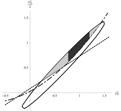
Figure 4: Dispersive constraints on $\mathcal{F}_{D}$ derivatives combined with the corrected sum rule bounds derived here at $\Delta=2$ GeV. The interior of the ellipse is the region allowed by the dispersion relations. Including the curvature bounds, given by the area above the dashed curves, further restricts the allowed region to the shaded area. The darker region is obtained by also including the Bjorken and Voloshin bounds. Both perturbative and nonperturbative corrections are included.

The sum rule bounds derived here should be compared with the dispersive constraints usually used to guide the extrapolation of measured form factors to zero recoil. These constraints are derived by computing the vacuum expectation value of a time-ordered product of $b\to c$ currents in the perturbative regime and then using analyticity to learn about the semileptonic regime. The result is equated with a spectral function sum of resonances (i.e., a sum of positive quantities). Much as in the derivation of the sum rules here, focusing on specific resonances yields form factor constraints. A typical example is shown in Fig. 4. The slope and curvature must lie within the ellipse, a constraint that is well approximated by a linear relation between the slope and curvature. Data are fit as a function of $w$ for $|V_{cb}|\mathcal{F}_{D^{(*)}}(1)$ and $\rho_{D^{(*)}}^{2}$, and the second derivative at zero recoil is related to the slope according to this relation. For the process $\bar{B}^{0}\to D^{+}\ell^{-}\bar{\nu}$, Belle used the relation $\sigma_{D}^{2}/2=1.05\rho_{D}^{2}-0.15$ disper2 to find $\sigma_{D}^{2}=2.06\pm 0.46\pm 0.29$, where the first uncertainty is statistical and the second systematic belle1 . This value is consistent with the bound above.

Rather than $\mathcal{F}_{D^{*}}(w)$, one typically fits the shape of the axial vector form factor $h_{A_{1}}(w)$, which is defined, for example, in Ref. grinlig . Like $\mathcal{F}_{D^{*}}(w)$, it is equal to the Isgur-Wise function $\xi(w)$ in the heavy-quark limit. Its curvature is defined as in Eq. (38) and satisfies the bound in Eq. (46), with perturbative and nonperturbative corrections given by

$$\delta_{A_{1}}^{(\alpha_{s})} = \frac{2(1-z)(17-4z+17z^{2})+6(9-3z+4z^{2})z\,\mathrm{ln}z}{27(1-z)^{3}}=0.65\ ,$$

$$\delta_{A_{1}}^{(1/m)} = -2(1+z)\chi_{1}^{\prime}(1)+4z\chi_{2}(1)+4\chi_{3}^{\prime}(1)(1-3z)+z\eta(1)-\frac{1+z}{2}\approx-1.3\ ,$$

$$\Delta_{A_{1}}^{(\alpha_{s})} = \frac{4(1-z)(27-203z-68z^{2}-203z^{3}+27z^{4})-120(10+5z^{2}-z^{3})z^{2}\,\mathrm{ln}z}{225(1-z)^{5}}=0.24\ ,$$

$$\Delta_{A_{1}}^{(1/m)} = \rho^{2}[2z\eta(1)-1-z]+2\chi_{1}^{\prime\prime}(1)(1+z)-8z\chi_{2}^{\prime}(1)-4\chi_{3}^{\prime\prime}(1)(1-3z)$$ (48)

$$\mbox{}+z\eta(1)-2z\eta^{\prime}(1)-\frac{1+z}{2}\approx-0.9\rho^{2}-0.5\ ,$$

where the numerical estimates are based on the values used above. These values produce the absolute bound

$$\sigma_{A_{1}}^{2}>.94-0.071(0.14)_{p}-0.2_{np}$$ (49)

on the curvature of $h_{A_{1}}(w)$. This should be compared with the value found by Belle by the procedure described above for the process $\bar{B}^{0}\to D^{*+}e^{-}\bar{\nu}$. Using the relation $\sigma_{A_{1}}^{2}/2=1.08\rho_{A_{1}}^{2}-0.23$ disper2 , Belle found $\sigma_{A_{1}}^{2}=2.44\pm 0.37\pm 0.41$, where the first uncertainty is statistical and the second systematic belle2 . This value is also consistent with the bound produced here. A plot comparing dispersive constraints and sum rule bounds for this form factor would be similar to Fig. 4, but with the sum rule bounds comparatively somewhat weaker.

V Conclusions

This paper has presented order $\alpha_{s}$ corrections to two new sum rules derived in Refs. ley1 ; ley2 ; ley3 in the context of HQET. Section II repeated the tree-level derivation of a generic sum rule depending on three velocity transfer variables and included one-loop corrections. Section III studied the axial vector and vector sum rules that result from choosing specific currents in the generic equation. These led to $\alpha_{s}$-corrected versions of the sum rules of Le Yaouanc et al. for the curvature of the Isgur-Wise function. There were no corrections suppressed by the heavy quark masses because the infinite-mass limit was used. Section IV translated these HQET bounds into bounds on physical form factors by including perturbative and finite-mass corrections associated with matching HQET onto the full theory. Numerical estimates were given and compared with experimental values and dispersive constraints. The bounds produced here are less powerful than dispersive constraints but may provide an important check on those constraints.

References

• (1) E. Eichten and B. Hill, Phys. Lett. B 234, 511 (1990); H. Georgi, Phys. Lett. B 240, 447 (1990).
• (2) N. Isgur and M. B. Wise, Phys. Lett. B 232, 113 (1989); Phys. Lett. B 237, 527 (1990).
• (3) S. Nussinov and W. Wetzel, Phys. Rev. D 36, 130 (1987).
• (4) M. A. Shifman and M. B. Voloshin, Sov. J. Nucl. Phys.  47, 511 (1988) [Yad. Fiz.  47, 801 (1988)].
• (5) M. E. Luke, Phys. Lett. B 252, 447 (1990).
• (6) A. Czarnecki, Phys. Rev. Lett.  76, 4124 (1996); A. Czarnecki and K. Melnikov, Nucl. Phys. B 505, 65 (1997).
• (7) S. Stone, in B Decays, 2nd Edition, edited by S. Stone (World Scientific, Singapore 1994), p. 283.
• (8) C. G. Boyd, B. Grinstein and R. F. Lebed, Phys. Lett. B 353, 306 (1995); Nucl. Phys. B 461, 493 (1996); Phys. Rev. D 56, 6895 (1997).
• (9) I. Caprini and M. Neubert, Phys. Lett. B 380, 376 (1996); I. Caprini, L. Lellouch and M. Neubert, Nucl. Phys. B 530, 153 (1998).
• (10) A. Le Yaouanc, L. Oliver and J. C. Raynal, Phys. Rev. D 67, 114009 (2003).
• (11) A. Le Yaouanc, L. Oliver and J. C. Raynal, Phys. Lett. B 557, 207 (2003).
• (12) A. Le Yaouanc, L. Oliver and J. C. Raynal, Phys. Rev. D 69, 094022 (2004).
• (13) I. Bigi, M. Shifman, N. G. Uraltsev and A. Vainshtein, Phys. Rev. D 52, 196 (1995).
• (14) A. Kapustin, Z. Ligeti, M. B. Wise and B. Grinstein, Phys. Lett. B 375, 327 (1996).
• (15) C. G. Boyd and I. Z. Rothstein, Phys. Lett. B 395, 96 (1997).
• (16) C. G. Boyd, Z. Ligeti, I. Z. Rothstein and M. B. Wise, Phys. Rev. D 55, 3027 (1997).
• (17) N. Uraltsev, Phys. Lett. B 501, 86 (2001).
• (18) E. C. Poggio, H. R. Quinn and S. Weinberg, Phys. Rev. D 13, 1958 (1976).
• (19) A. F. Falk, Nucl. Phys. B 378, 79 (1992).
• (20) N. Isgur and M. B. Wise, Phys. Rev. D 43, 819 (1991).
• (21) J. D. Bjorken, SLAC-PUB-5278 Invited talk given at Les Rencontres de la Valle d’Aoste, La Thuile, Italy, Mar 18-24, 1990; J. D. Bjorken, I. Dunietz and J. Taron, Nucl. Phys. B 371, 111 (1992).
• (22) M. Neubert, Phys. Rept.  245, 259 (1994).
• (23) C. G. Boyd, B. Grinstein and A. V. Manohar, Phys. Rev. D 54, 2081 (1996).
• (24) B. Grinstein and Z. Ligeti, Phys. Lett. B 526, 345 (2002).
• (25) M. Neubert, Phys. Rev. D 46, 3914 (1992); M. Neubert, Z. Ligeti and Y. Nir, Phys. Lett. B 301, 101 (1993); Phys. Rev. D 47, 5060 (1993); Z. Ligeti, Y. Nir and M. Neubert, Phys. Rev. D 49, 1302 (1994).
• (26) M. B. Voloshin, Phys. Rev. D 46, 3062 (1992).
• (27) K. Abe et al. [Belle Collaboration], Phys. Lett. B 526, 258 (2002).
• (28) K. Abe et al. [Belle Collaboration], Phys. Lett. B 526, 247 (2002).