Interpreting the time-dependent CP asymmetry in $B^{0}\to\pi^{0}K_{S}$

Michael Gronau^a,b, Yuval Grossman,^a,b,c and Jonathan L. Rosner^d,

^aStanford Linear Accelerator Center,
Stanford University, Stanford, CA 94309
^bDepartment of Physics, Technion – Israel Institute of Technology,
Technion City, 32000 Haifa, Israel
^cSanta Cruz Institute for Particle Physics,
University of California, Santa Cruz, CA 95064
^dLaboratory of Elementary Particle Physics
Cornell University, Ithaca, New York 14850

Flavor SU(3) is used for studying the time-dependent CP asymmetry in $B^{0}\to\pi^{0}K_{S}$ by relating this process to $B^{0}\to\pi^{0}\pi^{0}$ and $B^{0}\to K^{+}K^{-}$. We calculate correlated bounds on $S_{\pi K}-\sin 2\beta$ and $C_{\pi K}$, with maximal magnitudes of 0.2 and 0.3, where $S_{\pi K}$ and $C_{\pi K}$ are coefficients of $\sin\Delta mt$ and $\cos\Delta mt$ in the asymmetry. Stronger upper limits on $B^{0}\to K^{+}K^{-}$ are expected to reduce these bounds and to imply nonzero lower limits on these observables. The asymmetry is studied as a function of a strong phase and the weak phase $\gamma$.

  PACS codes: 12.15.Hh, 12.15.Ji, 13.25.Hw, 14.40.Nd

The time-dependent CP asymmetry measured in $B\to J/\psi K_{S}$ [1] confirmed the Standard Model, verifying that the Kobayashi-Maskawa phase [2] is the dominant origin of CP violation in $K$ and $B$ meson decays. The theoretical interpretation of this measurement in terms of $\sin 2\beta$, where $2\beta\equiv{\rm Arg}(V^{*}_{td})$ is the phase of $B^{0}-\bar{B}^{0}$ mixing [3], is pure because a single weak phase dominates the weak amplitude of $B^{0}\to J/\psi K_{S}$ to a high accuracy [4]. Charmless strangeness changing $B^{0}$ decays into $\phi K_{S},~{}\eta^{\prime}K_{S}$ and $K^{+}K^{-}K_{S}$ measured recently [5] involve contributions with a second weak phase which differs from the phase of the dominant penguin amplitude. This modifies the time-dependent asymmetries of these processes, which involve hadronic uncertainties due to the unknown magnitude and strong phase of the small amplitude relative to the dominant one. Model-independent upper bounds on these effects were studied using SU(3) or U-spin [6, 7, 8, 9, 10]. These bounds may be used to indicate when a deviation from the Standard Model is observed in asymmetry measurements [11].

Recently a first measurement of the CP asymmetry in $B^{0}(t)\to\pi^{0}K_{S}$ was reported [12],

$$S_{\pi K}=0.48^{+0.38}_{-0.47}\pm 0.11~{},~{}~{}~{}~{}C_{\pi K}=0.40^{+0.27}_{-0.28}\pm 0.10~{}~{},$$ (1)

where $S_{\pi K}$ and $-C_{\pi K}$ are coefficients of $\sin\Delta mt$ and $\cos\Delta mt$ terms in the time-dependent asymmetry,

$$A(t)\equiv\frac{\Gamma(\bar{B}^{0}(t)\to\pi^{0}K_{S})-\Gamma(B^{0}(t)\to\pi^{0}K_{S})}{\Gamma(\bar{B}^{0}(t)\to\pi^{0}K_{S})+\Gamma(B^{0}(t)\to\pi^{0}K_{S})}=-C_{\pi K}\cos(\Delta mt)+S_{\pi K}\sin(\Delta mt)~{}.$$ (2)

The currently measured branching ratio for decays into $\pi^{0}K^{0}$, averaged over $B^{0}$ and $\bar{B}^{0}$, is [13]

$$\bar{\cal B}(B^{0}\to\pi^{0}K^{0})=(11.92\pm 1.44)\times 10^{-6}~{}.$$ (3)

In the present Letter we interpret the results for the two asymmetries $S_{\pi K}$ and $C_{\pi K}$ in terms of the two amplitudes contributing to this process and their relative strong and weak phases. The relative weak phase between the two interfering amplitudes is the CKM phase $\gamma\equiv{\rm Arg}(V^{*}_{ub})$. Using flavor SU(3), we find a relation between deviations from $S_{\pi K}=\sin 2\beta$ and $C_{\pi K}=0$ and decay rates for $B^{0}\to\pi^{0}\pi^{0}$ and $B^{0}\to K^{+}K^{-}$. The major purpose of this study is to provide, within the CKM framework, both upper and lower bounds on these deviations in terms of measured rates. It will also be shown how to obtain information about $\gamma$ if such deviations are measured within the range allowed in the Standard Model.

We decompose the amplitude for $B^{0}\to\pi^{0}K^{0}$ into two terms involving CKM factors $V^{*}_{cb}V_{cs}$ and $V^{*}_{ub}V_{us}$, which we denote by $p^{\prime}/\sqrt{2}$ and $-c^{\prime}/\sqrt{2}$, respectively,

$$A(B^{0}\to\pi^{0}K^{0})={p^{\prime}-c^{\prime}\over\sqrt{2}}~{},\qquad p^{\prime}\equiv|p^{\prime}|e^{i\delta}~{},\qquad c^{\prime}\equiv|c^{\prime}|e^{i\gamma}~{}.$$ (4)

This parameterization is true in general within the Standard Model. The two terms, a penguin amplitude $p^{\prime}$ with strong phase $\delta$ and a color-suppressed tree amplitude $c^{\prime}$ with weak phase $\gamma$, are graphical representations of SU(3) amplitudes [14] of which we make use below. The amplitude $p^{\prime}$ contains color-allowed and color-suppressed contributions from electroweak penguin operators, $p^{\prime}\equiv P^{\prime}-P^{\prime}_{\rm EW}-P^{\prime c}_{\rm EW}/3$ [15].

Expressions for $S_{\pi K}$ and $C_{\pi K}$ in terms of $p^{\prime}$ and $c^{\prime}$ can be obtained from definitions, taking into account the negative CP eigenvalue of $\pi^{0}K_{S}$ in $B^{0}$ decays:

$$S_{\pi K}\equiv\frac{2{\rm Im}(\lambda_{\pi K})}{1+|\lambda_{\pi K}|^{2}}~{},~{}~{}~{}~{}~{}~{}~{}~{}~{}C_{\pi K}\equiv\frac{1-|\lambda_{\pi K}|^{2}}{1+|\lambda_{\pi K}|^{2}}~{},$$ (5)

where

$$\lambda_{\pi K}\equiv-e^{-2i\beta}\frac{A(\bar{B}^{0}\to\pi^{0}\bar{K}^{0})}{A(B^{0}\to\pi^{0}K^{0})}~{}.$$ (6)

Using Eq. (4), the asymmetries $S_{\pi K}$ and $C_{\pi K}$ are then written in terms of $|c^{\prime}/p^{\prime}|,~{}\delta$, $\gamma$, and $\alpha\equiv\pi-\beta-\gamma$, as

$$S_{\pi K} = {\sin 2\beta-2|c^{\prime}/p^{\prime}|\cos\delta\sin(2\beta+\gamma)-|c^{\prime}/p^{\prime}|^{2}\sin(2\alpha)\over R_{00}}~{},$$ (7)

$$C_{\pi K} = -{2|c^{\prime}/p^{\prime}|\sin\delta\sin\gamma\over R_{00}}~{},$$ (8)

$$R_{00} \equiv 1-2|c^{\prime}/p^{\prime}|\cos\delta\cos\gamma+|c^{\prime}/p^{\prime}|^{2}~{}.$$ (9)

The amplitudes $p^{\prime}$ and $c^{\prime}$ are expected to obey a hierarchy, $|c^{\prime}|\ll|p^{\prime}|$ [14, 15], which will be justified later on using experimental data. In the limit of neglecting $c^{\prime}$, one has the well-known result $S_{\pi K}=\sin 2\beta,C_{\pi K}=0$. Keeping only linear terms in $|c^{\prime}/p^{\prime}|$, one has [16]

$$\Delta S_{\pi K}\equiv S_{\pi K}-\sin 2\beta\approx-2|c^{\prime}/p^{\prime}|\cos 2\beta\cos\delta\sin\gamma~{},~{}~{}~{}~{}~{}C_{\pi K}\approx-2|c^{\prime}/p^{\prime}|\sin\delta\sin\gamma~{}.$$ (10)

Precise knowledge of the ratio $|c^{\prime}/p^{\prime}|$ would permit a determination of $\sin^{2}\gamma$ from the two measurements of $S_{\pi K}$ and $C_{\pi K}$ [7],

$$\sin^{2}\gamma\approx\frac{1}{4|c^{\prime}/p^{\prime}|^{2}}\left(C^{2}_{\pi K}+(\Delta S_{\pi K}/\cos 2\beta)^{2}\right)~{}.$$ (11)

Our goal is to obtain information about $|c^{\prime}/p^{\prime}|$ from other $B$ decays using flavor SU(3). For this purpose, we write expressions within flavor SU(3) for the amplitudes of two strangeness conserving $B^{0}$ decays [14, 15],

$$A(B^{0}\to\pi^{0}\pi^{0}) = (p-c+e+pa)/\sqrt{2}~{},$$ (12)

$$A(B^{0}\to K^{+}K^{-}) = -(e+pa)~{}~{}.$$ (13)

The amplitudes $p$ and $c$ in $\Delta S=0$ decays, defined in analogy with $p^{\prime}$ and $c^{\prime}$ in $\Delta S=1$ decays, involve CKM factors $V^{*}_{cb}V_{cd}$ and $V^{*}_{ub}V_{ud}$, respectively. The exchange ($e$) and penguin annihilation ($pa$) amplitudes occurring in the second process are expected to be negligible, unless enhanced by rescattering [17]. Current branching ratio measurements, averaged over $B^{0}$ and $\bar{B}^{0}$, are [13]

$$\bar{\cal B}(B^{0}\to\pi^{0}\pi^{0}) = (1.89\pm 0.46)\times 10^{-6}~{},$$ (14)

$$\bar{\cal B}(B^{0}\to K^{+}K^{-}) < 0.6\times 10^{-6}~{}(90\%~{}{\rm confidence~{}level})~{}.$$ (15)

These values already indicate some suppression of $e+pa$ relative to $p-c$. Using the $90\%$ confidence level upper bound on $\bar{\cal B}(B^{0}\to K^{+}K^{-})$ and the central value of $\bar{\cal B}(B^{0}\to\pi^{0}\pi^{0})$ we obtain the $90\%$ confidence level bound

$$\frac{|e+pa|^{2}}{|p-c|^{2}}\approx\frac{\bar{\cal B}(B^{0}\to K^{+}K^{-})}{2\bar{\cal B}(B^{0}\to\pi^{0}\pi^{0})}\equiv r^{2}<0.16~{}.$$ (16)

Although this suppression is not strong enough to allow neglect of the terms $e+pa$ in $B^{0}\to\pi^{0}\pi^{0}$, we will make this approximation in the majority of our discussion, anticipating that the bound (15) will be improved in future measurements of $B^{0}\to K^{+}K^{-}$. For completeness, we will also discuss the effect of including the amplitude for $B^{0}\to K^{+}K^{-}$.

The other two terms in $A(B^{0}\to\pi^{0}\pi^{0})$, $p$ and $c$, which are often assumed to dominate this process, are related by SU(3) to the amplitudes $p^{\prime}$ and $c^{\prime}$ in $A(B^{0}\to\pi^{0}K^{0})$ through ratios of corresponding CKM factors,

$$p=-\bar{\lambda}\,p^{\prime}~{},~{}~{}~{}~{}c={\bar{\lambda}}^{-1}\,c^{\prime}~{},~{}$$ (17)

where [3]

$$\bar{\lambda}=\frac{V^{*}_{ub}V_{us}}{V^{*}_{ub}V_{ud}}=-\frac{V^{*}_{cb}V_{cd}}{V^{*}_{cb}V_{cs}}=\frac{\lambda}{1-\lambda^{2}/2}=0.230~{}.$$ (18)

Eqs. (12), (13) and (17) imply

$$A(B^{0}\to\pi^{0}\pi^{0})+A(B^{0}\to K^{+}K^{-})/\sqrt{2}=(-\bar{\lambda}\,p^{\prime}-{\bar{\lambda}}^{-1}\,c^{\prime})/\sqrt{2}~{}.$$ (19)

This relation between $A(B^{0}\to\pi^{0}\pi^{0})$, $A(B^{0}\to K^{+}K^{-})$ and $A(B^{0}\to\pi^{0}K^{0})$ in (4), which involves the same hadronic amplitudes $p^{\prime}$ and $c^{\prime}$ with different CKM coefficients, is the basis of our study. We emphasize that it follows purely from SU(3), as can be read form the tables in [7, 14].

We start by neglecting the $B^{0}\to K^{+}K^{-}$ amplitude. Under this approximation, using Eqs. (4) and (19), we calculate the ratio of rates for decays into $\pi^{0}\pi^{0}$ and $\pi^{0}K^{0}$, averaged over $B^{0}$ and $\bar{B}^{0}$ and multiplied by $\bar{\lambda}^{2}$,

$$R_{\pi/K}\equiv\frac{\bar{\lambda}^{2}\bar{\cal B}(B^{0}\to\pi^{0}\pi^{0})}{\bar{\cal B}(B^{0}\to\pi^{0}K^{0})}=\frac{|c^{\prime}/p^{\prime}|^{2}+\bar{\lambda}^{4}+2\bar{\lambda}^{2}|c^{\prime}/p^{\prime}|\cos\delta\cos\gamma}{1+|c^{\prime}/p^{\prime}|^{2}-2|c^{\prime}/p^{\prime}|\cos\delta\cos\gamma}~{}.$$ (20)

The current experimental value of the ratio $R_{\pi/K}$ obtained from (3) and (14) is

$$R_{\pi/K}=0.0084\pm 0.0023~{}.$$ (21)

For a given value of $R_{\pi/K}$ in this range, $|c^{\prime}/p^{\prime}|$ is a monotonically decreasing function of $\cos\delta\cos\gamma$,

$$|c^{\prime}/p^{\prime}|={\sqrt{[(\bar{\lambda}^{2}+R_{\pi/K})\cos\delta\cos\gamma]^{2}+(1-R_{\pi/K})(R_{\pi/K}-\bar{\lambda}^{4})}-(\bar{\lambda}^{2}+R_{\pi/K})\cos\delta\cos\gamma\over(1-R_{\pi/K})}.$$ (22)

Eq. (20) can be used to set bounds on $|c^{\prime}/p^{\prime}|$. Noting that $-1\leq\cos\delta\cos\gamma\leq 1$, one has

$$\left(\frac{|c^{\prime}/p^{\prime}|-\bar{\lambda}^{2}}{1+|c^{\prime}/p^{\prime}|}\right)^{2}\leq R_{\pi/K}\leq\left(\frac{|c^{\prime}/p^{\prime}|+\bar{\lambda}^{2}}{1-|c^{\prime}/p^{\prime}|}\right)^{2}~{}.$$ (23)

With $\sqrt{R_{\pi/K}}=0.091\pm 0.012$, one finds

$$0.035\pm 0.011=\frac{\sqrt{R_{\pi/K}}-\bar{\lambda}^{2}}{1+\sqrt{R_{\pi/K}}}\leq|c^{\prime}/p^{\prime}|\leq\frac{\sqrt{R_{\pi/K}}+\bar{\lambda}^{2}}{1-\sqrt{R_{\pi/K}}}=0.158\pm 0.016~{}.$$ (24)

This implies the following bounds at $95\%$ confidence level:

$$0.02\leq|c^{\prime}/p^{\prime}|\leq 0.18~{}.$$ (25)

The lower and upper bounds correspond to $\cos\delta\cos\gamma=1$ and $\cos\delta\cos\gamma=-1$, respectively. Slightly stronger bounds on $|c^{\prime}/p^{\prime}|$ may be obtained by using current constraints on CKM parameters [18] implying $\gamma>38^{\circ}$, or $-0.79\leq\cos\delta\cos\gamma\leq 0.79$, at 95$\%$ confidence level.

We now turn to $\Delta S_{\pi K}$ and $C_{\pi K}$ for which we wish to calculate bounds. We proceed in two ways. First, we use the approximate expressions (10) and derive analytically separate bounds on these two measurables. Then we use the exact expressions (7)–(9) in order to draw a graphical plot for correlated bounds.

Eqs. (10) and (22) may be used to calculate maxima for the magnitudes of $\Delta S_{\pi K}$ and $C_{\pi K}$ when varying $\delta$ and $\gamma$ for fixed values of $\beta$ and $R_{\pi/K}$. Since $|c^{\prime}/p^{\prime}|$ decreases monotonically with $\cos\delta\cos\gamma$, the maximum of $\Delta S_{\pi K}$ which is proportional to $\cos\delta$ is obtained for $\delta=\pi$ and is positive. As for $\gamma$, the maximum is obtained for a value given approximately by

$$\tan\gamma\simeq\frac{\sqrt{R_{\pi/K}}}{\bar{\lambda}^{2}+R_{\pi/K}}~{}.$$ (26)

The current data imply a value $\gamma\approx 56^{\circ}$, which lies in the allowed range [18] $38^{\circ}<\gamma<80^{\circ}$. Using the central values, $\beta=23.7^{\circ}$ [18] and $R_{\pi/K}=0.0084$, the following maximal positive value is obtained for $\Delta S_{\pi K}$:

$$[\Delta S_{\pi K}]_{\rm max}\approx 0.13~{}.$$ (27)

The most negative value of this measurable in the allowed region of $\gamma$ is obtained for $\delta=0$ and $\gamma=80^{\circ}$,

$$[\Delta S_{\pi K}]_{\rm min}\approx-0.09~{}.$$ (28)

Since $C_{\pi K}(-\delta)=-C_{\pi K}(\delta)$, one may consider only its magnitude. The maximum of $|C_{\pi K}|$ is obtained at $\delta=\gamma=\pi/2$, for which one finds

$$|C_{\pi K}|_{\rm max}\approx 2\sqrt{R_{\pi/K}-\bar{\lambda}^{4}}=0.15~{}.$$ (29)

The value of $|C_{\pi K}|_{\rm max}$ is essentially the same at $\gamma=80^{\circ}$. We will comment on this maximal value below, where we relate it to the CP asymmetry in $B^{0}\to\pi^{0}\pi^{0}$.

The exact expressions (7)–(9) imply correlated constraints in the $S_{\pi K}$–$|C_{\pi K}|$ plane associated with fixed values of $R_{\pi/K}$. We take values of $\delta$ with a $15^{\circ}$ step, values of $\gamma$ satisfying [18] $38^{\circ}\leq\gamma\leq 80^{\circ}$, and values of $R_{\pi/K}$ between the $\pm 1\sigma$ limits of Eq. (21). A scatter plot of the results is shown in Fig. 1. We find

$$-0.11\leq\Delta S_{\pi K}\leq 0.12~{}~{},~{}~{}~{}|C_{\pi K}|\leq 0.17~{}~{}~{}.$$ (30)

The bounds of the allowed region differ only slightly from (27)–(29), for which approximate expressions were used and a central value was chosen for $R_{\pi/K}$. An important point demonstrated by the plot is that the measurement of $B^{0}\to\pi^{0}\pi^{0}$ is seen to imply a minimum deviation from the point $(S_{\pi K},C_{\pi K})=(\sin 2\beta,0)$, which requires a non-zero value for $|c^{\prime}/p^{\prime}|$.

SU(3) breaking in the ratios $p^{\prime}/p$ and $c^{\prime}/c$ is expected to introduce corrections at a level of 20–30 $\%$ in these ratios. These effects may be studied using QCD calculations [19, 20]. Corresponding effects in $\Delta S_{\pi K}$ and $|C_{\pi K}|$ are likely to be smaller, since these two quantities involve the ratio of amplitudes $|c^{\prime}/p^{\prime}|$ in which some SU(3) breaking corrections are expected to cancel. We conclude that $|\Delta S_{\pi K}|$ and $|C_{\pi K}|$ are at most as large as 0.2. Larger values would signal physics beyond the Standard Model in $B^{0}\to\pi^{0}K^{0}$. The possible role of new physics in $B\to\pi K$ decays was studied in [21].

Figure 1: Points in the $S_{\pi K}$–$|C_{\pi K}|$ plane satisfying $\pm 1\sigma$ limits (21) on the ratio $R_{\pi/K}$. The small plotted point denotes the pure-penguin value $S_{\pi K}=\sin 2\beta$, $C_{\pi K}=0$. The point with large error bars denotes the experimental value (1). The dashed arc denotes the boundary of allowed values: $S_{\pi K}^{2}+C_{\pi K}^{2}\leq 1$. (Lowest, highest) values of $|\delta|$ correspond to (lowest, highest) values of $S_{\pi K}$. (Lowest, highest) values of $\gamma$ correspond in general to (innermost, outermost) ellipses.

Note that the maximal values of $|\Delta S_{\pi K}|$ and $|C_{\pi K}|$ are obtained for different values of $\delta$. Measuring nonzero values for $\Delta S_{\pi K}$ and $C_{\pi K}$, within the above bounds permitted by the Standard Model, could be used to obtain information about $\tan\delta$ and $|c^{\prime}/p^{\prime}|\sin\gamma$ through rather simple expressions obtained in the linear approximation (10),

$$\tan\delta\approx\frac{C_{\pi K}\cos 2\beta}{\Delta S_{\pi K}}~{},~{}~{}~{}~{}|c^{\prime}/p^{\prime}|\sin\gamma\approx-\frac{C_{\pi K}}{2\sin\delta}~{}.$$ (31)

Since $|c^{\prime}/p^{\prime}|$ in (22) depends on $\cos\delta\cos\gamma$, this can in principle be used to determine $\gamma$ up to discrete ambiguities.

In the above calculation we neglected the contribution of $A(B^{0}\to K^{+}K^{-})$ to the left-hand-side of Eq. (19), anticipating that the upper bound on the corresponding branching ratio (15) will be improved in the future. Including this contribution introduces several unknowns related to magnitudes and strong phases of the terms $e$ and $pa$, but nevertheless permits a similar analysis of correlated bounds on the asymmetries $\Delta S_{\pi K}$ and $C_{\pi K}$ in terms of the strong phase $\delta$ between $p^{\prime}$ and $c^{\prime}$ and the weak phase $\gamma$. That is, one may compute the maximal allowed values of $|c^{\prime}/p^{\prime}|$, $|\Delta S_{\pi K}|$ and $|C_{\pi K}|$ as functions of $\delta$ and $\gamma$ under the current bound (15).

Starting from Eq. (19), one forms a ratio

$$R^{\prime}_{\pi/K}\equiv\frac{\bar{\lambda}^{2}\,[|A_{\pi\pi}+A_{KK}/\sqrt{2}|^{2}+|\bar{A}_{\pi\pi}+\bar{A}_{KK}/\sqrt{2}|^{2}]}{|A_{\pi K}|^{2}+|\bar{A}_{\pi K}|^{2}}~{}~{},$$ (32)

where $A_{\pi\pi,KK,\pi K}\equiv A(B^{0}\to\pi^{0}\pi^{0},K^{+}K^{-},\pi^{0}K^{0})$ and $\bar{A}_{\pi\pi,KK,\pi K}$ are the amplitudes of the charge-conjugate processes. This ratio is given by the right-hand-side of Eq. (20) in terms of $|c^{\prime}/p^{\prime}|,~{}\delta$ and $\gamma$. The maximal and minimal allowed values of $|c^{\prime}/p^{\prime}|$ are attained for the largest and smallest possible values of $R^{\prime}_{\pi/K}$, respectively, and are calculated from expressions similar to Eq. (24), in which values of $R_{\pi/K}$ are replaced by corresponding values of $R^{\prime}_{\pi/K}$. The maximal values of $|\Delta S_{\pi K}|$ and $|C_{\pi K}|$ correspond to the maximum of $R^{\prime}_{\pi/K}$.

Although $R^{\prime}_{\pi/K}$ is not measurable, upper and lower bounds on this quantity follow from the general inequalities

$$\left(\sqrt{|A_{\pi\pi}|^{2}+|\bar{A}_{\pi\pi}|^{2}}-\sqrt{(|A_{KK}|^{2}+|\bar{A}_{KK}|^{2})/2}\right)^{2}$$ (33)

$$\leq|A_{\pi\pi}+A_{KK}/\sqrt{2}|^{2}+|\bar{A}_{\pi\pi}+\bar{A}_{KK}/\sqrt{2}|^{2}$$ (34)

$$\leq\left(\sqrt{|A_{\pi\pi}|^{2}+|\bar{A}_{\pi\pi}|^{2}}+\sqrt{(|A_{KK}|^{2}+|\bar{A}_{KK}|^{2})/2}\right)^{2}~{}.$$ (35)

The left and right side inequalities become equalities when $A_{KK}/\sqrt{2}=\mp rA_{\pi\pi}$ and $\bar{A}_{KK}/\sqrt{2}=\mp r\bar{A}_{\pi\pi}$, where $r$ is defined in Eq. (16). Denoting

$$R^{\prime}_{\pm}\equiv\bar{\lambda}^{2}\left(\sqrt{\frac{\bar{\cal B}(B^{0}\to\pi^{0}\pi^{0})}{\bar{\cal B}(B^{0}\to\pi^{0}K^{0})}}\pm\sqrt{\frac{\bar{\cal B}(B^{0}\to K^{+}K^{-})}{2\bar{\cal B}(B^{0}\to\pi^{0}K^{0})}}\right)^{2}=R_{\pi/K}(1\pm r)^{2}~{},$$ (36)

one then has

$$R^{\prime}_{-}\leq R^{\prime}_{\pi/K}\leq R^{\prime}_{+}~{}.$$ (37)

Thus, we can use the measured limits on $R^{\prime}_{\pm}$ to set bounds on $\Delta S_{\pi K}$ and $C_{\pi K}$ in the same way as before, with $B^{0}\to K^{+}K^{-}$ now taken into account. We replace the upper bound on $R_{\pi/K}$ by $R^{\prime}_{+}=(1+r_{\rm max})^{2}R_{\pi/K}$, and the lower bound by $R^{\prime}_{-}=(1-r_{\rm max})^{2}R_{\pi/K}$, where $r_{\rm max}=0.4$ from Eq. (16).

Using the central values of the measured rates of $\bar{\cal B}(B^{0}\to\pi^{0}\pi^{0})$ and $\bar{\cal B}(B^{0}\to\pi^{0}K^{0})$ and the upper bound on $\bar{\cal B}(B^{0}\to K^{+}K^{-})$ we get

$$R^{\prime}_{+}=0.016~{},~{}~{}~{}~{}~{}~{}~{}R^{\prime}_{-}=0.003~{}.$$ (38)

An equation similar to (24), in which $R_{\pi/K}$ is replaced by $R^{\prime}_{+}$ for an upper bound on $|c^{\prime}/p^{\prime}|$, and by $R^{\prime}_{-}$ for a lower bound, implies

$$0.002\leq|c^{\prime}/p^{\prime}|\leq 0.21~{}.$$ (39)

Including errors in $R_{\pi/K}$ allows a value $|c^{\prime}/p^{\prime}|=0$, implying that $\Delta S_{\pi K}=C_{\pi K}=0$ is not forbidden in contrast to the case of neglecting the amplitude for $B^{0}\to K^{+}K^{-}$.

The above value of $R^{\prime}_{+}$ implies, for $\delta=\pi$ and $\gamma\simeq 61^{\circ}$ given by (26) (in which $R_{\pi/K}$ is replaced by $R^{\prime}_{+}$),

$$[\Delta S_{\pi K}]_{\rm max}\approx 0.19~{},$$ (40)

while for $\delta=0$ and $\gamma=80^{\circ}$ we find

$$[\Delta S_{\pi K}]_{\rm min}\approx-0.14~{}.$$ (41)

We also obtain

$$|C_{\pi K}|_{\rm max}\approx 2\sqrt{R^{\prime}_{+}-\bar{\lambda}^{4}}=0.23~{}.$$ (42)

The allowed range of $S_{\pi K}$ and $C_{\pi K}$ can be calculated using the exact expressions (7)–(9), taking account of the possible contribution of $B^{0}\to K^{+}K^{-}$. One replaces the range $6.1\leq(R_{\pi K}/10^{-3})\leq 10.7$ by $2.2\leq(R^{\prime}_{\pi K}/10^{-3})\leq 20.9$, where $2.2=(1-r_{\rm max})^{2}6.1$ and $20.9=(1+r_{\rm max})^{2}10.7$. The result is shown in Fig. 2. The bounds (30) are replaced by

$$-0.18\leq\Delta S_{\pi K}\leq 0.16~{}~{},~{}~{}~{}|C_{\pi K}|\leq 0.26~{},$$ (43)

where extreme values are larger than those in (30) by about $50\%$. As mentioned, there is now no minimum deviation from the point $(S_{\pi K},C_{\pi K})=(\sin 2\beta,0)$. Such a deviation is expected when improving the upper bound on $B^{0}\to K^{+}K^{-}$.

We wish to conclude with a few comments:

• In the first part of our study we have neglected $A(B^{0}\to K^{+}K^{-})/\sqrt{2}$ relative to $A(B^{0}\to\pi^{0}\pi^{0})$. As we have shown now, including the first amplitude weakens somewhat the upper bounds on $|c^{\prime}/p^{\prime}|$ and on $|\Delta S_{\pi K}|$ and $|C_{\pi K}|$. We expect that in the next few years the current bound (16) will be improved to imply $|e+pa|/|p-c|<0.2-0.3$. At this point, the approximation of neglecting these terms will introduce an uncertainty at the same level as SU(3) breaking corrections in $p^{\prime}/p$ and $c^{\prime}/c$. It would be interesting to study the magnitude of $e+pa$ and SU(3) breaking effects in the above ratios by using QCD calculations [19, 20].

• We considered only the direct CP asymmetry $-C_{\pi K}$ in $B^{0}\to\pi^{0}K^{0}$. Eventually, one hopes to also measure an asymmetry in $B^{0}\to\pi^{0}\pi^{0}$. In the SU(3) approximation and neglecting $e+pa$, the CP rate differences in these two processes have equal magnitudes and opposite signs [22]. Measuring the two asymmetries may be used to check for SU(3) breaking corrections. Since the charge averaged rate of $B^{0}\to\pi^{0}K^{0}$ is about six times larger than that of $B^{0}\to\pi^{0}\pi^{0}$, a small asymmetry $C_{\pi K}$ implies a six times larger asymmetry in decays to $\pi^{0}\pi^{0}$. The maximal value calculated for $C_{\pi K}$ in (29) corresponds to an asymmetry of about 100$\%$ in $B^{0}\to\pi^{0}\pi^{0}$. Turning things around, an absolute maximal 100$\%$ asymmetry in $B^{0}\to\pi^{0}\pi^{0}$ implies in the SU(3) limit a maximal asymmetry of 0.15 in $B^{0}\to\pi^{0}K^{0}$ as calculated in (29).

  

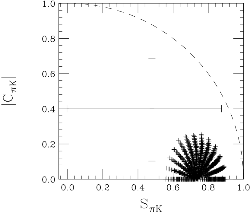
  Figure 2: Points in the $S_{\pi K}$–$|C_{\pi K}|$ plane satisfying $\pm 1\sigma$ limits on the ratio $(1\pm r_{\rm max})^{2}R_{\pi/K}$, where $r_{\rm max}=0.4$, i.e., taking into account upper bound on $\bar{\cal B}(B^{0}\to K^{+}K^{-})$. Other notation is the same as in Fig. 1.

• The process $B^{0}\to\pi^{0}K^{0}$ is related by U-spin to $B_{s}\to\pi^{0}\bar{K}^{0}$ [22], for which the amplitude is given by [14]

  $$A(B_{s}\to\pi^{0}\bar{K}^{0})=(p-c)/\sqrt{2}~{}.$$ (44)

  In the SU(3) limit, this amplitude is equal to $A(B^{0}\to\pi^{0}\pi^{0})+A(B^{0}\to K^{+}K^{-})/\sqrt{2}$ and may replace this sum on the left-hand-side of Eq. (19). In order to obtain bounds on $S_{\pi K}$ and $C_{\pi K}$ as above, one would then have to know the ratio $\bar{\cal B}(B_{s}\to\pi^{0}\bar{K}^{0})/\bar{\cal B}(B^{0}\to\pi^{0}K^{0})$. Measuring the charge averaged rate for $B_{s}\to\pi^{0}\bar{K}^{0}$ in an environment of a hadronic collider may be quite challenging.

• The method for obtaining correlated bounds on $\Delta S_{\pi K}$ and $C_{\pi K}$ may be applied to CP asymmetries in other processes, such as $B^{0}\to\eta^{\prime}K_{S}$ and $B^{0}\to\phi K_{S}$. In [7] upper bounds on quantities analogous to $|c^{\prime}/p^{\prime}|$ were obtained by relating within SU(3) the amplitudes of these processes to the sum of several $\Delta S=0$ amplitudes. For $B^{0}\to\phi K_{S}$, the bound requires an assumption that a term with weak phase $\gamma$ is not much larger than in $B^{+}\to\phi K^{+}$. The SU(3) relations for $B^{0}\to\eta^{\prime}K_{S}$ and $B^{+}\to\phi K^{+}$ were shown to follow from U-spin symmetry [9, 10]. The bounds on a ratio analogous to $|c^{\prime}/p^{\prime}|$ provided estimates for the maximal values of the asymmetries $|S-\sin 2\beta|$. In deriving these bounds additive corrections of order $(\lambda^{2})$ were neglected in quantities resembling $\sqrt{R_{\pi/K}}$, and only leading order terms in a $|c^{\prime}/p^{\prime}|$ expansion were kept. Studying the dependence of the asymmetries $S$ and $C$ on $c^{\prime}/p^{\prime}$, and on strong and weak phases, and avoiding such approximations, one can use the SU(3) relations of [7, 9, 10] in order to get more precise bounds in the $S-|C|$ plane.

We are grateful to Jim Smith for raising a question which motivated this study. M. G. wishes to thank the SLAC theory group for its kind hospitality. The work of Y. G. is supported in part by a grant from GIF, the German–Israeli Foundation for Scientific Research and Development, by the United States–Israel Binational Science Foundation through grant No. 2000133, by the Israel Science Foundation under grant No. 237/01, by the Department of Energy, contract DE-AC03-76SF00515 and by the Department of Energy under grant no. DE-FG03-92ER40689.

References

[1] BaBar Collaboration, B. Aubert et al.,
Phys. Rev. Lett. 89, 201802 (2002);
Belle Collaboration, K. Abe et al., Phys. Rev. D 66, 071102 (2002).
[2] M. Kobayashi and T. Maskawa, Prog. Theor. Phys. 49, 652 (1973).
[3] Particle Data Group, K. Hagiwara et al.,
Phys. Rev. D 66, 010001 (2002).
[4] D. London and R. D. Peccei, Phys. Lett. B 223, 257 (1989);
M. Gronau, Phys. Rev. Lett. 63, 1451 (1989); B. Grinstein,
Phys. Lett. B 229, 280 (1989).
[5] T. Browder, talk presented at LP03 (21st
International Symposium on Lepton and Photon Interactions at
High Energies) Batavia, IL, August 11–16, 2003.
[6] Y. Grossman, G. Isidori and M. P. Worah,
Phys. Rev. D 58, 057504 (1998).
[7] Y. Grossman, Z. Ligeti, Y. Nir and H. R. Quinn,
Phys. Rev. D 68, 015004 (2003).
[8] M. Gronau and J. L. Rosner, Phys. Lett. B 564, 90 (2003).
[9] C. W. Chiang, M. Gronau and J. L. Rosner,
Phys. Rev. D 68, 074012 (2003).
[10] C. W. Chiang, M. Gronau, Z. Luo, J. L. Rosner
and D. A. Suprun, hep-ph/0307395, submitted for publication
in Phys. Rev. D.
[11] Y. Grossman and M. P. Worah, Phys. Lett. B 395, 241 (1997); D. London and A. Soni, Phys. Lett. B 407, 61 (1997).
[12] BaBar Collaboration, A. Farbin et al., PLOT–0053,
contribution to LP03,
Ref. [5];
https://oraweb.slac.stanford.edu:8080/pls/slacquery/
babar_documents.startup.
[13] J. Fry, talk presented at LP03,
Ref. [5]; Updated
results and
references are tabulated periodically by the Heavy
Flavor Averaging Group:
http://www.slac.stanford.edu/xorg/hfag/rare.
[14] M. Gronau, O. Hernández, D. London, and J. L.
Rosner, Phys. Rev. D 50, 4529 (1994).
[15] M. Gronau, O. Hernández, D. London, and
J. L. Rosner,
Phys. Rev. D 52, 6374 (1995). In the present note we are including
in all electroweak
penguin contributions with a common CKM factor ,
using a somewhat different definition than in the above paper.
[17] M. Gronau and J. L. Rosner,
Phys. Rev. D 58, 113005 (1998).
[18] A. Höcker et al., Eur. Phys. J. C 21, 225 (2001).
Updated results
may be found on the web site http://ckmfitter.in2p3.fr.
[19] M. Beneke, G. Buchalla, M. Neubert and C.
T. Sachrajda, Nucl. Phys. B 606, 245 (2001); M. Beneke and M. Neubert,
hep-ph/0308039. SU(3) breaking effects relating
and were studied recently
by M. Beneke, hep-ph/0308040.
[20] Y. Y. Keum, H. N. Li and A. I. Sanda,
Phys. Lett. B 504, 6 (2001).
[21]
Y. Grossman, M. Neubert and A. L. Kagan,
JHEP 9910, 029 (1999);
T. Yoshikawa, hep-ph/0306147; M. Gronau
and J. L. Rosner, Phys. Lett. B 572, 43 (2003); A. J. Buras, R.
Fleischer, S. Recksiegel and F. Schwab, hep-ph/0309012.