The trilinear neutral Higgs self-couplings
in the MSSM.
Complete one-loop analysis

Abstract

The Higgs boson effective self-couplings $\lambda_{hhh}$ and $\lambda_{HHH}$ are calculated in the framework of the Minimal Supersymmetric Standard Model (MSSM) for the complete set of one-loop diagrams with one of the Higgs bosons off-shell. The comparison with previous results, where only the leading correction terms in the limiting case of large masses of virtual particles were calculated, is carried out. We analyse the dependence of the self-couplings on the energy and ${\tt tan}\beta$; it is demonstrated that the tree-level self-couplings could acquire substantial one-loop corrections, which could be phenomenologically important.

Introduction

Two basic elements of the gauge boson and fermion mass generation in the Standard Model (SM) and its minimal supersymmetric extension (MSSM) are (1) the spontaneous symmetry breaking (SSB) [1] and (2) the Higgs mechanism [2]. Gauge bosons and fermions gain masses via gauge-invariant interaction with scalar fields, which have non-zero vacuum expectation values. The SSB and Higgs mechanism respect gauge invariance and renormalizability of the model. In order to confirm experimentally the mechanism of mass generation, it is needed (1) to detect the Higgs bosons and measure their masses (2) to measure the Higgs boson couplings with gauge bosons and fermions (3) to determine the Higgs boson self-couplings. The last step is important especially for the case of MSSM, where the self-couplings are determined by the soft supersymmetry breaking principle. Tree-level analysis shows that some neutral Higgs boson self-couplings can be measured [3, 4, 5] with relatively high accuracy on the future high-luminosity colliders. The leading one-loop corrections to the neutral Higgs self-couplings may be expected to be sizable in some regions of MSSM parameter space, with the potential to change substantially the tree-level results.

We calculate two self-couplings of the neutral MSSM Higgs bosons $h^{0}$, $H^{0}$ taking into account the complete set of one-loop diagrams. Our main interest is the analysis of modifications in the Higgs potential by the corrections coming from the scalar and sparticle sectors of the model.

In section 1 the Higgs boson interaction Lagrangian and the self-couplings are presented. In sections 2 and 3 we discuss technical details of the approach. Some numerical results and their comparative analysis are contained in section 4.

1 Higgs boson interaction Lagrangian

The Higgs sector of MSSM includes five physical fields:

$\diamond$ two neutral $CP-$ even Higgs fields $\{h^{0},H^{0}\}$;

$\diamond$ neutral $CP-$ odd Higgs field $A^{0}$;

$\diamond$ charged fields $H^{\pm}$.

The Higgs boson interaction Lagrangian has the form

$$\mathcal{L}_{Int}^{Higgs}=\mathcal{L}_{Int}^{(3)}+\mathcal{L}_{Int}^{(4)}$$ (1)

$\mathcal{L}_{Int}^{(3)}-$ Lagrangian of the triple Higgs boson interactions,
$\mathcal{L}_{Int}^{(4)}-$ Lagrangian of the quartic Higgs boson interactions.

$$\mathcal{L}_{Int}^{(3)}=\frac{\lambda_{hhh}}{3!}hhh+\frac{\lambda_{hhH}}{2!}hhH+\frac{\lambda_{hHH}}{2!}hHH+$$

$$\frac{\lambda_{HHH}}{3!}HHH+\frac{\lambda_{hAA}}{2!}hAA+\frac{\lambda_{HAA}}{2!}HAA+$$

$$\lambda_{hH^{+}H^{-}}hH^{+}H^{-}+\lambda_{HH^{+}H^{-}}HH^{+}H^{-}$$ (2)

The tree level Higgs boson self-couplings are represented in (2) as functions of the two free parameters: mass of Higgs field $A^{0}$, $M_{A}$ and mixing angle $\beta$.

$$\lambda_{hhh} = -3ia_{0}\cos(2\alpha)\sin(\alpha+\beta)$$ (3)

$$\lambda_{hhH} = -ia_{0}[2\sin(2\alpha)\sin(\alpha+\beta)-\cos(2\alpha)\cos(\alpha+\beta)]$$ (4)

$$\lambda_{hHH} = ia_{0}[2\sin(2\alpha)\cos(\alpha+\beta)+\cos(2\alpha)\sin(\alpha+\beta)]$$ (5)

$$\lambda_{HHH} = -3ia_{0}\cos(2\alpha)\cos(\alpha+\beta)$$ (6)

$$\lambda_{hAA} = -ia_{0}\cos(2\beta)\sin(\alpha+\beta)$$ (7)

$$\lambda_{HAA} = ia_{0}\cos(2\beta)\cos(\alpha+\beta)$$ (8)

$$\lambda_{hH^{+}H^{-}} = -igM_{W}\sin(\beta-\alpha)-ia_{0}\cos(2\beta)\sin(\alpha+\beta)$$ (9)

$$\lambda_{HH^{+}H^{-}} = -igM_{W}\cos(\beta-\alpha)-ia_{0}\cos(2\beta)\cos(\alpha+\beta)$$ (10)

where $M_{W}$, $M_{Z}$ - gauge boson masses, $\theta$ - Weinberg angle, $g$ - $SU(2)_{L}$ gauge constant. Connections between the mixing angles $\alpha$ and $\beta$ and also the parameter $a_{0}$ are determined by the conditions

$$\tan 2\alpha=\tan 2\beta\frac{M_{A}^{2}+M_{Z}^{2}}{M_{A}^{2}-M_{Z}^{2}},\hskip 11.38109pta_{0}=\frac{igM_{z}}{2\cos(\theta_{W})}$$ (11)

2 Perturbation theory. Vertex function

Main object of our study is the vertex function (VF) of the triple Higgs interaction.

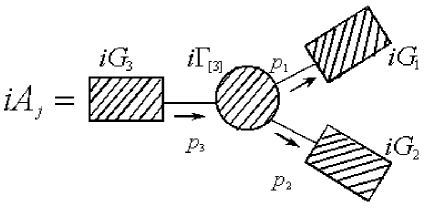
Figure 1: Feynman diagram for amplitude $A_{j}$.

Following the standard normalization conventions [7, 8], the amplitude of the given diagram can be represented as follows (see Fig. 1):

$$-iA_{j}=-iG_{1}(p_{1},\{a_{1}\})(i\Gamma_{[3]}(p_{1},p_{2},p_{3},\{c\}))G_{2}(p_{2},\{a_{2}\})G_{3}(p_{3},\{a_{3}\})$$ (12)

where $G_{i}(p_{i},\{a_{i}\})$ – the Green’s functions beyond the given diagram, $p_{i}$ –  the four-vector of $i-th$ Higgs boson. $\{a\},\{c\}$ – sets of model parameters, characterizing given diagram. $\Gamma_{[3]}(p_{1},p_{2},p_{3},\{c\})$ – vertex function of the triple Higgs interaction. It can be represented as

$$\Gamma_{[3]}(p_{1},p_{2},p_{3},\{c\})=\sum_{l=0}^{\infty}\Gamma_{[3]}^{(l)}(p_{1},p_{2},p_{3},\{c\})$$ (13)

In the last expression the decomposition in $\alpha_{e}$ is performed. Each term coincides with the sum of one-particle irreducible diagrams of the order of $\alpha_{e}$. Our analysis is carried out for the decomposition

$$\Gamma_{[3]}(p_{1},p_{2},p_{3},\{c\})=\Gamma_{[3]}^{(0)}(p_{1},p_{2},p_{3},\{c\})+\Gamma_{[3]}^{(1)}(p_{1},p_{2},p_{3},\{c\})$$ (14)

Graphical interpretation of the last formula is shown in Fig. 2.

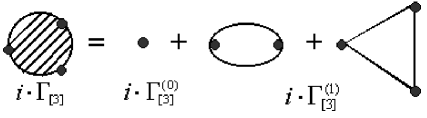
Figure 2: Vertex function decomposition: the one-loop approximation

The condition (13) in terms of self-couplings has the form

$$\lambda_{Hg_{1}Hg_{2}Hg_{3}}=\lambda_{Hg_{1}Hg_{2}Hg_{3}}^{(0)}+\Delta\lambda_{Hg_{1}Hg_{2}Hg_{3}}^{(1)}=\lambda_{Hg_{1}Hg_{2}Hg_{3}}^{(0)}(1+\alpha_{e}\Delta\tilde{\lambda}_{Hg_{1}Hg_{2}Hg_{3}}^{(1)})$$ (15)

The complete one-loop contribution (Feynman gauge) is determined by contributions of physical fields (standard fermions, sfermions, gauge bosons, chargino, neutralino), as well as Goldstone modes and gost fields.

$$\Delta\lambda_{Hg_{1}\,Hg_{2}\,Hg_{3}}^{(1)}=\Delta\lambda^{(1)}(f)+\Delta\lambda^{(1)}(\tilde{f})+\Delta\lambda^{(1)}(Gb)+\Delta\lambda^{(1)}(Ch)+$$

$$\Delta\lambda^{(1)}(Neu)+\Delta\lambda^{(1)}(Hg)+\Delta\lambda^{(1)}(Gs)+\Delta\lambda^{(1)}(Gh)$$ (16)

The following analysis is based on the general formulas for the one-loop contributions to two- and three-point vertex functions. Our algorithms are implemented in the computer algebra programs that allow to operate with bulky intermediate expansions.

3 Scheme of calculations

Main features of our calculation are

1. The center-of-mass frame is used for explicit phase space formulas, when one Higgs boson is a virtual particle.

2. Feynman gauge was used.

3. The solutions of renormalization group equations for gauge constants and third generation quarks masses were employed to take into account the energy dependence more precisely [9].

4. Tensor reduction for the scalar one-loop integrals was used [10].

5. On-shell renormalization procedure was employed [11].

The experimental data were taken from [12].

4 Results and their analysis

Two types of dependences are represented in this paper: Higgs self-couplings dependences on $\tan\beta$, $\sqrt{s}$.

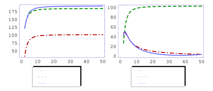
Figure 3: Dependence of the trilinear Higgs self-couplings (on the tree and one-loop levels) on $\tan\beta$, for $\sqrt{s}=m_{Hg_{1}}+m_{Hg_{2}}+10$ GeV, $M_{A}=500$ GeV, $M_{3}=\mu=300$ GeV, $M_{\tilde{Q}}=M_{\tilde{U}}=M_{\tilde{D}}=M_{\tilde{R}}=M_{\tilde{L}}=1$ TeV, $A_{f}=200$ GeV.

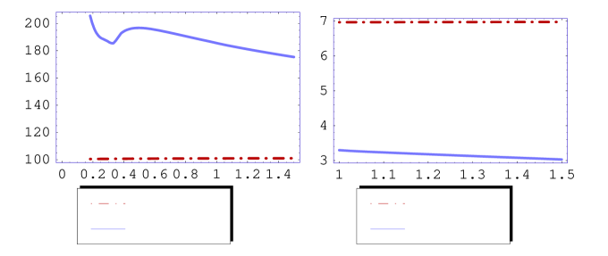
Figure 4: Dependence of the trilinear Higgs self-couplings (on the tree and one-loop levels) on $\sqrt{s}$, for $\tan\beta=30$, $M_{A}=500$ GeV, $M_{3}=\mu=300$ GeV, $M_{\tilde{Q}}=M_{\tilde{U}}=M_{\tilde{D}}=M_{\tilde{R}}=M_{\tilde{L}}=1$ TeV, $A_{f}=200$ GeV.

In Fig. 3 three kinds of dependences on $\tan\beta$ are represented: tree-level self-couplings ($\lambda^{0}$), self-couplings with leading $t-\tilde{t}$ one-loop correction ($\lambda^{0}+\Delta\lambda^{Lead}$) and self-couplings with complete one-loop contribution ($\lambda^{0}+\Delta\lambda^{Comp}$). Analytic expressions for ($\Delta\lambda^{Lead}$) can be found in [6] in the case of large mass approximation for virtual particles.

Obviously, differences between ($\lambda_{hhh}^{0}+\Delta\lambda_{hhh}^{Lead}$) and ($\lambda_{hhh}^{0}+\Delta\lambda_{hhh}^{Comp}$) are insignificant (9.5 % from curve ($\lambda_{hhh}^{0}+\Delta\lambda_{hhh}^{Lead}$) for $\tan\beta=45$). It is important to note that the sizable value of correction does not contradict the perturbation theory applicability.

In [13] it was shown that the self-coupling ($\lambda_{hhh}^{0}+\Delta\lambda_{hhh}^{Comp}$) in the decoupling limit (our situation for $M_{A}=500$ GeV satisfy this limit) can be represented in terms of Higgs boson $h^{0}$ mass. By redefinition of ($\lambda_{hhh}^{0}+\Delta\lambda_{hhh}^{Lead}$) the correction value is being insignificant and do not exceed $6\%$. The analogous conditions for ($\lambda_{hhh}^{0}+\Delta\lambda_{hhh}^{Comp}$) give the correction of $11\%$. Another situation is observed in $\lambda_{HHH}-$ case. The curve coinciding to ($\lambda_{HHH}^{0}+\Delta\lambda_{HHH}^{Lead}$) demonstrates huge one-loop leading contribution in $\lambda_{HHH}$, however the complete one-loop contribution is very small. The reason of this discrepancy is in the usage of the large masse approximation for virtual particles. We have not used any approximations for one-loop scalar integrals. The applicability of the large masse approximation is from our point of view questionable in the situation under consideration (maybe except the $hhh$ - case) because of too large masses of virtual Higgs bosons.

In Fig. 4 the self-couplings dependences on the process energy passing by virtual Higgs boson are represented. One can observe that $\lambda_{HHH}$ is very weekly dependent on $\sqrt{s}$. For a given situation a future high-luminosity colliders can not detect these dependences because we can certainly suppose that $\lambda_{HHH}$ is not a running parameter. Another situation is observed in $\lambda_{hhh}-$ case. For instance for $\sqrt{s}=186$ GeV the self-coupling $\lambda_{hhh}=205$ GeV and for $\sqrt{s}=1500$ GeV the self-coupling $\lambda_{hhh}=175$ GeV. If the accuracy of the self-coupling measurement on the future colliders will be better than 30 GeV, that given dependence could be detected.

The summing error of results is determined by determination error of $t-$ quark mass ($\delta m=5.1$ GeV) and by generality of soft supersymmetry breaking parameters values. Errors for $\lambda_{hhh}-$ case are equal 5 GeV and 8 GeV, and for $\lambda_{HHH}-$ case 1 GeV and 2 GeV accordingly (for $M_{A}=500$ GeV).

Conclusion

In this work the neutral Higgs boson self-couplings with complete set of the one-loop diagrams are represented and analyzed in the framework of the MSSM. The effective dependences of the Higgs boson self-couplings $\lambda_{hhh}$, $\lambda_{HHH}$ on $\tan\beta$ and energy $\sqrt{s}$ are evaluated with one of the Higgs bosons is off-shell. The authors have avoided any approximations in one-loop scalar integrals calculations. It has been shown, that the tree-level self-couplings can acquire sizable one-loop corrections. These must be taken into account for detailed comparative analysis of theory and experimental data, which could be phenomenologically important.

References

- [1] J. Goldstone - Nuovo Cimento, v19 154, (1961); Y. Nambu, G. Jona-Lasinio - Phys. Rev., v122 345,(1961); J. Goldstone, A. Salam, S. Weinberg - Phys. Rev., v127 965,(1962);
- [2] P.W. Higgs Phys. Lett., 12 132 (1964); E. Englert, R. Brout Phys. Rev. Lett., 13 321 (1964); P.W. Higgs Phys. Rev. Lett., 13 508 (1964); G.S. Guralnik, C.R. Hagen, T.W.B. Kibble Phys. Rev. Lett., 13 585 (1964); P.W. Higgs Phys. Rev., v145 1156 (1966); T.W.B. Kibble Phys. Rev., v155 1554 (1967);
- [3] R.M. Zerwas, hep-ph/0003221.
- [4] A. Djouadi, W. Kilian, M. Muhlleitner, P.M. Zerwas, hep-ph/0001169, DESY 99/171.
- [5] S.Dawson, hep-ph/9912433.
- [6] H.E. Haber, and R. Hempfling, Phys. Rev. Lett. 66 1815, (1991); Y. Okada, M. Yamaguchi, T. Yanagida, Prog. Theor. Phys. 85 1, (1991); J. Ellis, G. Ridolfi and F. Zwirner, Phys. Lett. B257 83, (1991). V.Barger, M.S. Berger, A.L. Stange and R.J.N. Phillips, Phys. Rev. D45 4128, (1992); Z.Kunszt and F. Zwirner, Nucl. Phys. B385 3, (1992) . A. Djouadi, H.E. Haber, P.M. Zerwas, Phys. Lett. B375 203, (1996).
- [7] By N.N. Bogolyubov, D.V. Shirkov, Introduction to the theory of quantized fields. (Steklov Math. Inst., Moscow Dubna, JINR). Published in Intersci.Monogr.Phys.Astron. 3 1,(1959).
- [8] V. B. Berestetskii, L.D. Landau, E.M. Lifshitz, L. P. Pitaevskii, Quantum Electrodynamics, 2nd ed. Oxford, England: Pergamon Press, (1982).
- [9] H.E. Haber, R. Hempfling, A.H. Hoang, hep-ph/9609331.
- [10] L.M. Brown, R.P. Feynman, Phys.Rev., 85 231, (1952); G. Passarino, M.J.G. Veltman, Nucl.Phys., B160 151, (1979).
- [11] P.H. Chankovski, S. Pokorski, J. Rosiek, Nucl. Phys., B423 437, (1994); A. Dabelstein, Z. Phys., C67 495, (1995), Nucl. Phys., B456 25, (1995).
-
[12]
LEP EWWG, http://lepewwg.web.cern.ch/LEPEWWG/plots
/summer2000/;
D.E.Groom et. al, Eur. Phys. J. c15 1, (2000);
S. Bethke, J. Phys. G26 R27, (2000);
A.D. Martin, J.Outhwaite, M.C. Ryskin, Phys. Lett. B492 69, (2000). - [13] W.Hollik, S. Penaranda, Eur.Phys.J.C23 163, (2002).