Relativistic Faddeev approach to a non-local NJL model

Abstract

The diquark and nucleon are studied in a non-local NJL model. We solve the relativistic Faddeev equation and compare the results with the ordinary NJL model. Although the model is quark confining, it is not diquark confining in the rainbow-ladder approximation. We show that the off-shell contribution to the diquark $T$ matrix is crucial for the structure of the nucleon: without its inclusion the attraction in the scalar channel is too weak to form a three-body bound state.

1 Introduction

The NJL model is a successful low-energy phenomenological model inspired by QCD njl . It has also been applied to the nucleon, see Refs. njln . However, the lack of confinement makes the model questionable in the baryonic sector. It has been shown that a non-local covariant extension of this model can lead to quark confinement for acceptable values of the parameters pb . This occurs due to the fact that the quark propagator has no real poles, and consequently quarks do not appear as asymptotic states. There are several other advantages of the non-local version over the local NJL model: the non-locality regularises the model in a manner such that anomalies and gauge invariance are preserved and the momentum-dependent regulator makes the theory finite to all orders in the $1/N_{c}$ expansion. Finally the dynamical quark mass is momentum dependent in contrast to the ordinary NJL model and consistent with lattice simulations of QCD. As a result, the non-local version of the NJL model may have more predictive power.

Here we shall use the covariant quark-diquark formalism in a relativistic Faddeev equation for the nucleon, where we include only scalar diquark correlations. Due to the separability of the non-local interaction, the Faddeev equations can be reduced to a set of effective Bethe-Salpeter equations. This makes it possible to adopt the numerical method developed for such problems by Oettel et al. o .

2 The Model

We consider a non-local NJL model Lagrangian with $SU(2)_{f}\times SU(3)_{c}$ symmetry. There exists several versions of such non-local NJL models. Regardless of what version is chosen, a Fierz transformation allows one to rewrite the interaction in either the $q\bar{q}$ or $qq$ channels. Here we truncate to the scalar ($0^{+},T=0$) and pseudoscalar ($0^{-},T=1$) mesonic channels. To investigate the nucleon in the quark-diquark picture, one also needs to know the $qq$ interaction. We truncate to the scalar ($0^{+},T=0$) colour $\overline{3}$ $qq$ channel,

$$\mathcal{L}_{I\pi} = \frac{1}{2}g_{\pi}j_{\alpha}(x)j_{\alpha}(x),\hskip 56.9055pt\mathcal{L}_{Is}=g_{s}\overline{J}_{s}(x)J_{s}(x),$$

$$j_{\alpha}(x) = \int d^{4}x_{1}d^{4}x_{3}f(x-x_{3})f(x_{1}-x)\overline{\psi}(x_{1})\Gamma_{\alpha}\psi(x_{3}),$$

$$\overline{J}_{s}(x) = \int d^{4}x_{1}d^{4}x_{3}f(x_{1}-x)f(x-x_{3})\overline{\psi}(x_{1})\big{[}\gamma_{5}C\tau_{2}\beta^{A}\big{]}\overline{\psi}^{T}(x_{3}),$$

$$J_{s}(x) = \int d^{4}x_{2}d^{4}x_{4}f(x_{2}-x)f(x-x_{4})\psi^{T}(x_{2})\big{[}C^{-1}\gamma_{5}\tau_{2}\beta^{A}\big{]}\psi(x_{4}).\$$ (1)

Here $\Gamma_{\alpha}=(1,i\gamma_{5}\tau)$ and $m_{c}$ is the current quark mass of the $u$ and $d$ quarks. The matrices $\beta^{A}=\sqrt{3/2}\lambda^{A}(A=2,5,7)$ project onto the colour $\overline{3}$ channel with normalisation $\operatorname{tr}(\beta^{A}\beta^{A^{\prime}})=3\delta^{AA^{\prime}}$ and the ${\tau_{i}}$’s are flavour $SU(2)$ matrices with $\operatorname{tr}(\tau_{i}\tau_{j})=2\delta_{ij}$. The object $C=i\gamma_{2}\gamma_{5}$ is the charge conjugation matrix. Since we do not restrict ourselves to specific choice of interaction, we shall treat the couplings $g_{s}$ and $g_{\pi}$ as independent. For simplicity, we assume the form factor $f(x-x_{i})$ to be local in momentum space, since it leads to a separable interaction in momentum space.

The dressed quark propagator $S(k)$ is now constructed by means of a Schwinger-Dyson equation (SDE) in rainbow-ladder approximation. Thus the dynamical constituent quark mass, arising from spontaneously broken chiral symmetry, is obtained as [the symbol $\operatorname{Tr}$ denotes a trace over flavour, colour and Dirac indices]

$$m(p)=m_{c}+ig_{\pi}f^{2}(p)\int\frac{d^{4}k}{(2\pi)^{4}}\operatorname{Tr}[S(k)]f^{2}(k),\hskip 28.45274ptS^{-1}(k)=\not{k}-m(k).$$ (2)

Following Ref. pb , we choose the form factor to be Gaussian in Euclidean space, $f(p_{E})=\exp(-p_{E}^{2}/\Lambda^{2})$, where $\Lambda$ is a cutoff of the theory. If one assumes that $\Lambda$ is related to the average inverse size of instantons $1/\bar{\rho}$, its choice thus parametrises non-perturbative properties of the QCD vacuum. The choice (2) respects Poincaré invariance and leads to quark, but not colour, confinement, when the dressed quark propagator has no poles at real $p^{2}$ in Minkowski space. This occurs for

$$\frac{m(0)-m_{c}}{\sqrt{m^{2}_{c}+\Lambda^{2}}-m_{c}}>\frac{1}{2}\exp\left(-\frac{(\sqrt{m^{2}_{c}+\Lambda^{2}}+m_{c})^{2}}{2\Lambda^{2}}\right).$$ (3)

For large enough values of the dynamical quark mass, the quark propagator has no real poles and quarks do not appear as asymptotic states. The propagator still has infinitely many pairs of complex poles, both for confining and non-confining parameter sets. This is a feature of such models and due care should be taken in handling such poles, which can not be associated with asymptotic states if the theory is to satisfy unitary.

Our model has four free parameters: the current quark mass $m_{c}$, the cutoff ($\Lambda$), the coupling constants $g_{\pi}$ and $g_{s}$. We fix the first three to give a pion mass of $136.6$ MeV with decay constant of $92.4$ MeV, as the value of the zero-momentum quark mass in chiral limit $m_{0}(0)$. We analyse three sets of parameters, as indicated in table 1. Set $A$ is non-confining and sets $B$ and $C$ are confining (i.e., they satisfy the condition Eq. (3)). The parameter $g_{s}$ is not constrained by these conditions, which allows us to analyse the coupling constant dependence through the ratio $r_{s}=g_{s}/g_{\pi}$.

Parameter	set A	set B	set C
$m_{0}(0)$ (MeV)	250	350	400
$m(0)$ (MeV)	297.9	406.2	461.3
$m_{c}$ (MeV)	7.9	14.4	17.6
$\Lambda$ (MeV)	1046.8	723.4	638.1
$g_{\pi}(\text{ GeV}^{-2})$	31.6	89.0	132.6

Table 1: The model parameters for different sets, fitted as discussed in text. The resulting value of the dynamical quark mass $m(0)$ also is shown.

3 Diquark and Nucleon solution

In the rainbow-ladder approximation the diquark $T$-matrix can be written as

$$T(p_{1},p_{2},p_{3},p_{4}) = f(p_{1})f(p_{3})\big{[}\gamma_{5}C\tau_{2}\beta^{A}\big{]}t(q)\big{[}C^{-1}\gamma_{5}\tau_{2}\beta^{A}\big{]}f(p_{2})f(p_{4})$$ (4)

$$\times\delta(p_{1}+p_{2}-p_{3}-p_{4}),\$$

where $q=p_{1}-p_{3}=p_{4}-p_{2}$ and

$$t(q) = \frac{2g_{s}i}{1+g_{s}J_{s}(q)},$$ (5)

$$J_{s}(q) = i\operatorname{Tr}\int\frac{d^{4}k}{(2\pi)^{4}}f^{2}(-k)\big{[}\gamma_{5}C\tau_{2}\beta^{A}\big{]}S(-k)^{T}\big{[}C^{-1}\gamma_{5}\tau_{2}\beta^{A}\big{]}S(q+k)f^{2}(q+k).\$$ (6)

In the above equation the quark propagators are the solution of the rainbow SDE Eq. (2). The diquark bound state is located at the pole of the $T$-matrix. The denominator of Eq. (5) is the same as that in pionic channel, thus one may conclude that at $r_{s}=1$ the diquark and pion are degenerate. This puts an upper limit to the choice of $r_{s}$, since diquarks should not to condense in vacuum.

The relativistic Faddeev equation can be written as an effective two-body BSE between a quark and a diquark due to the separability of the two-body interaction in momentum-space. Using the the on-shell approximation this becomes an eigenvalue problem o ,

$$\int\frac{d^{4}k}{(2\pi)^{4}}K_{\alpha\gamma}(p,k;P)\psi_{\gamma\beta}(k,P)=\lambda(P^{2})\phi_{\alpha\beta}(p,P),$$ (7)

$$\psi(p,P)=S(p_{q})D(p_{d})\phi(p,P),$$ (8)

$$K(p,k;P)=\frac{2}{g_{dqq}^{2}}X(P_{1})S^{T}(q)\overline{X}(P_{2}).\$$ (9)

Here $\psi(p,P)$ is the nucleon bound-state wave function related to the vertex function $\phi(p,P)$ by truncation of the legs. The parameters $p$ and $P$ are the relative and total momenta in the quark-diquark system, respectively. We define $p_{q}=\eta P+p$, $p_{d}=(1-\eta)P-p$ and $q=-p-k+(1-2\eta)P$. The relative momentum of quarks in the diquark vertices $X$ and $\overline{X}$ are defined as $p_{1}=p+k/2-(1-3\eta)P/2$ and $p_{2}=-k-p/2+(1-3\eta)P/2$ respectively. (For $\eta$ see below.)

These equations should be solved for the largest eigenvalue of $\lambda(P^{2})$ with the constraint that $\lambda(P^{2})=1/g^{2}_{dqq}$ at $P^{2}=M^{2}_{N}$, where $M_{N}$ is nucleon mass. Here $g_{dqq}$ denotes the diquark-quark interaction coupling, $g_{dqq}^{-2}=\left(\partial_{k^{2}}J_{s}\right)|_{k^{2}=M_{d}^{2}}$, where $J_{s}$ is defined in Eq. (6). In the usual on-shell approximation the scalar diquark propagator is taken to be $D(p_{d})^{-1}=-(p_{d}^{2}+M_{d}^{2})$ where $M_{d}$ is the pole of the scalar diquark $T$-matrix. The functions $X$ and its adjoint $\overline{X}=\gamma_{0}X^{{\dagger}}\gamma_{0}$ are the vertex functions of two quarks within the diquark and can be obtained from Eq. (4),

$$X(p_{1},k_{d})=g_{dqq}\gamma_{5}C\tau_{2}\beta^{A}f(p_{1}+(1-\sigma)k_{d})f(-p_{1}+\sigma k_{d}).$$ (10)

The non-locality of our model naturally leads to an extended diquark, and provides a sufficient regularisation of the ultraviolet divergences for a diquark-quark loop. Above we have introduced the Mandelstam parameters $\eta$ and $\sigma$, $\eta,\sigma\in[0,1]$. In principle, the eigenvalues should not depend on these parameters if the formulation is Lorentz covariant. However, in practise due to numerical errors and singularities in the propagators, one usually only finds that there are substantial plateaus where the results are $\eta$- and $\sigma$-independent. The nucleon vertex function $\phi(p,P)$ should correspond to a state of positive energy, positive parity and spin-$1/2$. This leads to the general structure

$$\phi(p,P)=\left(S_{1}+\frac{i}{M_{N}}\not{p}S_{2}\right)\Lambda^{{\dagger}},$$ (11)

where $\Lambda^{{\dagger}}=\frac{1}{2}(1+\frac{\not{P}}{iM_{N}})$ is a positive energy projection for a nucleon with mass $M_{N}$, and $S_{1}$ and $S_{2}$ are scalar function. We now solve the equations in the rest frame of the nucleon. We expand the scalar functions in terms of Chebyshev polynomials of the first kind, which turns out to be very efficient for such problems o .

4 Results

The scalar diquark mass $M_{D}$ is obtained as a pole of Eq. (5). We find that for a wide range of $r_{s}$, regardless of the parameter set and confinement, a bound scalar diquark exists. The diquark masses for various value of $r_{s}$ for different parameter sets are plotted in Fig. 1a. For sets A, B, C no bound scalar diquark exists for $r_{s}<0.110,0.112,0.146$, respectively. Please note that the confinement of the diquark for very small $r_{s}$ is due to the screening effect of the ultraviolet cutoff and should not be associated to the underlying QCD confinement which stems from infrared divergence of gluon and ghost propagators. Having said that it is possible that diquark confinement may arise beyond the rainbow-ladder approximation new .

In order to solve the Faddeev equation numerically, we have first used the on-shell approximation. We observe that one can not generate a three-body bound state in this model, without an artificial enhancement of the quark-diquark coupling of about 3. A similar feature has been observed in the ordinary NJL model as well njln , but the effect is even more severe here. As can be seen from Fig. 1 a decrease in $r_{s}$ leads to a larger diquark mass, and an increase in the off-shell contribution to the $qq$ $T$-matrix. It is this off-shell contribution that leads to a bound nucleon, and they are indeed substantial as can be seen in Fig. 1b. A preliminary result is shown in Fig. 1c. We also show a fictitious diquark-quark threshold defined as $M_{qq}+m_{q}^{\text{p}}$, where $m_{q}^{\text{p}}$ is the real part of the first pole of quark propagator. Given this definition the diquarks in the nucleon are much more loosely bound in the non-local model than in the ordinary NJL model. Nonetheless, we obtain a bound nucleon solution near its experimental value.

The research of NRW and MCB was supported by the UK EPSRC; AHR acknowledges the award of an ORS studentship.

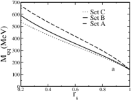
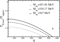
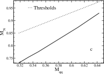
Figure 1: (a) Shows the diquark masses with respect to $r_{s}$ for three sets of parameters. (b) Shows the discrepancy between the on- and off-shell approximation for three diquark masses (parameter set B). In (c) the nucleon mass is shown as a function of diquark mass for set B, the values are given in GeV.

References

- (1) J. Bijnens, Phys. Rept. 265, 369 (1996).
- (2) A. Buck, R. Alkofer and H. Reinhardt, Phys. Lett. B286, 29 (1992); S. Huang and J. Tjon, Phys. Rev. C49, 1702 (1994); W. Bentz, H. Mineo, H. Asami, K. Yazaki, Nucl. Phys. A670, 48 (2000).
- (3) R. D. Bowler and M. C. Birse, Nucl. Phys. A582, 655 (1995); R. S. Plant and M. C. Birse, Nucl. Phys. A628, 607 (1998).
- (4) M. Oettel, L. Von Smekal, R. Alkofer, Comput. Phys. Commun. 144, 63 (2002); M. Oettel, R. Alkofer, L. von Smekal, Eur. Phys. J. A8, 553 (2000); M. Oettel, G. Hellstern, R. Alkofer, H. Reinhardt, Phys. Rev. C58, 2459, (1998).
- (5) A. Bender, C. D. Roberts and L. V. Smekal, Phys. Lett B380, 7 (1997); G. Hellstern, R. Alkofer and H. Reinhardt, Nucl. phys. A625, 697 (1997).