Parton Distributions

Abstract

I discuss our current understanding of parton distributions. I begin with the underlying theoretical framework, and the way in which different data sets constrain different partons, highlighting recent developments. The methods of examining the uncertainties on the distributions and those physical quantities dependent on them is analysed. Finally I look at the evidence that additional theoretical corrections beyond NLO perturbative QCD may be necessary, what type of corrections are indicated and the impact these may have on the uncertainties.

1 Introduction

The proton is described by QCD – the theory of the strong interactions. This makes an understanding of its structure a difficult problem. However, it is also a very important problem – not only as a question in itself, but also in order to search for and understand new physics. Many important particle colliders use hadrons – HERA is an $ep$ collider, the Tevatron is a $p\bar{p}$ collider, the LHC at CERN will be a $pp$ collider, and an understanding of proton structure is essential in order to interpret the results. Fortunately, when one has a relatively large scale in the process, in practice only $>1{\rm GeV}^{2}$, the proton is essentially made up of the more fundamental constituents – quarks and gluons (partons), which interact relatively weakly. Hence, the fundamental quantities one requires in the calculation of scattering processes involving hadronic particles are the parton distributions. These can be derived from, and then used within, the factorization theorem which separates processes into nonperturbative parts which can be determined from experiment, and perturbative parts which can be calculated as a power-series in the strong coupling constant $\alpha_{S}$.

This is illustrated in the canonical example of deep inelastic scattering. The cross-section for the virtual photon-proton interaction can be written in the factorized form

$$\sigma(ep\to eX)=\sum_{i}C^{DIS}_{i}(x,\alpha_{s}(Q^{2}))\otimes f_{i}(x,Q^{2})$$

where $Q^{2}$ is the photon virtuality, $x=\frac{Q^{2}}{2m\nu}$, the momentum fraction of parton ($\nu$=energy transfer in the lab frame), and the $f_{i}(x,Q^{2})$ are the parton distributions, i.e the probability of finding a parton of type $i$ carrying a fraction $x$ of the momentum of the hadron. Corrections to the above formula are of ${\cal O}(\Lambda_{{\rm QCD}}^{2}/Q^{2})$ and are known as higher twist. The parton distributions are not easily calculable from first principles. However, they do evolve with $Q^{2}$ in a perturbative manner, satisfying the evolution equation

$$\frac{df_{i}(x,Q^{2})}{d\ln Q^{2}}=\sum_{i}P_{ij}(x,\alpha_{s}(Q^{2}))\otimes f_{j}(x,Q^{2})$$

where the splitting functions $P_{ij}(x,\alpha_{s}(Q^{2}))$ are calculable order by order in perturbation theory. The coefficient functions $C^{P}_{i}(x,\alpha_{s}(Q^{2}))$ describing a hard scattering process are process dependent but are calculable as a power-series, i.e $C^{P}_{i}(x,\alpha_{s}(Q^{2}))=\sum_{k}C^{P,k}_{i}(x)\alpha^{k}_{s}(Q^{2}).$ Since the $f_{i}(x,Q^{2})$ are process-independent, i.e. universal, once they have been measured at one experiment, one can predict many other scattering processes.

Global fits[1]^-[7] use all available data, largely structure functions, and the most up-to-date QCD calculations, currently NLO–in–$\alpha_{s}(Q^{2})$, to best determine these parton distributions and their consequences. In the global fits input partons are parameterized as, e.g.

$$xf(x,Q_{0}^{2})=(1-x)^{\eta}(1+\epsilon x^{0.5}+\gamma x)x^{\delta}$$

at some low scale $Q_{0}^{2}\sim 1-5{\rm GeV}^{2}$, and evolved upwards using NLO evolution equations. Perturbation theory should be valid if $Q^{2}>2{\rm GeV^{2}}$, and hence one fits data for scales above $2-5{\rm GeV}^{2}$, and this cut should also remove the influence of higher twists, i.e. power-suppressed contributions.

In principle there are many different parton distributions – all quarks and antiquarks and the gluons. However, $m_{c},m_{b}\gg\Lambda_{{\rm QCD}}$ (and top does not usually contribute), so the heavy parton distributions are determined perturbatively. Also we usually assume $s=\bar{s}$, and that isospin symmetry holds, i.e. $p\to n$ leads to $d(x)\to u(x)$ and $u(x)\to d(x)$. This leaves 6 independent combinations. Relating $s$ to $1/2(\bar{u}+\bar{d})$ we have the independent distributions

$$u_{V}=u-\bar{u},\,d_{V}=d-\bar{d},\,{\rm sea}=2*(\bar{u}+\bar{d}+\bar{s}),\,\bar{d}-\bar{u},\,g.$$

It is also convenient to define $\Sigma=u_{V}+d_{V}+{\rm sea}+(c+\bar{c})+(b+\bar{b})$. There are then various sum rules constraining parton inputs and which are conserved by evolution order by order in $\alpha_{S}$, i.e. the number of up and down valence quarks and the momentum carried by partons (the latter being an important constraint on the gluon which is only probed indirectly),

$$\int_{0}^{1}x\Sigma(x)+xg(x)\,dx=1.$$

When extracting partons one needs to consider that not only are there 6 independent combinations, but there is also a wide distribution of $x$ from $0.75$ to $0.00003$. One needs many different types of experiment for a full determination. The sets of data usually used are: H1 and ZEUS $F^{p}_{2}(x,Q^{2})$ data[8, 9] which covers small $x$ and a wide range of $Q^{2}$; E665 $F^{p,d}_{2}(x,Q^{2})$ data[10] at medium $x$; BCDMS and SLAC $F^{p,d}_{2}(x,Q^{2})$ data[11, 12] at large $x$; NMC $F^{p,d}_{2}(x,Q^{2})$[13] at medium and large $x$; CCFR $F^{\nu(\bar{\nu})p}_{2}(x,Q^{2})$ and $F^{\nu(\bar{\nu})p}_{3}(x,Q^{2})$ data[14] at large $x$ which probe the singlet and valence quarks independently; ZEUS and H1 $F^{p}_{2,charm}(x,Q^{2})$ data[15, 16]; E605 $pN\to\mu\bar{\mu}+X$[17] constraining the large $x$ sea; E866 Drell-Yan asymmetry[18] which determines $\bar{d}-\bar{u}$; CDF W-asymmetry data[19] which constrains the $u/d$ ratio at large $x$; CDF and D0 inclusive jet data[20, 21] which tie down the high $x$ gluon; and NuTev Dimuon data[22] which constrain the strange sea.

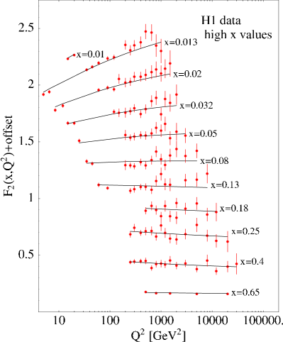
The determination of the different partons in given kinematic ranges can be split into a few different classes. We begin with large $\bf x$. Here the quark distributions are determined mainly from structure functions, which are dominated by non-singlet valence distributions. Both the evolution of these non-singlet distributions and conversion to structure functions is quite simple involving no parton mixing

$$\frac{df^{NS}(x,Q^{2})}{d\ln Q^{2}} = P^{NS}(x,\alpha_{s}(Q^{2}))\otimes f^{NS}(x,Q^{2})$$

$$F_{2}^{NS}(x,Q^{2}) = C^{NS}(x,\alpha_{s}(Q^{2}))\otimes f^{NS}(x,Q^{2}).$$

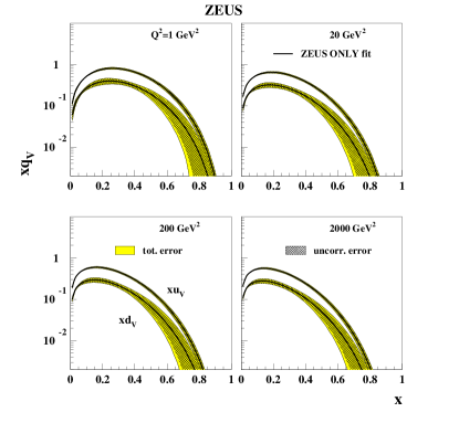
Hence, the evolution of high $x$ structure functions is a good test of the theory and of $\alpha_{S}(Q^{2})$. The success is shown in Fig. 1. However - perturbation theory involves contributions to the coefficient functions $\sim\alpha_{S}^{n}(Q^{2})\ln^{2n-1}(1-x)$ and higher twist contributions are known to be enhanced as $x\to 1$. Hence, in order to to avoid contamination of NLO theory one makes a cut $W^{2}=Q^{2}(1/x-1)+m_{p}^{2}\leq 10-15{\rm GeV}^{2}.$

figure=fig-BCDMS.ps,width=7.5truecm

Figure 1: Description of large $x$ BCDMS and SLAC measurements of $F_{2}^{p}$.

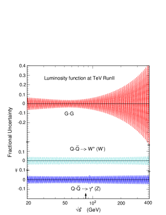
The extension to very small $\bf x$ has been made in the past decade by HERA. In this region there is very great scaling violation of the partons from the evolution equations and also interplay between the quarks and gluons. At each subsequent order in $\alpha_{S}$ each splitting function and coefficient function obtains an extra power of $\ln(1/x)$ (some accidental zeros in $P_{gg}$), i.e. $P_{ij}(x,\alpha_{s}(Q^{2})),C^{P}_{i}(x,\alpha_{s}(Q^{2}))\sim\alpha_{s}^{m}(Q^{2})\ln^{m-1}(1/x),$ and hence the convergence at small $x$ is questionable. The global fits usually assume that this turns out to be unimportant in practice, and proceed regardless. The fit is good, but could be improved. The large $\ln(1/x)$ terms mean that small $x$ predictions are somewhat uncertain, as will be discussed later. Small $x$ parton distributions are therefore an interesting field of study within QCD. They are also vital for understanding the standard production processes at the LHC, and perhaps some of the more exotic ones, as shown in Fig. 2, which demonstrates the range of $x$ probed by the experiment.

figure=LHCkin.ps,width=7.5truecm

Figure 2: The range of $x$ probed at HERA and the LHC as a function of the hard scale, e.g. particle mass, and rapidity.

figure=e866dis.ps,width=8.0truecm

Figure 3: E866 fit to their Drell-Yan data as a function of $x_{1}$ (quark) and $x_{2}$ (antiquark).

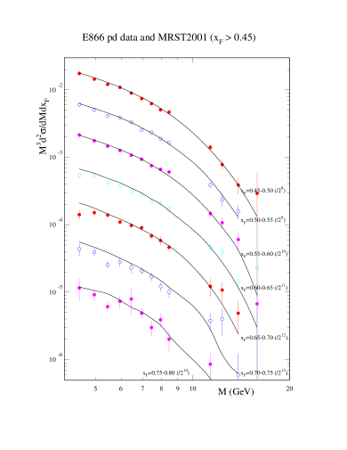
The high-$\bf x$ sea quarks are determined by Drell-Yan data (assuming good knowledge of the valence quarks). There is new precise data from the E866/NuSea collaboration[23], and their fit to these data shows a discrepancy with existing partons implying larger high-$x$ valence quarks, as shown in Fig. 4. However, the fit performed by MRST (Fig. 4) and CTEQ displays no such discrepancy.

Figure 4: MRST fit to the E866 data for high values of $x_{F}$.

The $\bf s(x)$ and $\bf\bar{s}(x)$ distributions are probed using CCFR and NuTeV dimuon data, i.e. the processes

$$\nu+s\to\mu^{-}+c(\mu^{+}),\quad\bar{\nu}+\bar{s}\to\mu^{+}+\bar{c}(\mu^{-}).$$

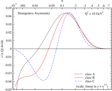
The quality of data is now such that one can examine the $s(x)$ and $\bar{s}(x)$ distributions separately. This has recently been performed in detail by CTEQ[24]. They find that $s(x)<\bar{s}(x)$ at quite small $x$, but since $\int(s(x)-\bar{s}(x))\,dx=0$, (zero strangeness number) this leads to $\to\int x(s(x)-\bar{s}(x))\,dx=[S^{-}]>0$, as demonstrated in Fig. 5. They obtain the rough constraint $0<[S^{-}]<0.004$. This is particularly significant because $NuTeV$ measure[25]

$$R^{-}=\frac{\sigma^{\nu}_{\rm NC}-\sigma^{\bar{\nu}}_{\rm NC}}{\sigma^{\nu}_{\rm CC}-\sigma^{\bar{\nu}}_{\rm CC}},$$

and in the standard model this satisfies $R^{-}=\frac{1}{2}-\sin^{2}\theta_{W}-(1-\frac{7}{3}\sin^{2}\theta_{W})\frac{[S^{-}]}{[V^{-}]}$. There is currently a $3\sigma$ discrepancy between this determination of $\sin^{2}\theta_{W}$ and others[26] but $[S^{-}]=0.002$ reduces this anomaly from $3\sigma$ to $1.5\sigma$. NuTeV themselves claim no such strange asymmetry when using partons obtained from fitting their own data[22], so this is an issue which requires resolution.

Figure 5: CTEQ strange momentum asymmetry (top) and number asymmetry (bottom).

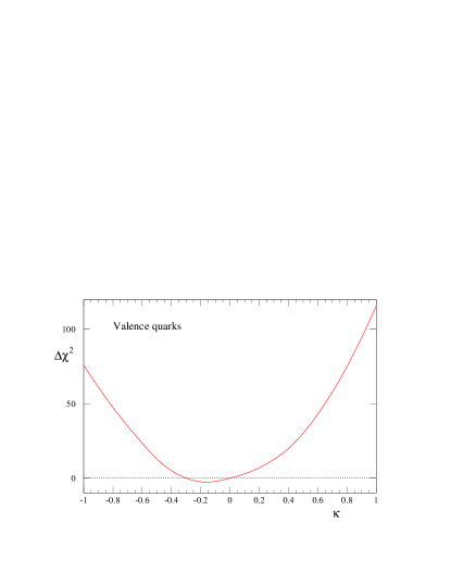
MRST also look at the effect of isospin violation[27] since $R^{-}$ also depends on this –

$$R^{-}=\frac{1}{2}-\sin^{2}\theta_{W}+(1-\frac{7}{3}\sin^{2}\theta_{W})\frac{[\delta U_{\rm v}]-[\delta D_{\rm v}]}{2[V^{-}]},$$

where $[\delta U_{\rm v}]=[U^{p}_{\rm v}]-[D^{n}_{\rm v}],$ $[\delta D_{\rm v}]=[D^{p}_{\rm v}]-[U^{n}_{\rm v}],$ and MRST use the simple parameterization

$$u^{p}_{\rm v}(x)=d^{n}_{\rm v}(x)+\kappa f(x),\qquad d^{p}_{\rm v}(x)=u^{n}_{\rm v}(x)-\kappa f(x),$$

where $f(x)$ is a simple function maintaining required conservation laws. The dependence on $\kappa$ is shown in Fig. 6. The best fit value of $\kappa=-0.2$ leads to a similar reduction of the NuTeV anomaly, i.e. $\Delta sin^{2}\theta_{W}\sim-0.002$. But there is only a weak indication of this value and a fairly wide variation in $\kappa$ is allowed.

Figure 6: $\Delta\chi^{2}$ against the isospin violating parameter $\kappa$.

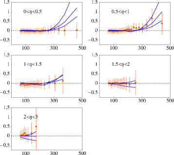
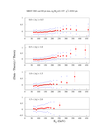
The best determination of the high-$\bf x$ gluon distribution comes from inclusive jet measurements by D0 and CDF at Tevatron. They measure $d\sigma/dE_{T}d\eta$ for central rapidity CDF or in bins of rapidity D0. At central rapidity the kinematic equality (at LO) is $x=2E_{T}/\sqrt{s}$, and measurements extend up to $E_{T}\sim 400{\rm GeV}\,(x\sim 0.45)$, and down to $E_{T}\sim 60{\rm GeV}\,(x\sim 0.06)$. Gluon-gluon fusion dominates the hard cross-section, but $g(x,\mu^{2})$ falls off more quickly as $x\to 1$ than $q(x,\mu^{2})$ so there is a transition from gluon-gluon fusion at small $x$, to gluon-quark to quark-quark at high $x$. However, as seen in Fig. 7 even at the highest $x$ gluon-quark contributions are significant. Jet photoproduction at HERA will be another constraint in the future.

Figure 7: Fractional contributions to jet cross-section from different parton-level contributions.

The above procedure completely determines the parton distributions at present. The total fit is reasonably good and that for CTEQ6[2] is shown in Table 1 for the large data sets. The total $\chi^{2}=1954/1811$. For MRST The total $\chi^{2}=2328/2097$ – but the errors are treated differently, and different data sets and cuts are used. The same sort of conclusion is true for other global fits[3]^-[7] (which use fewer data). However, there are some areas where the theory perhaps needs to be improved, as we will discuss later.

Table 1: Quality of fit to data for CTEQ6M.

Data Set	no. of data	$\chi^{2}$
H1 $ep$	230	228
ZEUS $ep$	229	263
BCDMS $\mu p$	339	378
BCDMS $\mu d$	251	280
NMC $\mu p$	201	305
E605 (Drell-Yan)	119	95
D0 Jets	90	65
CDF Jets	33	49

2 Parton Uncertainties

2.1 Hessian (Error Matrix) approach

In this one defines the Hessian matrix $H$ by

$$\chi^{2}-\chi_{min}^{2}\equiv\Delta\chi^{2}=\sum_{i,j}H_{ij}(a_{i}-a_{i}^{(0)})(a_{j}-a_{j}^{(0)}).$$

$H$ is related to the covariance matrix of the parameters by $C_{ij}(a)=\Delta\chi^{2}(H^{-1})_{ij},$ and one can use the standard formula for linear error propagation,

$$(\Delta F)^{2}=\Delta\chi^{2}\sum_{i,j}\frac{\partial F}{\partial a_{i}}(H)^{-1}_{ij}\frac{\partial F}{\partial a_{j}}.$$

This has been employed to find partons with errors by Alekhin[5], as seen in Fig. 8 and H1[6] (each with restricted data sets).

Figure 8: Results for Alekhin partons at $Q^{2}=9\,{\rm GeV}^{2}$ with uncertainties (solid lines), (dashed lines – CTEQ5M, dotted lines – MRST01).

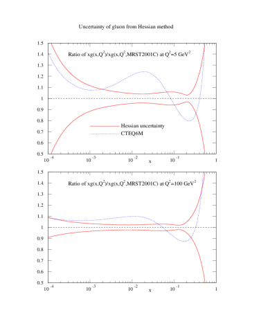
The simple method can be problematic with larger data sets and larger numbers of parameters due to extreme variations in $\Delta\chi^{2}$ in different directions in parameter space. This is solved by finding and rescaling the eigenvectors of $H$ (CTEQ[28, 29, 2]) leading to the diagonal form

$$\Delta\chi^{2}=\sum_{i}z_{i}^{2}.$$

The uncertainty on a physical quantity is given by

$$(\Delta F)^{2}=\sum_{i}\bigl{(}F(S_{i}^{(+)})-F(S_{i}^{(-)})\bigr{)}^{2},$$

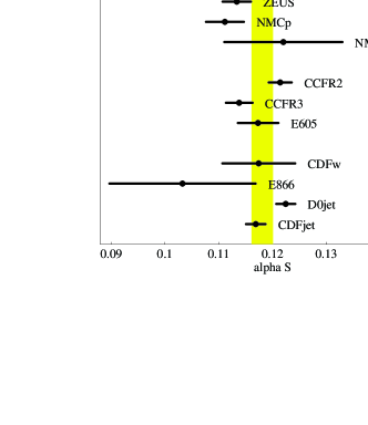
where $S_{i}^{(+)}$ and $S_{i}^{(-)}$ are PDF sets displaced along eigenvector directions by a given $\Delta\chi^{2}$. Similar eigenvector parton sets have also been introduced by MRST[31] and ZEUS. However, there is an art in choosing the “correct” $\Delta\chi^{2}$ given the complication of the errors in the full fit[32]. Ideally $\Delta\chi^{2}=1$, but this leads to unrealistic errors, e.g. values of $\alpha_{S}(M_{Z}^{2})$ obtained by CTEQ using $\Delta\chi^{2}=1$ for each data set in the global fit are shown in Fig. 9, and are not consistent. CTEQ choose $\Delta\chi^{2}\sim 100$, which is perhaps conservative. MRST choose $\Delta\chi^{2}\sim 50$. An example of results is shown in Fig. 10.

Figure 9: Values of $\alpha_{S}(M_{Z}^{2})$ and their uncertainties using $\Delta\chi^{2}=1$ from CTEQ.

Figure 10: Luminosity uncertainties using the CTEQ Hessian approach.

2.2 Offset method

In this the best fit and parameters $a_{0}$ are obtained using only uncorrelated errors. The quality of the fit is then estimated by adding uncorrelated and correlated errors in quadrature. Roughly speaking systematic uncertainties are determined by letting each source of systematic error vary by $1\sigma$ and adding the deviations in quadrature. This procedure is used by ZEUS[7], and leads to an effective $\Delta\chi^{2}>1$.

Figure 11: The valence partons extracted by ZEUS from a global fit and a fit to their own data alone (with some input assumptions). The latter illustrates a potential for a real constraint from HERA data alone in the future.

2.3 Statistical Approach

In principle this involves the construction of an ensemble of distributions labelled by ${\cal F}$ each with probability $P(\{{\cal F}\})$, where one can incorporate the full information about measurements and their error correlations into the calculation of $P(\{{\cal F}\})$. This is statistically correct, and does not rely on the approximation of linear propagation errors in calculating observables. However, it is inefficient, and in practice one generates $N$ ($N$ can be as low as $100$) different distributions with unit weight but distributed according to $P(\{{\cal F}\})$[4]. Then the mean $\mu_{O}$ and deviation $\sigma_{O}$ of an observable $O$ are given by

$$\mu_{O}=\frac{1}{N}\sum_{1}^{N}O(\{{\cal F}\}),\,\sigma_{O}^{2}=\frac{1}{N}\sum_{1}^{N}(O(\{{\cal F}\})-\mu_{O})^{2}.$$

Currently this approach uses only proton DIS data sets in order to avoid complicated uncertainty issues, e.g. shadowing effects for nuclear targets, and also demands consistency between data sets. However, it is difficult to find many truly compatible DIS experiments, and consequently the Fermi2001 partons are determined by only H1, BCDMS, and E665 data sets. They result in good predictions for many Tevatron cross-sections, e.g. inclusive jets and $W$ and $Z$ total cross-sections. However, the restricted data sets mean there is restricted information – data sets are deemed either perfect or, in the case of most of them, useless – leading to unusual values for some parameters. e.g. $\alpha_{S}(M_{Z}^{2})=0.112\pm 0.001$ and a very hard $d_{V}(x)$ at high $x$ (together these two features facilitate a good fit to Tevatron jets independent of the high-$x$ gluon). These partons would produce some extreme predictions, as seen later. Nevertheless, the approach does demonstrate that the Gaussian approximation is often not good, and therefore highlights shortcomings in the methods outlined in the previous sections. It is a very attractive, but ambitious large-scale project, still in need of some further development. In particular I feel it requires the inclusion of a wider variety of data in order to overcome the obstacle presented by the fact that most data sets in the global fit are not really as consistent as they should be in the strict statistical sense.

2.4 Lagrange Multiplier method

This was first suggested by CTEQ[30] and has been concentrated on by MRST[31]. One performs the fit while constraining the value of some physical quantity, i.e. one minimizes

$$\Psi(\lambda,a)=\chi^{2}_{global}(a)+\lambda F(a)$$

for various values of $\lambda$. This gives a set of best fits for particular values of the quantity $F(a)$ without relying on the quadratic approximation for $\chi^{2}$, as shown for $\sigma_{W}$ in Fig. 12. The uncertainty is then determined by deciding an allowed range of $\Delta\chi^{2}$. One can also easily check the variation in $\chi^{2}$ for each of the experiments in the global fit and ascertain if the total $\Delta\chi^{2}$ is coming specifically from one region, which might cause concern. In principle, this is superior to the Hessian approach, but it must be repeated for each physical process.

Figure 12: $\chi^{2}_{global}$ for CTEQ plotted against $\sigma_{W}$.

2.5 Results

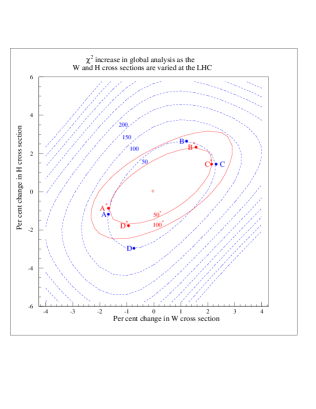
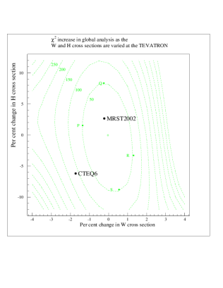
I choose the cross-section for $W$ and Higgs production at the Tevatron and LHC (for $M_{H}=115{\rm GeV}$) as examples. Using their fixed value of $\alpha_{S}(M_{Z}^{2})=0.118$ and $\Delta\chi^{2}=100$ CTEQ obtain

$$\Delta\sigma_{W}(\rm LHC)\approx\pm 4\%\quad\Delta\sigma_{W}({\rm Tev})\approx\pm 5\%$$

$$\Delta\sigma_{H}({\rm LHC})\approx\pm 5\%.$$

Using a slightly wider range of data, $\Delta\chi^{2}\sim 50$ and $\alpha_{S}(M_{Z}^{2})=0.119$ MRST obtain

$$\Delta\sigma_{W}(\rm Tev)\approx\pm 1.2\%\quad\Delta\sigma_{W}({\rm LHC})\approx\pm 2\%$$

$$\Delta\sigma_{H}(\rm Tev)\approx\pm 4\%\quad\Delta\sigma_{H}({\rm LHC})\approx\pm 2\%.$$

MRST also allow $\alpha_{S}(M_{Z}^{2})$ to be free. In this case $\Delta\sigma_{W}$ is quite stable but $\Delta\sigma_{H}$ almost doubles. Contours of variation in $\chi^{2}$ for the predictions of these cross-sections are shown in Fig. 13.

Figure 13: $\chi^{2}$-plot for $W$ and Higgs production at the Tevatron (top) and LHC (bottom) with $\alpha_{S}$ free (dashed) and fixed (solid) at $\alpha_{S}=0.119$

The same general procedure is also used by CTEQ[34] to look at the effect of new physics parameterized by the contact term

$$\pm(2\pi/\Lambda^{2})(\bar{q}_{L}\gamma^{\mu}q_{L})(\bar{q}_{L}\gamma_{\mu}q_{L}).$$

The curves in Fig. 14 show the fit to the $D0$ jet data, which is the most discriminating data set, for $\Lambda=1.6,2.0,2.4,\infty\,\,\hbox{\rm TeV}$, and $A=-1$. For the highest values of $\Lambda$ the fit even improves very slightly, but $\Lambda>1.6,\,\hbox{\rm TeV}$ is clearly ruled out.

Figure 14: Fits to D0 jets for different values of $A$.

Table 2: Values of $\alpha_{s}(M_{Z}^{2})$ and its error from different NLO QCD fits.

Group	$\Delta\chi^{2}$	$\alpha_{S}(M_{Z}^{2})$
CTEQ6	$\Delta\chi^{2}=100$	$\alpha_{s}(M_{Z}^{2})=$	$0.1165\pm 0.0065(exp)$
ZEUS	$\Delta\chi_{eff}^{2}=50$	$\alpha_{s}(M_{Z}^{2})=$	$0.1166\pm 0.0049(exp)$ $\pm 0.0018(model)$ $\pm 0.004(theory)$
MRST01	$\Delta\chi^{2}=20$	$\alpha_{s}(M_{Z}^{2})=$	$0.1190\pm 0.002(exp)$ $\pm 0.003(theory)$
H1	$\Delta\chi^{2}=1$	$\alpha_{s}(M_{Z}^{2})=$	$0.115\pm 0.0017(exp)$ ${}^{+~{}~{}0.0009}_{-~{}~{}0.0005}~{}(model)$ $\pm 0.005(theory)$
Alekhin	$\Delta\chi^{2}=1$	$\alpha_{s}(M_{Z}^{2})=$	$0.1171\pm 0.0015(exp)$ $\pm 0.0033(theory)$
GKK	CL	$\alpha_{s}(M_{Z}^{2})=$	$0.112\pm 0.001(exp)$

Hence, the estimation of uncertainties due to experimental errors has many different approaches and different types and amount of data actually fit. Overall the uncertainty from this source is rather small – only more than a few $\%$ for quantities determined by the high $x$ gluon and very high $x$ down quark. This is illustrated for the determinations of $\alpha_{S}(M_{Z}^{2})$ in Table 2. There is generally good agreement, but their are some outlying values.

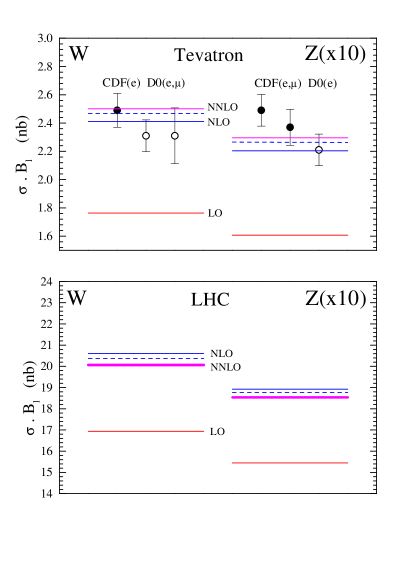
These outlying values of $\alpha_{S}(M_{Z}^{2})$ show that different approaches can sometimes lead to rather different central values, This suggests that there are other matters to consider as well as the experimental errors on data. We also need to determine the effect of assumptions made about the fit, e.g. cuts made on the data, the data sets fit, the parameterization for input sets, the form of the strange sea, etc.. Many of these can be as important as the errors on the data used (or more so). This is demonstrated by the results from the LHC/LP Study Working Group[35] shown in Tables 3, and by predictions for $\sigma_{W}$ by MRST CTEQ and Alekhin[36] in Table 4. In both cases the discrepancies are mainly due to differences in detailed constraints (by data) on the quark decomposition. Differences between predictions are also shown by Fig. 15 – the predictions for $W$ and Higgs production at the Tevatron from MRST2001 and CTEQ6, and Fig. 16 – the comparison between the gluons for the two parton sets.

Table 3: Cross sections for Drell-Yan pairs ($e^{+}e^{-}$) with PYTHIA 6.206, rapidity $<2.5$. The errors shown are the PDF uncertainties.

PDF set	Comment	xsec [pb]	PDF uncertainty %
$81<M<101$ GeV
CTEQ6	LHAPDF	1065 $\pm$ 46	4.4
MRST2001	LHAPDF	1091 $\pm$ …	3
Fermi2002	LHAPDF	853 $\pm$ 18	2.2

Table 4: Comparison of $\sigma_{W}\cdot B_{l\nu}$ for different partons.

PDF set	Comment	xsec [nb]	PDF uncertainty
Alekhin	Tevatron	2.73	$\pm$ 0.05 (tot)
MRST2002	Tevatron	2.59	$\pm$ 0.03 (expt)
CTEQ6	Tevatron	2.54	$\pm$ 0.10 (expt)
Alekhin	LHC	215	$\pm$ 6 (tot)
MRST2002	LHC	204	$\pm$ 4 (expt)
CTEQ6	LHC	205	$\pm$ 8 (expt)

Figure 15: $\chi^{2}$-plot for $W$ and Higgs production at the Tevatron with $\alpha_{S}$ free. The predictions from CTEQ6 is marked.

Figure 16: Fractional uncertainty in the MRST gluon compared with the difference in the central CTEQ6 gluon.

3 Theoretical errors

3.1 Problems in the fit

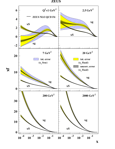
As well as the consequences of these assumptions we must consider the related problem of theoretical errors. Theoretical errors are indicated by some regions where the theory perhaps needs to be improved to fit the data better. There is a reasonably good fit to HERA data, but there are some problems at the highest $Q^{2}$ at moderate $x$, i.e. in $dF_{2}/d\ln Q^{2}$, as seen for MRST and CTEQ in Fig. 17. Also the data require the gluon to be valencelike or negative at small $x$ at low $Q^{2}$, e.g. the ZEUS gluon in Fig. 18, leading to $F_{L}(x,Q^{2})$ being negative[1] at the smallest $x,Q^{2}$. However, it is not just the low $x$–low $Q^{2}$ data that require this negative gluon. The moderate $x$ data need lots of gluon to get a reasonable $dF_{2}/d\ln Q^{2}$ and the Tevatron jets need a large high $x$ gluon, and this must be compensated for elsewhere. In general MRST find that it is difficult to reconcile the fit to jets and to the rest of the data, Fig. 19, and that different data compete over the gluon and $\alpha_{S}(M_{Z}^{2})$. The jet fit is better for CTEQ6 largely due to their different cuts on other data. Other fits do not include the Tevatron jets, but generally produce gluons largely incompatible with this data.

Figure 17: Comparison of MRST(2001) $F_{2}(x,Q^{2})$ with HERA, NMC and E665 data (top) and CTEQ6 $F_{2}(x,Q^{2})$ with H1 data (bottom).

Figure 18: Zeus gluon and sea quark distributions at various $Q^{2}$ values.

Figure 19: The MRST fit to D0 jet data. The points show the range of the systematic errors.

3.2 Types of Theoretical Error, NNLO

It is vital to consider theoretical errors. These include higher perturbative orders (NNLO), small $x$ ($\alpha_{s}^{n}\ln^{n-1}(1/x)$), large $x$ ($\alpha_{s}^{n}\ln^{2n-1}(1-x)$) low $Q^{2}$ (higher twist), etc.. Note that renormalization/factorization scale variation is not a reliable method of estimating these theoretical errors because of increasing logs at higher orders.

Figure 20: LO, NLO and NNLO predictions for $W$ and $Z$ cross-sections.

In order to investigate the true theoretical error we must consider some way of performing correct large and small $x$ resummations, and/or use what we already know about NNLO. The coefficient functions are known at NNLO. Singular limits $x\to 1$, $x\to 0$ are known for NNLO splitting functions as well as limited moments[37], and this has allowed approximate NNLO splitting functions to be devised[38] which have been used in approximate global fits[39]. They improve the quality of fit very slightly (mainly at high $x$) and $\alpha_{S}(M_{Z}^{2})$ lowers from $0.119$ to 0.1155. The gluon is smaller at NNLO at low $x$ due to the positive NNLO quark-gluon splitting function. There is also a NNLO fit by Alekhin[40], with some differences – the gluon is not smaller, probably due to the absence of Tevatron jet data in the fit and to a very different definition of the NNLO charm contribution. There is agreement in the reduction of $\alpha_{S}(M_{Z}^{2})$ at NNLO, i.e. $0.1171\to 0.1143$.

Using these NNLO partons there is reasonable stability order by order for the (quark-dominated) $W$ and $Z$ cross-sections, as seen in Fig. 20. However, the change from NLO to NNLO is of order $4\%$, which is much bigger than the uncertainty at NLO due to experimental errors. Also, this fairly good convergence is largely guaranteed because the quarks are fit directly to data. There is greater danger in gluon dominated quantities, e.g. $F_{L}(x,Q^{2})$, as can be seen in Fig. 21. Hence, the convergence from order to order is uncertain.

Figure 21: Comparison of the predictions for $F_{L}(x,Q^{2})$ at LO, NLO and NNLO using MRST partons and also a $\ln(1/x)$-resummed prediction[42].

3.3 Empirical approach

We can estimate where theoretical errors may be important by adopting the empirical approach of investigating in detail the effect of cuts on the fit quality, i.e. we try varying the kinematic cuts on data. The procedure is to change $W^{2}_{cut}$, $Q^{2}_{cut}$ and/or $x_{cut}$, re-fit and see if the quality of the fit to the remaining data improves and/or the input parameters change dramatically. (This is similar to a previous suggestion in terms of data sets[41].) One then continues until the quality of the fit and the partons stabilize[27].

For $W^{2}_{cut}$ raising from $15{\rm GeV}^{2}$ has no effect. When raising $Q^{2}_{cut}$ from $2{\rm GeV}^{2}$ in steps there is a slow, continuous and significant improvement for $Q^{2}$ up to $>10{\rm GeV}^{2}$ (560 data points cut), suggesting that any corrections are probably higher orders not higher twist. The input gluon becomes slightly smaller at low $x$ at each step (where one loses some of the lowest $x$ data), and larger at high $x$. $\alpha_{S}(M_{Z}^{2})$ slowly decreases by about 0.0015. Raising $x_{cut}$ leads to continuous improvement with stability reached at $x=0.005$ (271 data points cut) with $\alpha_{S}(M_{Z}^{2})\to 0.118$. There is an improvement in the fit to HERA, NMC and Tevatron jet data, and much reduced tension between the data sets. At each step the moderate $x$ gluon becomes more positive, at the expense of the gluon below the cut becoming very negative and $dF_{2}(x,Q^{2})/d\ln Q^{2}$ being incorrect. However, higher orders could cure this in a quite plausible manner. For example adding higher order terms to the splitting functions

$$P_{gg}\to....+\frac{3.86\bar{\alpha}_{S}^{4}}{x}\biggr{(}\frac{\ln^{3}(1/x)}{6}-\frac{\ln^{2}(1/x)}{2}\biggr{)},$$

$$P_{qg}\to....+\frac{5.12N_{f}\bar{\alpha}_{S}^{5}}{6x}\biggr{(}\frac{\ln^{3}(1/x)}{6}-\frac{\ln^{2}(1/x)}{2}\biggr{)},$$

leaves the improved fit above $x=0.005$ largely unchanged, but solves the problem below $x=0.005$. Saturation corrections added to NLO and NNLO fits seem to make the situation worse. Hence, the cuts are suggestive of theoretical errors for small $x$ and/or small $Q^{2}$. Predictions for $W$ and Higgs cross-sections at the Tevatron are still safe if $x_{cut}=0.005$, since they do not sample partons at lower $x$. However, they change in a smooth manner as $x_{cut}$ is lowered, due to the altered partons above $x_{cut}$.

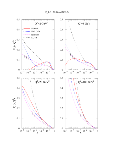
There is a lot of work on explicit $\ln(1/x)$-resummations in structure functions and parton distributions for example[42, 43, 44], but there is no complete consensus on the best approach. There is also work on connecting the partons to alternative approaches at small $x$, e.g. dipole models[45], and pomerons[46]. These approaches can suggest improvements to the fits and changes in predictions, e.g. a resummed prediction[42] for $F_{L}(x,Q^{2})$ is shown on Fig. 21. Accurate and direct measurements of $F_{L}(x,Q^{2})$ and other quantities at low $x$ and/or $Q^{2}$ (the predicted range and accuracy of $F_{L}(x,Q^{2})$ measurements at HERA III is shown on Fig. 21) would be a great help in determining whether $NNLO$ is sufficient or whether resummed (or other) corrections are necessary, or helpful for maximum precision.

4 Conclusions

One can perform global fits to all up-to-date data over a wide range of parameter space, and there are various ways of looking at uncertainties due to errors on data alone. There is no totally preferred approach. The errors from this source are rather small – $\sim 1-5\%$ except in a few regions of parameter space and are similar using various approaches. The uncertainty from input assumptions e.g. cuts on data, parameterizations etc., are comparable and sometimes larger, which means one cannot entirely believe one group’s errors.

The quality of the fit is fairly good, but there are some slight problems. These imply that errors from higher orders/resummation are potentially large in some regions of parameter space, and due to correlations between partons these affect all regions (the small $x$ gluon influences the large $x$ gluon). Cutting out low $x$ and/or $Q^{2}$ data allows a much-improved fit to the remaining data, and altered partons. Hence, for some processes theory is probably the dominant source of uncertainty at present and a systematic study is a priority as is more data which would help determine our theoretical accuracy.

References

- [1] A.D. Martin et al., Eur. Phys. J. C23 73 (2002).
- [2] CTEQ Collaboration: J. Pumplin et al., JHEP 0207:012 (2002).
- [3] M. Botje, Eur. Phys. J. C14 285 (2000).
- [4] W.T. Giele and S. Keller, Phys. Rev. D58 094023 (1998); W.T. Giele, S. Keller and D.A. Kosower, hep-ph/0104052.
- [5] S.I. Alekhin, Phys. Rev. D68 014002 (2003).
- [6] H1 Collaboration: C. Adloff et al., Eur. Phys. J. C21 33 (2001).
- [7] A.M. Cooper-Sarkar, J. Phys. G28 2669 (2002); ZEUS Collaboration: S. Chekanov et al., Phys. Rev. D67 012007 (2003).
- [8] H1 Collaboration: C. Adloff et al., Eur. Phys. J. C13 609 (2000); H1 Collaboration: C. Adloff et al., Eur. Phys. J. C19 269 (2001).
- [9] ZEUS Collaboration: S. Chekanov et al., Eur. Phys. J. C21 443 (2001); ZEUS Collaboration: S. Chekanov et al., Eur. Phys. J. C28 175 (2003).
- [10] M.R. Adams et al., Phys. Rev. D54 3006 (1996).
- [11] BCDMS Collaboration: A.C. Benvenuti et al., Phys. Lett. B223 485 (1989); BCDMS Collaboration: A.C. Benvenuti et al., Phys. Lett. B236 592 (1989).
- [12] L.W. Whitlow et al., Phys. Lett. B282 475 (1992), L.W. Whitlow, preprint SLAC-357 (1990).
- [13] NMC Collaboration: M. Arneodo et al., Nucl. Phys. B483 3 (1997); Nucl. Phys. B487 3 (1997).
- [14] CCFR Collaboration: U.K. Yang et al., Phys. Rev. Lett. 86 2742 (2001); CCFR Collaboration: W.G. Seligman et al., Phys. Rev. Lett. 79 1213 (1997).
- [15] ZEUS Collaboration: J. Breitweg et al., Eur. Phys. J. C12 35 (2000).
- [16] H1 Collaboration: C. Adloff et al., Phys. Lett. B528 1999 (2002).
- [17] E605 Collaboration: G. Moreno et al., Phys. Rev. D43 2815 (1991).
- [18] E866 Collaboration: R.S. Towell et al., Phys. Rev. D64 052002 (2001).
- [19] CDF Collaboration: F. Abe et al., Phys. Rev. Lett. 81 5744 (1998).
- [20] D0 Collaboration: B. Abbott et al., Phys. Rev. Lett. 86 1707 (2001).
- [21] CDF Collaboration: T. Affolder et al., Phys. Rev. D64 032001 (2001).
- [22] NuTeV Collaboration: M. Goncharov et al., Phys. Rev. D64 112006 (2001).
- [23] E866/NuSea Collaboration: J.C. Webb et al, hep-ex/0302019.
- [24] S. Kretzer et al, preprint BNL-NT-03/16.
- [25] NuTeV Collaboration: G.P. Zeller et al, Phys. Rev. Lett. 88 091802 (2002).
- [26] P. Gambino, these proceedings.
- [27] A.D. Martin, R.G. Roberts, W.J. Stirling and R.S. Thorne, hep-ph/0308087, submitted to Eur. Phys. J.
- [28] CTEQ Collaboration: J. Pumplin et al., Phys. Rev. D65 014011 (2002).
- [29] CTEQ Collaboration: J. Pumplin et al., Phys. Rev. D65 014013 (2002).
- [30] CTEQ Collaboration: D. Stump et al., Phys. Rev. D65 014012 (2002).
- [31] A.D.Martin et al Eur. Phys. J. C28 455 (2003).
- [32] R.S. Thorne et al., J. Phys. G28 2717 (2002).
- [33] C. Pascaud and F. Zomer 1995 Preprint LAL-95-05.
- [34] D. Stump et al, hep-ph/0303013.
- [35] D. Bourilkov, hep-ph/0305125.
- [36] S. Alekhin, hep-ph0307219.
- [37] S.A. Larin et al., Nucl. Phys. B492 338 (1997); A. Rétey and J.A.M. Vermaseren, Nucl. Phys. B604 281 (2001).
- [38] W.L. van Neerven and A. Vogt, Phys. Lett. B490 111 (2000).
- [39] A.D. Martin et al., Phys. Lett. B531 216 (2002).
- [40] S.I. Alekhin, Phys. Lett. B519 57 (2001).
- [41] J. C. Collins and J. Pumplin, hep-ph/0105207.
- [42] R.S. Thorne, Phys. Rev. D64 074005 (2001).
- [43] M. Ciafaloni, et al, hep-ph/0307188.
- [44] G. Altarelli, et al, hep-ph/0306156.
- [45] J. Bartels, et al, Phys. Rev. D66 014001 (2002).
- [46] A. Donnachie and P.V. Landshoff, Phys. Lett. B550 160 (2002).