The Gluon Green’s Function in the BFKL Approach at Next–to–Leading Logarithmic Accuracy

Abstract

We investigate the gluon Green’s function in the high energy limit of QCD using a recently proposed iterative solution of the Balitsky–Fadin–Kuraev–Lipatov (BFKL) equation at next–to–leading logarithmic (NLL) accuracy. To establish the applicability of this method in the NLL approximation we solve the BFKL equation as originally written by Fadin and Lipatov, and compare the results with previous studies in the leading logarithmic (LL) approximation.

,

1 Introduction

The Balitsky–Fadin–Kuraev–Lipatov [1] formalism resums a class of logarithms dominant in the Regge limit of scattering amplitudes where the centre of mass energy $\sqrt{s}$ is large and the momentum transfer $\sqrt{-t}$ is fixed. Within this approach the high energy cross–section for the process $A+B\rightarrow A^{\prime}+B^{\prime}$ can be written as

$$\sigma(s) = \int\frac{d^{2}{\bf k}_{a}}{2\pi{\bf k}_{a}^{2}}\int\frac{d^{2}{\bf k}_{b}}{2\pi{\bf k}_{b}^{2}}~{}\Phi_{A}({\bf k}_{a})~{}\Phi_{B}({\bf k}_{b})~{}f\left({\bf k}_{a},{\bf k}_{b},\Delta\equiv\ln{\frac{s}{s_{0}}}\right),$$ (1)

with $\Phi_{A,B}$ being the process–dependent impact factors and $f\left({\bf k}_{a},{\bf k}_{b},\Delta\right)$ the process–independent gluon Green’s function. This gluon Green’s function describes the interaction between two Reggeised gluons exchanged in the $t$–channel with transverse momenta ${\bf k}_{a,b}$, and it carries the energy dependence of the cross–section. We choose to work with the symmetric Regge scale $s_{0}=k_{a}k_{b}$, where $k_{i}\equiv\left|{\bf k}_{i}\right|$.

The resummation of terms of the form $\left(\alpha_{s}\Delta\right)^{n}$ defines the LL accuracy while the inclusion of contributions proportional to $\alpha_{s}\left(\alpha_{s}\Delta\right)^{n}$ leads to the NLL approximation. The ladder structure of the scattering amplitudes derived in the BFKL formalism is described by an integral equation for the gluon Green’s function. The eigenfunctions of this integral equation are known at LL accuracy and it is therefore possible to fully reconstruct the solution. One of the motivations to include the NLL contributions is to introduce running coupling effects. The logarithmic dependence introduced by the running coupling terms in the NLL approximation significantly complicates the study of the equation [2]. During the past few years different strategies have been suggested to study the NLL BFKL Green’s function. In a fixed coupling analysis in Ref. [3] it was first highlighted that the NLL corrections are large and negative compared to the LL. Different approaches to improve the convergence of the series expansion at NLL accuracy have been proposed [4]. When running coupling effects are taken into account the situation improves as it has been shown in Ref. [5], in particular when those terms proportional to $\beta_{0}$ are resummed into $\alpha_{s}$.

Recently, we proposed [6] to use an iterative approach to solve the equation in the NLL approximation. A similar method was first suggested at the LL accuracy in Ref. [7], where it was shown to reproduce the analytic solution, and opened the possibility to perform detailed LL phenomenological studies [8].

The NLL formalism of Ref. [6] has the advantage of dealing with the BFKL kernel as calculated in Ref. [9, 10] with no approximations. In particular, the solution includes all running coupling effects and, as we do not use the angular averaged kernel, it allows for a complete study of angular dependences. The main purpose of this paper is to establish the applicability of the NLL solution put forward in Ref. [6]. With such intention we will solve the NLL BFKL equation as originally written in [9], with a particular choice of renormalisation scale. Running coupling effects therefore correspond to an expansion of the one–loop running of $\alpha_{s}(\mu)$ in the ${\overline{\rm MS}}$ scheme. A study of different schemes for the running of the coupling and choices for the renormalisation scale will be presented in a future publication.

This paper is organised as follows: In Section 2 we present the BFKL equation and sketch the derivation of the iterative solution following Ref. [6]. In Section 3 we present a numerical analysis of the NLL kernel, briefly indicating the mathematical expressions used in our numerical implementation. In Section 4 we use this numerical implementation to study the NLL gluon Green’s function. We analyse the convergence of the solution and its dependence on the transverse momenta of the gluons exchanged in the $t$–channel. We present results on the evolution of the gluon Green’s function and a study of the renormalisation scale dependence. We also show results on angular dependences and a toy cross section obtained using simplified LL impact factors, to finally present our conclusions in Section 5.

2 The Solution of the NLL BFKL Equation

In this Section we sketch the method of solution for the BFKL equation at NLL accuracy proposed in Ref. [6]. To write the equation in a convenient way we first perform a Mellin transform of the gluon Green’s function, i.e.

$$f\left({\bf k}_{a},{\bf k}_{b},\Delta\right)=\frac{1}{2\pi i}\int_{a-i\infty}^{a+i\infty}d\omega~{}e^{\omega\Delta}f_{\omega}\left({\bf k}_{a},{\bf k}_{b}\right).$$ (2)

With such a transformation the BFKL equation in dimensional regularisation $\left(D=4+2\epsilon\right)$ reads [9]

$$\omega f_{\omega}\left({\bf k}_{a},{\bf k}_{b}\right) = \delta^{(2+2\epsilon)}\left({\bf k}_{a}-{\bf k}_{b}\right)+\int d^{2+2\epsilon}{\bf k}^{\prime}~{}\mathcal{K}\left({\bf k}_{a},{\bf k}^{\prime}\right)f_{\omega}\left({\bf k}^{\prime},{\bf k}_{b}\right),$$ (3)

where the kernel is expressed in terms of the gluon Regge trajectory and the real emission component in the following way

$$\mathcal{K}\left({\bf k}_{a},{\bf k}\right)=2\,\omega^{(\epsilon)}\left({\bf k}_{a}^{2}\right)\,\delta^{(2+2\epsilon)}\left({\bf k}_{a}-{\bf k}\right)+\mathcal{K}^{(\epsilon)}_{r}\left({\bf k}_{a},{\bf k}\right)+{\tilde{\mathcal{K}}}_{r}\left({\bf k}_{a},{\bf k}\right).$$ (4)

Both $\epsilon$–dependent parts of the kernel contain $1/\epsilon$ and $1/\epsilon^{2}$ poles. The cancellation of the poles in the trajectory against those in the real emission kernel was shown in Ref. [6] by introducing a phase space slicing parameter $\lambda$. The BFKL equation can then be expressed as

$$\left(\omega-\omega_{0}\left({\bf k}_{a}^{2},\lambda^{2}\right)\right)f_{\omega}\left({\bf k}_{a},{\bf k}_{b}\right) = \delta^{(2)}\left({\bf k}_{a}-{\bf k}_{b}\right)$$

$$+\int d^{2}{\bf k}\left(\frac{1}{\pi{\bf k}^{2}}\xi\left({\bf k}^{2}\right)\theta\left({\bf k}^{2}-\lambda^{2}\right)+\widetilde{\mathcal{K}}_{r}\left({\bf k}_{a},{\bf k}_{a}+{\bf k}\right)\right)f_{\omega}\left({\bf k}_{a}+{\bf k},{\bf k}_{b}\right),$$

where $\widetilde{\mathcal{K}}_{r}$ is the finite part of the emission kernel,

$$\widetilde{\mathcal{K}}_{r}\left({\bf q},{\bf q}^{\prime}\right) = \frac{\bar{\alpha}_{s}^{2}(\mu)}{4\pi}\left\{\left(1+\frac{n_{f}}{N_{c}^{3}}\right)\frac{\left(3({\bf q}\cdot{\bf q^{\prime}})^{2}-2{\bf q}^{2}{\bf q^{\prime}}^{2}\right)}{16{\bf q}^{2}{\bf q^{\prime}}^{2}}\left(\frac{2}{{\bf q}^{2}}+\frac{2}{{\bf q^{\prime}}^{2}}\right.\right.$$ (6)

$$\left.+\left(\frac{1}{{\bf q^{\prime}}^{2}}-\frac{1}{{\bf q}^{2}}\right)\ln{\frac{{\bf q}^{2}}{{\bf q^{\prime}}^{2}}}\right)+\frac{2({\bf q}^{2}-{\bf q^{\prime}}^{2})}{({\bf q}-{\bf q^{\prime}})^{2}({\bf q}+{\bf q^{\prime}})^{2}}\left(\frac{1}{2}\ln{\frac{{\bf q}^{2}}{{\bf q^{\prime}}^{2}}}\ln{\frac{{\bf q}^{2}{\bf q^{\prime}}^{2}({\bf q}-{\bf q^{\prime}})^{4}}{({\bf q}^{2}+{\bf q^{\prime}}^{2})^{4}}}\right.$$

$$\left.+\left(\int_{0}^{-{\bf q}^{2}/{\bf q^{\prime}}^{2}}-\int_{0}^{-{\bf q^{\prime}}^{2}/{\bf q}^{2}}\right)dt\frac{\ln(1-t)}{t}\right)-\frac{1}{({\bf q}-{\bf q^{\prime}})^{2}}\ln^{2}{\frac{{\bf q}^{2}}{{\bf q^{\prime}}^{2}}}$$

$$-\left(3+\left(1+\frac{n_{f}}{N^{3}_{c}}\right)\left(1-\frac{({\bf q}^{2}+{\bf q^{\prime}}^{2})^{2}}{8{\bf q}^{2}{\bf q^{\prime}}^{2}}-\frac{(2{\bf q}^{2}{\bf q^{\prime}}^{2}-3{\bf q}^{4}-3{\bf q^{\prime}}^{4})}{16{\bf q}^{4}{\bf q^{\prime}}^{4}}({\bf q}\cdot{\bf q^{\prime}})^{2}\right)\right)$$

$$\hskip 28.45274pt\times\int^{\infty}_{0}dx\frac{1}{{\bf q}^{2}+x^{2}{\bf q^{\prime}}^{2}}\ln{\left|\frac{1+x}{1-x}\right|}$$

$$\left.-\left(1-\frac{({\bf q}^{2}-{\bf q^{\prime}}^{2})^{2}}{({\bf q}-{\bf q^{\prime}})^{2}({\bf q}+{\bf q^{\prime}})^{2}}\right)\left(\left(\int_{0}^{1}-\int_{1}^{\infty}\right)dz\frac{1}{({\bf q^{\prime}}-z{\bf q})^{2}}\ln{\frac{(z{\bf q})^{2}}{{\bf q^{\prime}}^{2}}}\right)\right\}.$$

The function

$$\xi\left({\rm X}\right) = \bar{\alpha}_{s}(\mu)+\frac{{\bar{\alpha}_{s}}^{2}(\mu)}{4}\left[\frac{4}{3}-\frac{\pi^{2}}{3}+\frac{5}{3}\frac{\beta_{0}}{N_{c}}-\frac{\beta_{0}}{N_{c}}\ln{\frac{{\rm X}}{\mu^{2}}}\right],$$ (7)

with $\bar{\alpha}_{s}(\mu)\equiv\alpha_{s}(\mu)N_{c}/\pi$, plays a crucial role in the cancellation of infrared singularities in the final result. It contains the information about the running coupling effects encoded in the terms proportional to $\beta_{0}\equiv\frac{11}{3}N_{c}-\frac{2}{3}n_{f}$. This $\xi$ function can be modified to resum these effects and consider them in different schemes. We will study this in a separate publication. In the present work we take $\xi$ as in Eq. (7), which corresponds to the one–loop expansion of $\alpha_{s}(\mu)$ in the ${\overline{\rm MS}}$ scheme with renormalisation scale $\mu$. In this approach the expression for the gluon Regge trajectory reads

$$\omega_{0}\left({\bf q}^{2},\lambda^{2}\right) = -\xi\left(\left|{\bf q}\right|\lambda\right)\ln{\frac{{\bf q}^{2}}{\lambda^{2}}}+{\bar{\alpha}_{s}}^{2}(\mu)\frac{3}{2}\zeta(3).$$ (8)

As explained in Ref. [6] one can solve the BFKL equation by iterating Eq. (2) in such a way that an extra $\omega$–pole is generated per rung in the BFKL ladder. It is then possible to perform the inverse Mellin transform to find the solution directly in energy space, i.e.

$$f({\bf k}_{a},{\bf k}_{b},\Delta) = \exp{\left(\omega_{0}\left({\bf k}_{a}^{2},{\lambda^{2}}\right)\Delta\right)}\left\{\frac{}{}\delta^{(2)}({\bf k}_{a}-{\bf k}_{b})\right.$$

$$+\sum_{n=1}^{\infty}\prod_{i=1}^{n}\int d^{2}{\bf k}_{i}\left[\frac{\theta\left({\bf k}_{i}^{2}-\lambda^{2}\right)}{\pi{\bf k}_{i}^{2}}\xi\left({\bf k}_{i}^{2}\right)+\widetilde{\mathcal{K}}_{r}\left({\bf k}_{a}+\sum_{l=0}^{i-1}{\bf k}_{l},{\bf k}_{a}+\sum_{l=1}^{i}{\bf k}_{l}\right)\frac{}{}\right]$$

$$\times\int_{0}^{y_{i-1}}dy_{i}~{}{\rm exp}\left[\left(\omega_{0}\left(\left({\bf k}_{a}+\sum_{l=1}^{i}{\bf k}_{l}\right)^{2},\lambda^{2}\right)\right.\right.$$

$$\left.\left.\left.-\omega_{0}\left(\left({\bf k}_{a}+\sum_{l=1}^{i-1}{\bf k}_{l}\right)^{2},{\lambda^{2}}\right)\right)y_{i}\right]\delta^{(2)}\left(\sum_{l=1}^{n}{\bf k}_{l}+{\bf k}_{a}-{\bf k}_{b}\right)\right\},$$

where we have used the notation $y_{0}\equiv\Delta$.

In the numerical implementation discussed in this work we have chosen the renormalisation scale to be $\mu=k_{b}$, one of the perturbative scales in the interaction. The study of alternatives to this choice will be presented elsewhere.

It is important to realise that Eq. (2) gives the correct solution in the $\lambda\rightarrow 0$ limit. In practice we are able to numerically check the region of stability of the expression in Eq. (2), i.e. the region at small $\lambda$ where the result is flat in $\lambda$. Every extra term in the series expansion corresponds to an additional iteration of the kernel in the integral equation. For a given value of the variable $\Delta$ and the slicing parameter $\lambda$ only a finite number of terms in the expansion is needed to obtain the solution to a given accuracy.

In the next Section we show the mathematical expressions used for the kernel in our implementation, and briefly describe the structure of the trajectory and the real emission kernel.

3 Analysis of the BFKL Trajectory and Kernel

As we have already pointed out, there are two key elements in the BFKL equation: the gluon Regge trajectory, $\omega_{0}\left({\bf q}^{2},\lambda^{2}\right)$, which contains the function $\xi$, and the finite real emission component of the kernel, $\widetilde{\mathcal{K}}_{r}\left({\bf q},{\bf q}^{\prime}\right)$. The trajectory is not infrared–finite and therefore carries a $\lambda$ dependence. It is interesting to compare the behaviour of the trajectory at LL to that at NLL. This is shown in Fig. 1, where first we display the dependence on $\lambda$ with $q=20$ GeV and then, for a fixed value of $\lambda=1$ GeV, we plot the behaviour in $q$. The values used in these plots are $n_{f}=4$, $N_{c}=3$, and, for the top four graphs, $\mu=30$ GeV. For a value of $\Lambda^{(4)}_{\mathrm{QCD}}$ of 0.1416 GeV this implies that $\alpha_{s}(\mu)=0.1408$.

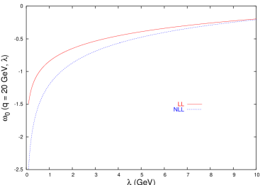
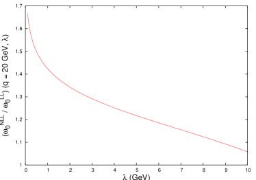
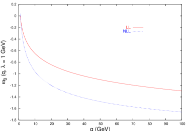
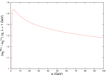
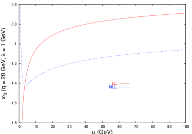
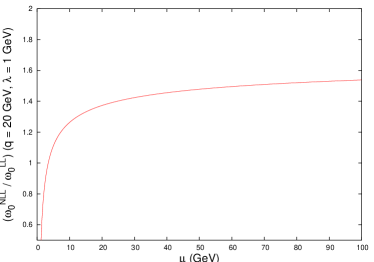
Figure 1: Comparison of the gluon Regge trajectory calculated at LL and at NLL.

For this value of the renormalisation scale the NLL trajectory is always more negative than the LL one with the trajectories separating from each other as the slicing parameter decreases for a fixed $q$, or, when we fix $\lambda$, for large values of $q$. For fixed values of $q$ and $\lambda$, and for large renormalisation scales the effect of changing $\mu$ does not affect the difference between the trajectory at LL and NLL, as can be seen in the bottom two plots in Fig 1. This is not the case for lower values of $\mu$, where the trajectories can even overlap at the minimum of $\omega_{0}^{NLL}$.

To implement the solution for the gluon Green’s function numerically, the kernel in Eq. (6) is rewritten as

$$\widetilde{\mathcal{K}}_{r}\left(q,q^{\prime},\theta\right)~{}=~{}\frac{\bar{\alpha}_{s}^{2}}{4\pi}\left\{\left(1+\frac{n_{f}}{N_{c}^{3}}\right)\left(\frac{3\cos^{2}{\theta}-2}{16}\right)\left(\frac{2}{q^{2}}+\frac{2}{q^{\prime 2}}+\left(\frac{1}{q^{\prime 2}}-\frac{1}{q^{2}}\right)\ln{\frac{q^{2}}{q^{\prime 2}}}\right)\right.$$

$$+\frac{2(q^{2}-{q^{\prime}}^{2})}{\left((q^{2}+{q^{\prime}}^{2})^{2}-4\,q^{2}\,{q^{\prime}}^{2}\,\cos^{2}{\theta}\right)}\left(\frac{1}{2}\ln{\frac{q^{2}}{{q^{\prime}}^{2}}}\ln{\frac{{q}^{2}{q^{\prime}}^{2}\left({q}^{2}+{q^{\prime}}^{2}-2\,q\,q^{\prime}\,\cos{\theta}\right)^{2}}{({q}^{2}+{q^{\prime}}^{2})^{4}}}\right.$$

$$\left.+\left(\int_{0}^{-{q}^{2}/{q^{\prime}}^{2}}-\int_{0}^{-{q^{\prime}}^{2}/{q}^{2}}\right)dt\frac{\ln(1-t)}{t}\right)-\frac{1}{\left(q^{2}+{q^{\prime}}^{2}-2\,q\,q^{\prime}\,\cos{\theta}\right)}\ln^{2}{\frac{q^{2}}{{q^{\prime}}^{2}}}$$

$$-\left(3+\left(1+\frac{n_{f}}{N^{3}_{c}}\right)\left(1-\frac{({q}^{2}+{q^{\prime}}^{2})^{2}}{8{q}^{2}{q^{\prime}}^{2}}-\frac{(2{q}^{2}{q^{\prime}}^{2}-3{q}^{4}-3{q^{\prime}}^{4})}{16{q}^{2}{q^{\prime}}^{2}}\cos^{2}{\theta}\right)\right)$$

$$\hskip 113.81102pt\times\frac{1}{q\,q^{\prime}}\left(\ln{\frac{q^{2}}{{q^{\prime}}^{2}}}\arctan{\frac{q^{\prime}}{q}}+2\,{\rm Im}\left\{{\rm Li}_{2}\left(i\,\frac{q^{\prime}}{q}\right)\right\}\right)$$

$$\left.-\frac{2\,q\,{q^{\prime}}\,\left|\sin{\theta}\right|}{\left(q^{2}-{q^{\prime}}^{2}\right)^{2}+4\,q^{2}\,{q^{\prime}}^{2}\,\sin^{2}{\theta}}\left(\mathcal{F}\left(q,q^{\prime},\theta\right)+\mathcal{F}\left(q^{\prime},q,\theta\right)\right)\right\},$$ (10)

where $\theta$ is the angle between the two–dimensional vectors ${\bf q}$ and ${\bf q}^{\prime}$, and

$$\mathcal{F}\left(q,q^{\prime},\theta\right)~{}=~{}{\rm Im}\left\{4\,{\rm Li}_{2}\left(\frac{q}{q^{\prime}}\,e^{-i\left|\theta\right|}\right)-\ln{\frac{q^{2}}{{q^{\prime}}^{2}}}\ln{\frac{q^{\prime}\,\left|\sin{\theta}\right|-i\left(q-q^{\prime}\,\cos{\theta}\right)}{q^{\prime}\,\left|\sin{\theta}\right|+i\left(q-q^{\prime}\,\cos{\theta}\right)}}\right\}$$ (11)

with

$${\rm Li}_{2}\left(z\right) = -\int^{z}_{0}dt\frac{\ln(1-t)}{t}.$$ (12)

This kernel has an integrable singularity in the ${\bf q}\rightarrow{\bf q}^{\prime}$ limit. As an example of its structure in the vicinity of this singularity we plot $\widetilde{\mathcal{K}}_{r}\left(q,q^{\prime}=20~{}{\rm GeV},\theta\right)$ in Fig. 2 with the same values for the parameters as those in Fig. 1 where the renormalisation scale was fixed to $\mu=30$ GeV.

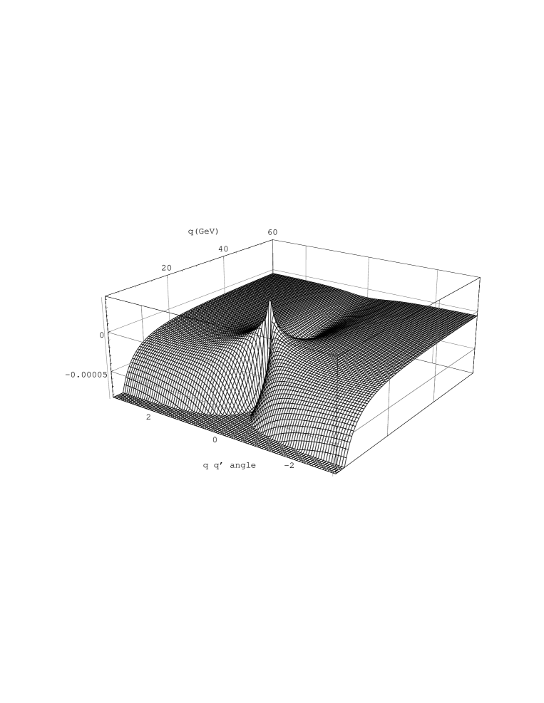
Figure 2: Structure of the kernel $\tilde{K}_{r}\left(q,q^{\prime},\theta\right)$ (in GeV^-2) for $q^{\prime}=20$ GeV as a function of $q$ and the angle between ${\bf q}$ and ${\bf q^{\prime}}$.

In the next Section we use this form of the kernel in order to study the solution to the NLL BFKL equation.

4 Study of the Gluon’s Green Function

We have implemented Eq. (2) in a Monte Carlo integration routine using the form of the kernel presented in Section 3. In the following analysis, we have chosen to run the coupling at one loop, matching the values of Ref. [11] and, as previously explained, we use $\mu=k_{b}$ as the renormalisation scale and set $n_{f}=4$. The function $\xi$ will always correspond to Eq. (7).

4.1 Convergence of the Solution

Before presenting the results for the gluon Green’s function, we first investigate the properties of convergence for Eq. (2). There are two points of interest: Firstly, how the $\lambda\to 0$ limit is approached, and secondly, to determine how many terms in the infinite sum of Eq. (2) are needed to obtain the solution within a given numerical accuracy. These two points are linked because the smaller the value of $\lambda$, the more terms are necessary in the expansion to reach good accuracy, but also the better the approximation $f_{\omega}\left({\bf k}_{a}+{\bf k},{\bf k}_{b}\right)\simeq f_{\omega}\left({\bf k}_{a},{\bf k}_{b}\right)$ for $\left|{\bf k}\right|<\lambda$ (as shown in Ref. [6] this approximation is used in order to write the BFKL equation as in Eq. (2)). A good choice for $\lambda$ is therefore characterised by being small enough for the approximation to be valid, ensuring in this way an accurate answer, while being large enough to warrant the contribution from only a finite number of terms in the expansion, so that the numerical evaluation is fast.

In Fig. 3 we plot the contribution from successive terms in the infinite sum of Eq. (2) to the angular integrated NLL gluon Green’s function

$${\bar{f}}\left(k_{a},k_{b},\Delta\right) = \int_{0}^{2\pi}d\theta\,f\left(k_{a},k_{b},\theta,\Delta\right),$$ (13)

with $\theta$ being the angle between $\mathbf{k}_{a}$ and $\mathbf{k}_{b}$, at ${k}_{a}=25$ GeV, ${k}_{b}=30$ GeV, $\lambda=1$ GeV, and for different values of the parameter $\Delta$. These values have been chosen with no other intention but to illustrate the capability of the NLL formalism proposed in Ref. [6] and its numerical implementation. We see that for a given choice of parameters, only a finite number of terms contribute to the infinite sum. All the results presented in this paper have been calculated with some upper limit on the number of terms included in the infinite sum of Eq. (2). It has been verified that this limit is put sufficiently high as to reproduce the solution with the required accuracy. This plot contains information about how the emission builds up, revealing in a quantitative way the fact that when the energy available for the scattering process is larger, the distribution peaks at larger values of the number of iterations. Although this trend is independent of $\lambda$, the specific position of the peak is not.

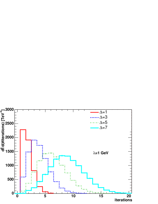
Figure 3: Distribution on the number of iterations in building up the NLL gluon Green’s function for different values of the parameter $\Delta$, at a fixed value of $\lambda=1$ GeV. The gluon Green’s function is evaluated for $k_{a}=25$ GeV, $k_{b}=30$ GeV and the renormalisation scale is chosen to be $\mu=k_{b}$.

$\bar{f}({k}_{a},{k}_{b},\Delta)$ in Eq. (13) could also have been obtained by first angular averaging the BFKL kernel and then solving the equation. Although in our solution we have all the angular information, in this case we average in angles in order to compare with the analytic expression for the LL BFKL gluon Green’s function with zero conformal spin, i.e.

$$\bar{f}\left({k}_{a},{k}_{b},\Delta\right) = \frac{4}{k_{a}k_{b}}\int_{0}^{\infty}d\nu\left(\frac{k_{a}^{2}}{k_{b}^{2}}\right)^{i\nu}e^{{\bar{\alpha}}_{s}\Delta{\chi_{0}}(\nu)}$$ (14)

with the LL eigenvalue being

$$\chi_{0}(\nu) = -2\,{\rm Re}\left\{\psi\left(\frac{1}{2}+i\nu\right)-\psi(1)\right\}.$$ (15)

The LL limit of Eq. (2) is given by

$$f({\bf k}_{a},{\bf k}_{b},\Delta) = \left(\frac{\lambda^{2}}{k_{a}^{2}}\right)^{\bar{\alpha}_{s}\,\Delta}\left\{\frac{}{}\delta^{(2)}({\bf k}_{a}-{\bf k}_{b})+\sum_{n=1}^{\infty}\prod_{i=1}^{n}\bar{\alpha}_{s}\int d^{2}{\bf k}_{i}\frac{\theta\left({\bf k}_{i}^{2}-\lambda^{2}\right)}{\pi{\bf k}_{i}^{2}}\right.$$

$$\times \left.\int_{0}^{y_{i-1}}dy_{i}\left(\frac{\left({\bf k}_{a}+\sum_{l=1}^{i-1}{\bf k}_{l}\right)^{2}}{\left({\bf k}_{a}+\sum_{l=1}^{i}{\bf k}_{l}\right)^{2}}\right)^{\bar{\alpha}_{s}\,y_{i}}\delta^{(2)}\left(\sum_{l=1}^{n}{\bf k}_{l}+{\bf k}_{a}-{\bf k}_{b}\right)\right\}.$$

In this study we have checked that the LL analytic results from Eq. (14) coincide with those from the LL version of our numerical implementation. This will be illustrated in the plots below.

Having shown how it can be checked that a sufficient number of iterations in Eq. (2) has been performed for a given choice of the parameters, we will now proceed to study the $\lambda\to 0$ limit of the equation. In Fig. 4 we have plotted the $\lambda$–dependence of the angular integrated gluon Green’s function on $\lambda$ for a choice of $k_{a}=25$ GeV, $k_{b}=30$ GeV and $\Delta=3$. The result is very flat in $\lambda$ for small values of this parameter, demonstrating, remarkably, the cancellation between the infrared divergences present in the gluon NLL Regge trajectory and those stemming from the integration of the real NLL emission kernel over phase space. For larger values of $\lambda$ we observe a growing $\lambda$–dependence originating from our initial approximation $f_{\omega}\left({\bf k}_{a}+{\bf k},{\bf k}_{b}\right)\simeq f_{\omega}\left({\bf k}_{a},{\bf k}_{b}\right)$ for $\left|{\bf k}\right|<\lambda$. In all the results presented in this work we have taken $\lambda=1$ GeV and checked that this choice is in a region with a very weak dependence on $\lambda$.

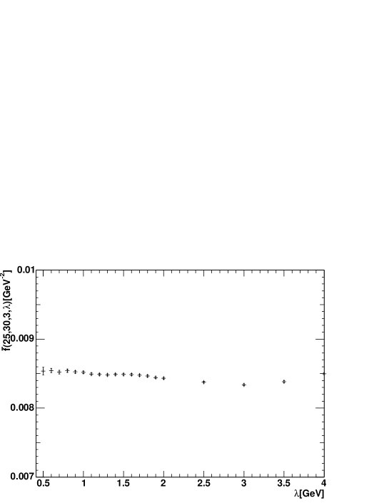
Figure 4: Dependence of the NLL solution for the gluon Green’s function on the parameter $\lambda$ for $k_{a}=25$ GeV, $k_{b}=30$ GeV and $\Delta=3$.

4.2 Dependence of the Gluon Green’s Function on the External Momenta

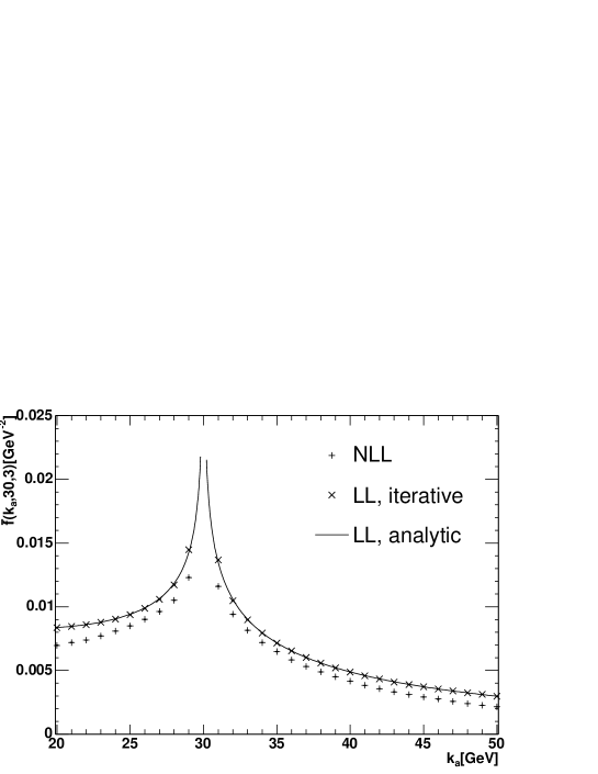
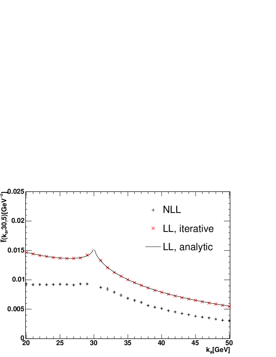
Figure 5: $k_{a}$ dependence of the LL and NLL gluon Green’s function at $\mu=k_{b}=30$ GeV for two values of $\Delta$.

After describing the technicalities of our method of solution we are now ready to show the behaviour of the NLL gluon Green’s function. In Fig. 5 we have calculated $\bar{f}(k_{a},k_{b},\Delta)$ fixing $k_{b}$ at 30 GeV and varying $k_{a}$ for the choice of parameter $\Delta=3$ and $\Delta=5$. We start by noting the complete agreement between the iterative and analytic results at LL. It is also interesting to notice how the angular integrated NLL gluon Green’s function evolves from being strongly peaked in the region $k_{a}\simeq k_{b}$ for small values of $\Delta$ to being more flat in $k_{a}$ for larger values. This behaviour is to be expected, since the BFKL equation can be reformulated as a differential equation in $\Delta$, with $\delta^{(2)}\left({\bf k}_{a}-{\bf k}_{b}\right)$ as the boundary condition at $\Delta=0$. In agreement with this statement we obtain from Eq. (2) that $f\left({\bf k}_{a},{\bf k}_{b},\Delta=0\right)=\delta^{(2)}\left({\bf k}_{a}-{\bf k}_{b}\right)$. By comparing the plots in Fig. 5 we also see how the gluon Green’s function evolves from the boundary condition as $\Delta$ increases.

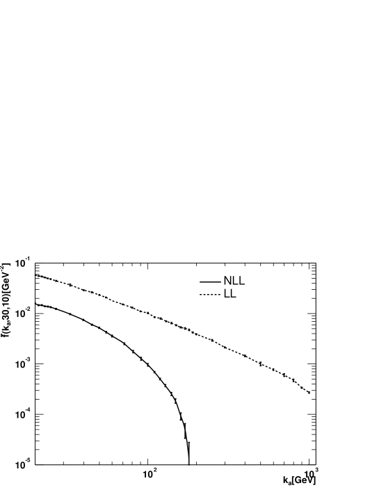
Figure 6: $k_{a}$ dependence of the LL and NLL gluon Green’s function at $\mu=k_{b}=30$ GeV for $\Delta=10$ and a large range in the $k_{a}/k_{b}$ ratio.

Although the normalisation of the gluon Green’s function is different between the LL and NLL cases, and indeed changes with $\Delta$, the shape with respect to $k_{a}$ does not change too much in the $k_{a}\simeq k_{b}$ region. This behaviour is different when $k_{a}\gg k_{b}$, as can be seen in Fig. 6. In this region the gluon Green’s function is much suppressed at NLL compared to the LL case. Similar results were obtained in Ref. [5] when the solution to the BFKL equation was studied using the Mellin transform of the angular averaged kernel, and a similar treatment of the running coupling terms as in our function $\xi$ was considered, i.e. the $\beta_{0}$ terms not resummed into $\alpha_{s}$. In Ref. [5] it was also shown that the resummation of these $\beta_{0}$ terms improves the behaviour of the gluon Green’s function. We will come back to this point in a forthcoming publication.

In principle, it would be interesting to establish whether the Green’s function, as obtained in the present approach, exhibits the exponentially suppressed, oscillatory behaviour predicted in Ref. [3]. For the accessible range of rapidities in our present numerical study it was not possible to verify this effect which would take place at large values of the $k_{a}/k_{b}$ ratio and $\Delta$.

We now proceed to the study of the dependence on $\Delta$ in the next Section.

4.3 Dependence of the Gluon Green’s Function on $\Delta$

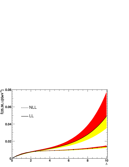
Figure 7: $\Delta$–dependence of the NLL gluon Green’s function evaluated for $k_{a}=25$ GeV and $k_{b}=30$ GeV. The central lines for both the LL and NLL result are obtained by choosing the renormalisation scale $\mu=k_{b}$. The limits of the two upper (red) bands correspond to a choice of renormalisation scale $\mu=k_{b}/2$, while for the bound of the two lower (yellow) bands, the renormalisation scale is $\mu=2k_{b}$.

In Fig. 7 we have plotted the evolution of $\bar{f}(\mathbf{k}_{a},\mathbf{k}_{b},\Delta)$ with $\Delta$ for a specific choice of $k_{a}$ and $k_{b}$, both for the LL and NLL case. We see that for this choice of momenta, there is a significant difference in the $\Delta$–dependence from about $\Delta=3$. With our choice of renormalisation scale of $\mu=k_{b}$, the gluon Green’s function rises slower with $\Delta$ at NLL than at LL. For the range in $\Delta$ studied in this paper no inestability in the growth of the gluon Green’s function has been found. It is known from previous investigations in the literature [5] that a correct resummation of the $\beta_{0}$ terms into the running of the coupling eliminates this possible problem. We will investigate this further in the future.

We study a renormalisation scale dependence by, in Fig. 7, including the results for the choices $\mu=k_{b}/2$ and $\mu=2k_{b}$. At LL, where the coupling does not run, we can still estimate a similar dependence to that at NLL by simply choosing the fixed value of the coupling at LL to be $\alpha_{s}(\mu=k_{b})$, $\alpha_{s}(\mu=k_{b}/2)$ and $\alpha_{s}(\mu=2k_{b})$. This generates the band around the LL result in Fig. 7. The upper (red) bands are obtained for $\mu<k_{b}$, while the lower (yellow) bands correspond to $\mu>k_{b}$. This renormalisation scale dependence is very big at LL and growing with $\Delta$. For the particular selection of parameters, the scale uncertainty is drastically reduced at NLL, with a slow growth with $\Delta$. This last feature has its origin in that as $\Delta$ increases, more powers of $\alpha_{s}$ are effectively resummed because there is more phase space available for emission, as was seen in Fig. 3. The reduction in the uncertainty at NLL with respect to the LL result shows how the predictive power of the theory has improved with the inclusion of radiative corrections. We will study this renormalisation scale dependence in a toy cross–section below, which will include an integration over a range of momenta. But before this, we first analyse in the next Section the angular behaviour of the gluon Green’s function.

4.4 Angular Dependence of the Gluon Green’s Function

One of the advantages of our method of solution is that we can perform studies of angular correlations in the NLL BFKL gluon Green’s function. For example, in Fig. 8 we show the dependence of $f({k}_{a},{k}_{b},\theta,\Delta)$ defined in Eq. (13) for $k_{a}=25$ GeV and $k_{b}=30$ GeV, and the two values $\Delta=3$ and $\Delta=5$. Again we see that for smaller $\Delta$, the transverse momenta $\mathbf{k}_{a}$ and $\mathbf{k}_{b}$ are strongly correlated, with the bulk of the contributions to the gluon Green’s function coming from the region of small angles between the transverse momenta $\mathbf{k}_{a},\mathbf{k}_{b}$. We have included an investigation of the angular correlations of a toy cross section in Section 4.5.

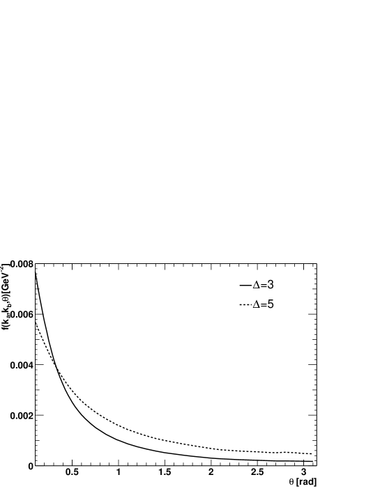
Figure 8: The dependence of the gluon Green’s function at NLL on the angle between $\mathbf{k}_{a}$ ($k_{a}=25$ GeV) and $\mathbf{k}_{b}$ ($k_{b}=30$ GeV) for the choice of $\Delta=3$ and $\Delta=5$. The renormalisation point is chosen at $\mu=k_{b}$.

4.5 Toy Cross Section

We now proceed to the study of the following quantity:

$$S(\Delta)=\int_{k_{a}>30\mathrm{GeV}}\frac{d^{2}{\bf k}_{a}}{{\bf k}_{a}^{2}}\int_{k_{b}>30\mathrm{GeV}}\frac{d^{2}{\bf k}_{b}}{{\bf k}_{b}^{2}}f\left({\bf k}_{a},{\bf k}_{b},\Delta\right),$$ (17)

which, when the gluon Green’s function is evaluated at LL, is proportional to the cross section at this accuracy. We therefore call it a “toy” cross section. A more complete study would require the use of the full NLL impact factors for different physical processes, a calculation which is out of the scope of this paper. Although the accuracy of the impact factors, LL, does not match that of the gluon Green’s function, NLL, the behaviour of $S(\Delta)$ in Eq. (17) with $\Delta$ will still give an indication of the intercept we can expect at NLL.

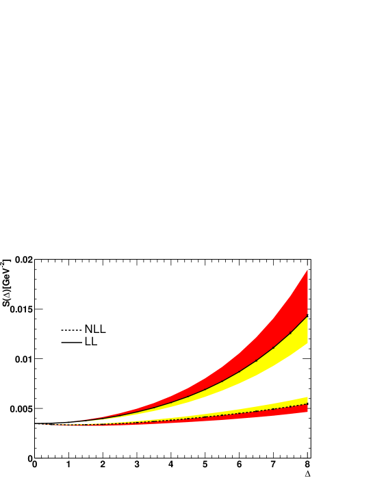
Figure 9: $S(\Delta)$ calculated at LL and NLL, including the renormalisation scale dependence as detailed in the text.

The evolution of the toy cross section with $\Delta$ is shown in Fig. 9 both for the LL and the NLL case. This plot is consistent with the fact that the NLL corrections decrease the intercept of cross sections. With the intention to estimate the renormalisation scale dependence in the LL curve, instead of keeping the strong coupling fixed at, for example its value at the lower integration limits $\alpha_{s}(\mu=30\,{\rm GeV})\simeq 0.14$, we fix it at $\alpha_{s}(\mu=k_{b})$ as we do in the NLL calculation and in our study of the gluon Green’s function in Sections 4.2– 4.4. Again we see, as in Fig. 7, that the renormalisation scale uncertainty is reduced when going from the LL to the NLL curve for our particular choice of $\mu$. When the renormalisation scale is chosen to be larger, the effective value of the coupling is reduced and the LL rise decreases, while the size of the NLL corrections, suppressed by one power of $\alpha_{s}$, diminishes. The overall effect is that the difference between the LL and NLL curves is now smaller than for a lower choice of renormalisation scale. The initial decrease in $S(\Delta)$ in going beyond the LL approximation was already predicted in models adding running coupling effects to the LL evolution [8].

Finally, and in order to illustrate the feasibility of our calculations, in Fig. 10 we have plotted the average value of $\cos(\theta)$, with $\theta$ being the angle between $\mathbf{k}_{a}$ and $\mathbf{k}_{b}$, for the toy cross section as a function of $\Delta$. We see that as $\Delta$ increases, $\mathbf{k}_{a}$ and $\mathbf{k}_{b}$ become increasingly decorrelated, and we see that the effect is bigger at LL than at NLL.

Figure 10: Average value of $\cos(\theta)$ for $S(\Delta)$ at LL and NLL as a function of $\Delta$. At $\Delta=0$ the two transverse vectors $\mathbf{k}_{a}$, $\mathbf{k}_{b}$ are completely correlated, whereas the BFKL evolution leads to a growing decorrelation with $\Delta$, both at LL and NLL. This decorrelation is less at NLL than at LL.

5 Conclusions

In this study we have presented a first analysis of the behaviour of the NLL gluon Green’s function as obtained from a numerical implementation of the method proposed in Ref. [6]. With the main purpose of showing the feasibility of our method we have taken a particular choice of renormalisation scale in the ${\overline{\rm MS}}$ renormalisation scheme. Other choices and schemes can be considered, and work is in progress to study them. We have shown that the convergence properties are well understood, and in particular we have demonstrated the infrared finiteness of our solution. We have also presented results on the evolution and angular dependence of the gluon Green’s function and a toy cross section. The intercept obtained from this procedure decreases at NLL with respect to the one obtained at LL, a trend which is in agreement with results in the literature [4]. The magnitude of the change when going from LL to NLL depends on the choice of renormalisation scale and further studies are needed to draw stronger conclusions.

Acknowledgements We would like to thank Victor Fadin, Stefan Gieseke, Gregory Korchemsky and Lev Lipatov for very useful discussions, the CERN Theory Division for hospitality, and the IPPP, University of Durham, for use of computer resources. A.S.V. thanks the II. Institut für Theoretische Physik at the University of Hamburg and the Laboratoire de Physique Théorique at Université Paris XI for hospitality, and acknowledges the support of PPARC (Postdoctoral Fellowship: PPA/P/S/1999/00446).

References

-
[1]
L. N. Lipatov,
Sov. J. Nucl. Phys. 23 (1976) 338
[Yad. Fiz. 23 (1976) 642],
E. A. Kuraev, L. N. Lipatov and V. S. Fadin, Sov. Phys. JETP 45 (1977) 199 [Zh. Eksp. Teor. Fiz. 72 (1977) 377],
I. I. Balitsky and L. N. Lipatov, Sov. J. Nucl. Phys. 28 (1978) 822 [Yad. Fiz. 28 (1978) 1597]. -
[2]
L.N. Lipatov, JETP , 904 (1986),
G. Camici and M. Ciafaloni, Phys. Lett. B , 118 (1997),
R. S. Thorne, Phys. Lett. B 474 (2000) 372,
J. R. Forshaw, D. A. Ross and A. Sabio Vera, Phys. Lett. B 498 (2001) 149,
R. S. Thorne, Phys. Rev. D 64 (2001) 074005,
M. Ciafaloni, M. Taiuti and A. H. Mueller, Nucl. Phys. B 616 (2001) 349,
M. Ciafaloni, D. Colferai, G. P. Salam and A. M. Stasto, Phys. Lett. B 541 (2002) 314,
M. Ciafaloni, D. Colferai, G. P. Salam and A. M. Stasto, Phys. Rev. D 66 (2002) 054014. - [3] D.A. Ross, Phys. Lett. B431 (1998) 161.
-
[4]
Yu.V. Kovchegov and A.H. Mueller, Phys. Lett. B439 (1998)
423,
J. Blümlein, V. Ravindran, W.L. van Neerven and A. Vogt, preprint DESY-98-036, hep-ph/9806368,
E.M. Levin, preprint TAUP 2501-98, hep-ph/9806228,
N. Armesto, J. Bartels, M.A. Braun, Phys. Lett. B442 (1998) 459,
G.P. Salam, JHEP 8907 (1998) 19,
M. Ciafaloni and D. Colferai, Phys. Lett. B452 (1999) 372,
M. Ciafaloni, D. Colferai and G.P. Salam, Phys. Rev. D60 (1999) 114036,
R.S. Thorne, Phys. Rev. D60 (1999) 054031,
S. J. Brodsky, V. S. Fadin, V. T. Kim, L. N. Lipatov and G. B. Pivovarov, JETP Lett. 70 (1999) 155,
C. R. Schmidt, Phys. Rev. D 60 (1999) 074003,
J. R. Forshaw, D. A. Ross and A. Sabio Vera, Phys. Lett. B 455 (1999) 273,
G. Altarelli, R. D. Ball and S. Forte, Nucl. Phys. B 575 (2000) 313,
G. Altarelli, R. D. Ball and S. Forte, hep-ph/0306156. - [5] M. Ciafaloni, D. Colferai, G. P. Salam and A. M. Stasto, hep-ph/0307188.
- [6] J. R. Andersen and A. Sabio Vera, Phys. Lett. B 567 (2003) 116.
-
[7]
J. Kwiecinski, C. A. Lewis and A. D. Martin,
Phys. Rev. D 54 (1996) 6664,
C. R. Schmidt, Phys. Rev. Lett. 78 (1997) 4531,
L. H. Orr and W. J. Stirling, Phys. Rev. D 56 (1997) 5875. -
[8]
W. J. Stirling,
Nucl. Phys. B 423 (1994) 56,
L. H. Orr and W. J. Stirling, Phys. Lett. B 429 (1998) 135,
L. H. Orr and W. J. Stirling, Phys. Lett. B 436 (1998) 372,
J. R. Andersen, V. Del Duca, S. Frixione, C. R. Schmidt and W. J. Stirling, JHEP 0102 (2001) 007,
J. R. Andersen, V. Del Duca, F. Maltoni and W. J. Stirling, JHEP 0105 (2001) 048,
J. R. Andersen, Acta Phys. Polon. B 33 (2002) 3001,
J. R. Andersen et al., J. Phys. G 28 (2002) 2509,
J. R. Andersen and W. J. Stirling, JHEP 0302 (2003) 018. - [9] V. S. Fadin and L. N. Lipatov, Phys. Lett. B 429 (1998) 127.
- [10] M. Ciafaloni and G. Camici, Phys. Lett. B 430 (1998) 349.
- [11] A. D. Martin, R. G. Roberts, W. J. Stirling and R. S. Thorne, Eur. Phys. J. C 14 (2000) 133.